Uncertain Operating Conditions Implications on Multistage Operations Optimal Design and Environmental Impact

Abstract

Energy demand is increasingly the most relevant cost item in chemical plants. Operating expenses indeed play a main role in all plants processing large amounts of feedstock via well-established processes in the petrochemical industry. In staged operations, the optimal number of stages is usually obtained by means of an economic optimization. However, the designed equipment, external duties, and thus operating expenses may considerably vary under the effect of external disturbances. The main purpose of this paper is to outline a simple but effective procedure to account for perturbations in the assessment of the optimal number of stages. The analysis shows that appropriate investments could lead to a unit design able to mitigate the higher duty requirements when external perturbations occur. The results highlight that the optimal number of stages varies when uncertainty is considered and, with low computational effort, this can be effectively quantified by means of the applied methodology. Furthermore, the same approach has been applied to sustainability indicators over the uncertain domain as well. In those cases, when more stages correspond to more flexible equipment, the environmental impact is positively affected, and a double benefit can be observed.

1. Introduction

Multistage separations (especially distillation) are widespread operations present in the vast majority of chemical plants. They play a main role both on process and on utility sides, consuming large amounts of energy in the form of heat and electricity. Common examples are crude oil topping (distillation in general), multistage non-adiabatic reactors, steam generation, and drying operations, as well as concentration processes such as multiple-effect evaporation [1]. The most basic procedure for equipment design and sizing refers to nominal operating conditions, and the remaining degrees of freedom are fulfilled by means of an economic optimization. In particular, for multistage units, the optimal number of stages can be detected according to the Total Annualized Costs (TAC) able to synthesize the impact of Capital and Operating Expenses (CAPEX and OPEX, respectively) as well as depreciation over time [2].

Therefore, for a given equipment configuration, the control system is the part aimed at mitigating the influence of external disturbances [3] by managing the external duties according to the specifications, i.e., OPEX are the main cost item related to external disturbance suppression. In particular, the external duties oscillation magnitude is strictly related to the number of separation stages. The mitigation of duty fluctuations also provide benefits from a safety, operational, and environmental point of view. The energy consumption, in particular the electricity for compression and heat duties [4,5,6], is indeed the main item in the list of factors affecting the environmental impact of a process. Therefore, a more proper system design able to effectively cope with external perturbations could not only result in a higher profitability but also in lower emissions.

Design under uncertainty has been extensively discussed during the last decades. At first, the proposed methodologies were based on stochastic design problem solutions with two- or multiple-stage approaches [7]. Dedicated mathematical programming techniques [8,9] as well as the inclusion of planning [10] or operations research problems [11] have been analyzed. Other approaches have been suggested involving the use of probabilistic constraints [12], genetic [13,14] and sampling averaging algorithms [15], Bayesian model averaging [16], and, in order to reduce the computational effort, scenario-free approaches have been proposed as well [17,18,19]. In process systems, when dealing with uncertainty the concept of flexibility arises. A flexible design is defined as a design able to ensure feasible operation over a given range of uncertain parameter deviation [20]. Both deterministic [21,22] and stochastic [23,24] flexibility indicators have been proposed in the literature over the last few decades. In this perspective, flexibility analysis can be seen as a worst-case analysis to identify the most constraining parameters from a feasibility point of view [25].

Concerning the analysis of energy systems consumption accounting for uncertainty, recent works are available in literature as well. In these cases, the uncertainty is related to energy source availability [26], system failure [27], and economic aspects [28,29], and they all address the CO₂ emissions assessment.

In the light of these premises, this study was conducted in order to account for uncertainty with a specific focus on the problem of the optimal number of stages in multistage unit operations and the related energy consumption. In particular, with respect to the available literature, here the main purpose is to suggest an approach based on the uncertainty characterization that implies the reformulation of the operating expenses. The main advantage of this methodology is its quick application and low computational effort with respect to other, more complete tools (e.g., multi-level stochastic optimization). Different from other literature works, this article addresses the specific unit operations design, and the number of stages is the design parameter of interest that is adjusted to compensate the impact of upstream perturbations on the utility consumption. By analogy, it is the reference parameter for the environmental impact assessment that is included among the decisional criteria. Finally, the main limitation of this approach is that its lower computational effort can be exploited only given that the deviation probability distribution function is known.

The mathematical details of the uncertainty characterization and of the proposed methodology are explained in detail in the next section.

2. Methodology

This section is made of three parts and presents the main features of the design approach proposed in this research work. The first part concerns the uncertainty characterization and briefly introduces its classification as well as the reasons why its impact on the optimal unit operations design could be worth a dedicated study. On the other hand, the design procedure under nominal operating conditions and the one accounting for process parameters deviation are discussed in detail in the second part. In particular, this subsection provides an explanation of the items contained in the cost function to minimize and focuses on how the uncertainty characterization can be included in the methodology used to assess the optimal unit design. Finally, in the third part, the main premises and hypotheses concerning the environmental impact assessment are discussed to give the basis for the related results understanding.

2.1. The Uncertainty Characterization

Although the purpose of this study is to outline a thorough procedure of general validity, the results obtained are nevertheless qualitatively and quantitatively case specific. In particular, one of the aspects with the highest impact on the results is the distribution function (hereafter PDF) selected to describe the uncertain variables’ fluctuation probability.

Uncertainty indeed has been one of the key aspects related to design optimization methodologies during the past years. The different typologies of uncertainty have been classified by Oberkampf and Helton (2012) [30] into three main categories:

• Aleatory uncertainty (also referred to as stochastic uncertainty, irreducible uncertainty, inherent uncertainty or variability);
• Epistemic uncertainty (also referred to as reducible uncertainty, subjective uncertainty, model form uncertainty or simply uncertainty);
• Error.

This is the reference classification still used nowadays by the vast majority of authors dealing with uncertainty in different domains [31]. Aleatory uncertainty is defined as the inherent variation associated with the physical environment under consideration, while the epistemic uncertainty is defined as any lack of knowledge or information in any phase or activity of the modeling process. Error is defined as a recognizable deficiency in any phase or activity of modeling and simulation that is not due to lack of knowledge [30,32,33]. Epistemic uncertainty has been one of the most challenging topics during the past years and it can be concluded that its characterization is better carried out by means of fuzzy sets theory [34], Dempster-Shafer theory [35], possibility theory [36], and the theory of upper and lower previsions [37]. Several studies discussing computational methods for optimization accounting for this kind of uncertainty are available in literature for more details [12,38,39,40].

On the other hand, aleatory uncertainty is particularly suitable for input data variability descriptions, and it is widely agreed that it can be characterized by using the probability theory, i.e., by means of probability distribution functions [30,31,41,42]. This kind of design under stochastic uncertainty is typically referred to as flexibility-based design, as thoroughly discussed by several research works available in the literature [20,21,22,23,24,43,44,45,46,47].

Disturbance probability can be described both by discrete and continuous PDFs based on data collection and measurements related to the process or as the product of reasonable assumptions about the perturbation nature and magnitude. In this research work, the normal (Gaussian) and the Gamma probability distributions, represented in Figure 1a,b with their cumulative functions, have been used in order to describe two different and common process variables behaviors (for further details about the mathematical formulation of the mentioned PDFs, please refer to Severini (2011) [48]) and to provide quantitative outcomes.

This work indeed focuses on the effect of uncertainty on process design, and these two distributions are particularly useful to represent two main categories of events, as further detailed here below, and to emphasize the impact on the final results. In fact, whenever no information is available, a general validity PDF should be employed, and the normal distribution is the one usually describing this “general validity” condition. Moreover, uncertainty is often due not only to the uncertain variable fluctuation, but to the error related to its measurements. Once again, the Gaussian PDF appears to be the most suitable distribution to describe this phenomenon.

When shifting from the deterministic to the stochastic domain, the nominal operating conditions are often identified as the most probable operating conditions. The symmetry of the normal PDF implies that negative deviations with respect to the nominal operating conditions are as probable as positive ones with the same magnitude. However, in chemical processes, this is not always the case since external perturbations often preferentially occur in one particular direction. For this reason, the Gamma PDF is included in the analysis as well. This particular PDF was considered a suitable choice to describe very common situations where the nominal value represents the most probable condition, but it actually underestimates the vast majority of the possible operating conditions. If the cumulative probability is considered in correspondence with the operating point, i.e., the maximum probability, less than the 20% of all possible operating conditions are actually included. From a process design point of view, this means that if the equipment sizing is performed with respect to nominal operating conditions, the obtained design is undersized for more than the 80% of the plant operation.

For the sake of completeness, it is worth clarifying that in this research work, since the Gamma PDF decreasing trend shows a very low slope for very high x values, it was truncated at 98% of its cumulative distribution function to fit the incertitude interval without affecting the obtained results, as shown in Figure 1b.

Therefore, in order to couple uncertainty and optimal design procedure, a reliable perturbation range for the x-axis of Figure 1a is defined in detail according to the specific unit under analysis in the corresponding case studies sections.

2.2. Design Procedure

As already mentioned, the methodology proposed in this article to determine the optimal number of stages in multistage unit operations under uncertain operating conditions is an application to those cases whose aleatory uncertainty can be described by means of a probability distribution function. The purpose of this section is to sum up the concepts previously presented and to group them in a procedure that will be used in this research work.

First, the optimal design under nominal operating conditions is performed by minimizing the annualized costs. For the case studies addressed in this research work, capital expenses were calculated according to the Guthrie-Ulrich-Navarrete correlations [49,50,51,52], while operating expenses were assessed according to the actual price of steam per unit energy, both for the evaporator external steam and for the column reboiler duties as later described. The cost estimation correlations for both CAPEX and OPEX according to the selected unit are further detailed in Appendix A.

Finally, the TAC is defined as:

$$TAC \left[\$/y\right]=OPEX+CRF\cdot CAPEX$$

(1)

where the CRF is the Capital Recovery Factor and it is given as:

$$CRF=\frac{i\cdot {\left(1+i\right)}^n}{{\left(1+i\right)}^n-1}$$

(2)

where i is the discount rate and n is the unit lifetime [53]. This coefficient accounts for capital depreciation over time. The most suitable values for those two terms can be found in the available literature and databases according to the specific process unit [54,55].

After that, a second design procedure is performed in order to account for the uncertain operating conditions impact on operating costs. Although the procedure does not depend on the uncertainty PDF, some specific trends should be used in this work to present some quantitative results. It is worth remarking that the uncertain variable probability is a property of the particular system and cannot be selected. It can be obtained from data collection or by means of reliable assumptions based on the process nature.

In this research work, two different PDFs were proposed to characterize the uncertainty, as shown in Figure 1. These two trends were selected in order to compare the impact of both symmetric and skewed disturbance PDF on the final result. The Gamma and the normal PDF belong to the two-parameter distributions family; therefore, two conditions should be fixed in order to uniquely define them. For this study, the first condition is that the nominal operating conditions correspond to the maximum of the PDF curves, i.e., the operating condition most likely to occur. On the other hand, the two distributions were selected so that their variance was the same.

As already pointed out, although the deviation PDF is not an arbitrary choice, these assumptions are just exploited to show the impact of some common behaviors on the final design. Indeed, the normal PDF was used to describe the most common probability distribution, taking into account the measurement errors as well, while the Gamma was included for all those processes whose input varies over a range with asymmetrical behavior.

Then, given the uncertainty characterization, the operating conditions are evaluated over the uncertain domain by weighing each operating condition according to its probability, according to the equation:

$$OPE{X}^{*}=\frac{1}{x^{max}-x^{min} }\cdot {{\displaystyle \int }}_{x^{min}}^{x^{max}}OPEX\left(x\right)\cdot P\left(x\right)\cdot dx$$

(3)

where x refers to a generic operating condition.

The TAC function is then calculated by accounting for both the CAPEX and the newly obtained OPEX trends. Finally, the optimal number of stages is assessed once again as usual. Before applying the procedure to the case studies, some properties of the integral here above can be already pointed out in order to outline some expectations and to acquire a preliminary sensitivity to this probability-based averaging.

Let us consider, for instance, a symmetric PDF and a linear trend of the OPEX function over the considered uncertain domain. Given that a = x^max − μ = μ − x^min, the integral, referring to the PDF mean, becomes:

$$OPE{X}^{*}=OPEX\left(\mu \right)+\frac{1}{2a}\cdot {{\displaystyle \int }}_{-a}^{a}OPEX\left(x-\mu \right)\cdot P\left(x-\mu \right)\cdot dx$$

(4)

Being the term inside the integral, the product between a symmetric (even) and a linear (odd) function is an odd function as well. This means that the outcome of this integral average is exactly the value of the OPEX function at the center of the domain, i.e., the OPEX value calculated under nominal operating conditions.

In brief, for these kinds of systems, it can be known “a priori” that a more detailed design procedure would only result in useless computational effort. On the other hand, in the case of asymmetric distribution, a linear trend of the cost function would result in a non-zero value for the integral in Equation (4) and the function OPEX* would be shifted with respect to OPEX(μ) accordingly. In order to validate this observation, in this research work calculations with the Gaussian PDF were performed even when the cost function trend could be approximated to a linear one.

After the economic assessment, an environmental impact evaluation can be performed in order to check if the different optimal number of separation stages with respect to the nominal operating conditions results in lower or higher emissions. In general, when accounting for uncertainty, the design requires more stages than the conventional one, i.e., lower OPEX and then lower duty demand. In these cases, both economics and sustainability would benefit from the additional stages. Regardless of whether a different outcome was obtained, the environmental footprint should be included among the optimization criteria as a part of a more complex algorithm in order to have an optimal design based both on economic and sustainability aspects. The latter are further explained in the following Section 2.3.

2.3. Environmental Impact

Sustainability is by far a topic of major concern over the last years in the engineering domain. The energy challenge is the key point of the environmentally friendly policies adopted by all of the most developed and industrialized countries worldwide. For this purpose, Horizon 2020, i.e., the biggest EU Research and Innovation program, was funded by the European Union over the 2014–2020 period [56]. On the other hand, the International Energy Agency defines renewables as the center of the transition to a less carbon-intensive and more sustainable energy system [57]. However, since the transition from fossil fuels to renewables requires a considerable time span to establish itself, the short-term solution lies in more energy-effective technologies.

In the light of these premises, during the design phase, besides the economic comparison between operating and capital expenses, particular attention should be dedicated to the former from a sustainability point of view. A lower number of separation stages implies a considerably higher energy demand in the case of external perturbations, even when they result in a more profitable design. Referring to the previous case studies, an overdesign would result in a more profitable and more sustainable operation. In order to quantify the environmental impact as a function of the energy demand of process units, the Global Warming Potential indicator was employed since it was proven to have the most adverse effect on the sustainability profile of the case study operations [58]. The CO₂ emissions were calculated according to the methodology followed by Gadalla et al. (2006) [59] as a direct function of the duty requirement.

Even though CO₂ emissions are strictly correlated to the fuel employed to produce the required energy, this study carried out a comparison between different configurations of the same unit. Therefore, the study can be considered fuel-independent. The results presented in this paper refer to natural gas. For the same reason, CO₂ emissions related to feedstock and products cancel out when computing the difference between two configurations. According to several authors [59,60,61,62], taking into account the plant lifetime, the CO₂ emissions associated with the installation of additional units/stages are negligible with respect to the emissions related to the heat requirement. By analogy, although the CO₂ emissions due to pumping and cold duties were thoroughly calculated using a specific emissions factor of 51.1 kg_CO2/GJ, as suggested by Waheed et al. [6], they resulted in orders of magnitude lower with respect to the steam duty, as already proven by several studies [6,60,61,62].

For more details about the CO₂ emissions calculations, please refer to Appendix B.

The following section shows in detail the two case studies to which the entire procedure described here above were applied.

3. Case Studies

In this section, two multistage unit operation case studies are presented. The design of a multiple-effect evaporator and a standard distillation column were performed in order to assess the optimal number of stages able to minimize the total costs. The same units were then designed, accounting for uncertain operating conditions characterized by means of both symmetric and skewed PDFs to compare the impact of different deviation qualitative behavior.

Evaporation and distillation were selected since they are among the most widely spread operations in chemical plants and, thus, the impact of uncertain operating conditions, even for simple applications, on their optimal configuration is of particular interest. Moreover, the choice of two case studies also shows that uncertainty could considerably affect both concurrent and countercurrent operation designs.

The detailed description of nominal operating conditions, process specifications, and model equations is provided here below for each case study in the corresponding section.

3.1. Multiple-Effect Evaporator

The first case study refers to a concurrent multiple-effect evaporator. It is a non-conventional unit operation made up of several flash units in series (cf Figure 2) and it can be used either to concentrate a solution (sometimes up to crystallization) or to recover a valuable solvent from it. The main advantage of this unit, with respect to the corresponding single effect configuration, is that the outlet vapor of each effect can be used as external duty for the following one which enhances the separation. The cost of this operation improvement consists of the need for an additional unit and also of the pressure drops required in order to reduce the solution boiling temperature below the previous vapor condensation one.

This basic operation was selected as a first example in order to show how, even for a simple and non-sensitive process, taking into account operating conditions fluctuations could lead to small but significant OPEX changes affecting the optimal design choice.

The concurrent multiple-effect evaporator was modeled according to Di Pretoro et al. (2020) [63,64]. For each effect, the model equations state as follows:

• Overall mass balance

$$L_{i-1}=L_i+V_i$$

(5)

where L and V are the liquid and vapor flowrates;

• Component mass balance

$$L_{i-1}\cdot w_{i-1}=L_i\cdot w_i$$

(6)

where w is the solute mass fraction;

• Energy balance

$$L_{i-1}\cdot c_L^P\left(w_{i-1},T_{L,i-1}\right)\cdot T_{L,i-1}+V_{i-1}\cdot \Delta H_{ev}\left(T_{V,i-1}\right)=L_i\cdot c_L^P\left(w_i,T_{L,i}\right)\cdot T_{L,i}+V_i\cdot (c_P^{water}\cdot T_{L,i}+\Delta H_{ev}\left(T_{V,i}\right))$$

(7)

where T_L and T_V are the vapor and liquid temperatures, c_P^L is the liquid specific heat, and ΔH_ev is the evaporation enthalpy;

• Heat exchanger characteristic equation

$$Q_i=V_{i-1}\cdot \Delta H_{ev}\left(T_{V,i-1}\right)=U_i\cdot A_i\cdot \left(T_{V,i-1}-T_{L,i}\right)$$

(8)

where Q is the heat duty, U is the heat transfer coefficient, and A is the heat transfer surface area for the i-th effect;

• Boiling point elevation

$$\Delta T_{eb,i}=T_{L,i}-T_{V,i}=f\left(w_i\right)$$

(9)

It is worth noting that the solute is considered a non-volatile species, i.e., its molar fraction in the vapor phase is equal to zero. Furthermore, correlations for evaporation enthalpy, specific heat, and boiling point elevation are those provided by the Perry’s Chemical Engineers’ Handbook [1].

For reasons related to economic convenience, all the units are equal to each other. As a consequence, every evaporator has the same heat transfer surface area that is large enough to manage the system perturbations.

Each evaporator thus has five degrees of freedom (L, V, w, T_L, T_V), each of which is satisfied by one of the five model equations. The specification xN concerning the last effect fulfills the d.o.f. related to the external steam duty V₀.

Table 1. Nominal operating conditions.

Property	Value	Unit
L0	10,000	kg/h
TL,0	363.15	K
x0	0.05	kg/kg
TV,0	393.15	K
wN	0.5	kg/kg

shows the feed stream properties as well as the external steam duty temperature and the outlet concentration specification for the case study under analysis in this paper. With regards to the uncertain operating conditions characterization required to perform the design according to the proposed procedure, the inlet flowrate was identified as the variable likely to undergo external disturbances. Given that the nominal operating conditions can be identified as the operating point of maximum probability, i.e., the PDF mode, according to the Gaussian and Gamma variance hypothesis described in Section 2.1, the uncertain domain was assumed to vary over the interval (9000, 16,500 kg/h).

3.2. Distillation Column

The second case study refers to a standard binary distillation column unit. In

Table 2. Distillation feed properties and nominal operating conditions.

	Property	Value	Unit
Feed
	F	38	kmol/h
	Tfeed	397.15	K
	zPhenol	0.35	mol/mol
Specifications
	Ptop	1.013	bar
	xDCyclohex	0.95	mol/mol
	xBPhenol	0.80	mol/mol

, the feed properties under nominal operating conditions, the operating pressure, and the distillate and bottom products specifications are listed. Despite the higher complexity of the process under analysis, a simple cyclohexanol/phenol mixture without thermodynamic singularities (such as azeotrope or unusual equilibrium curves) was selected for the separation in order to avoid results strictly related to the particular case study. Moreover, the selection of a common process is more suitable to show the methodology effectiveness even with respect to ordinary applications. The employed thermodynamic equation of state for the equilibrium calculations was the Soave-Redlich-Kwong and the column Murphree efficiency for the assessment of the real number of trays was 0.5.

Even in this case, to carry out the proposed design procedure accounting for disturbances, a proper uncertain interval (0.31, 0.58) was selected for the uncertain variable that was identified as the inlet composition. The aim of this choice was to highlight the sensitivity of the process with respect to an intensive variable instead of the system capacity.

4. Results and Discussion

In this section, the results for the conventional design under nominal operating conditions and the procedure accounting for uncertain variables deviation are compared. They are listed in subsections according to each case study in order to analyze the outcome deriving from an uncertain feed stream flowrate and composition to be treated, respectively.

4.1. Multiple-Effect Evaporator

As already introduced in Section 3.1, an increase in the number of consecutive evaporation stages, i.e., higher CAPEX, reflects in an OPEX decrease. Since the product is always the same given amount of concentrated solution (for this case study L_N = L₀·w₀/w_N = 1000 kg/h), maximizing the net income corresponds to minimizing the Total Annualized Costs (TAC).

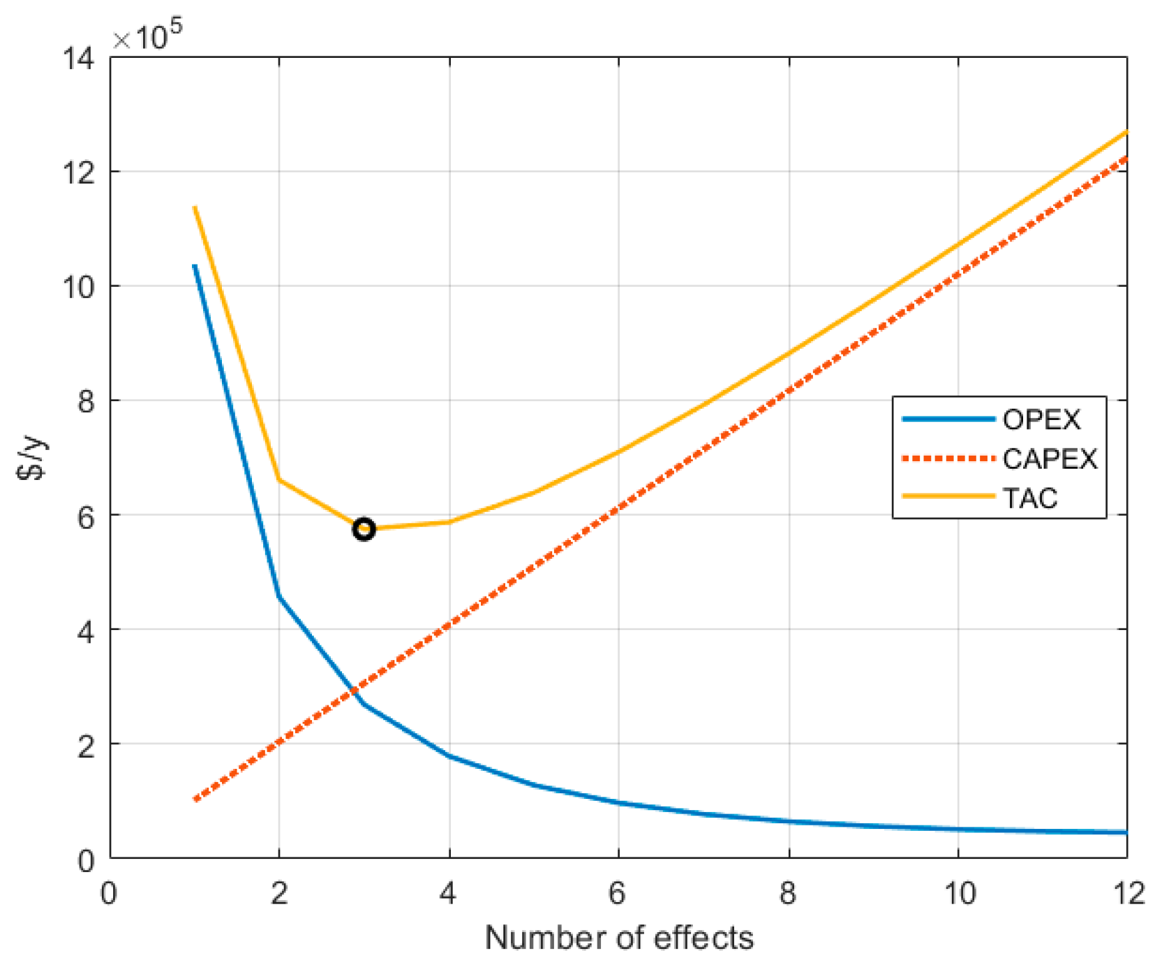
Figure 3 shows the trend of the two curves (in USD/year) as well as the total costs, obtained by the combination of the two, vs the number of effects ranging from 1 up to 12. The OPEX curve, representing the external duty requirement, has a hyperbolic trend while the CAPEX has a linear increase with respect to the number of units employed. The optimal number of effects is three and the corresponding total annualized cost is 574,882 USD/year.

The multiple-effect evaporator model can then be solved for both variable number of stages and over the entire interval of uncertain operating conditions. Figure 4a shows the external energy requirement for each number of effects at each value of the feed flowrate. This external duty represents the energy provided by the condensing steam utility in the first evaporation stage.

As expected, the steam needed to concentrate the solution up to the specification achievement is higher for a lower number of stages and for a higher flowrate to be processed. Moreover, it can be noticed that the duty increase itself is higher for a lower number of effects (cf Figure 4). This means that the feed flowrate perturbation is distributed over the effects, and it becomes almost irrelevant for several effects higher than 10, for which we expect the flexible design to provide a result very similar to the conventional one.

In light of the above, a relevant OPEX curve shift towards higher values can be expected which is higher as N is lower.

The operating costs were then averaged over the uncertain domain according to Equation (3). A new OPEX trend reflecting the uncertainty contribution was then obtained. As it can be noticed in Figure 4b, the external duty can be considered a linear function of the inlet feed flowrate (R² = 0.9974). The results obtained with the use of the normal distribution to describe the uncertain variable deviation give, as expected, the same values as the nominal case in Figure 3 independently from the selected variance due to the function properties already discussed in Section 2.1. Thus, since trends overlap, they cannot be distinguished on the plot.

On the other hand, Figure 5 represents the new TAC plot according to the deviation Gamma PDF. The TAC trend is still calculated according to the Equation (1) where CAPEX is still the same, since it depends on the equipment only, while OPEX are obtained according to the Equation (3).

The results thus obtained, denoted by the dashed lines, reflect the expectations. In general, the total annualized costs were higher than those assessed by considering the nominal operating conditions. The minimum moves to the right due to the higher OPEX increase are related to a low number of effects, while the two curves asymptotically overlap each other for higher values of N. The optimal design under uncertain operating conditions accounts for four evaporation stages with a TAC equal to 651,438 USD/year.

The outcome of the analysis carried out on this first case study might seem trivial. However, given the simplicity of the selected process as well as its relatively low sensitivity with respect to the selected uncertain variable, this example shows how an a priori flexibility analysis can significantly affect the design choice and allows for a more cost-saving decision.

In order to better show the uncertain operating conditions’ impact on the costs and the relevant bias usually neglected while performing a design optimization without considering external disturbances, the results for a more sensitive process are presented in the next section.

4.2. Distillation Column

The distillation column was simulated under nominal operating conditions by means of ProSim Plus^® process simulator in order to assess the condenser and reboiler duties, the reflux ratio, and the maximum and minimum volumetric flowrates flowing along the unit. Given these data, the equipment sizing was performed in order to evaluate the capital expenses for each number of theoretical trays from 9 to 32.

Results are reported in Figure 6. As usual, the operating costs show an asymptotic trend with an increasing number of stages. The reflux ratio indeed approaches the R_min value as a higher number of stages is used. This lower reflux results in lower boilup and condenser duties, which explains the behavior of the OPEX curve.

Capital costs have the standard linear trend as well, except for very low number of trays. This behavior is due to the column diameter as well as reboiler and condenser heat transfer surface area oversizing related to the extremely high reflux ratio attained when getting close to the minimum number of stages (N_min = 7).

The total annualized cost function shows the typical trend with a minimum, and the corresponding optimal number of theoretical equilibrium stages is 16 (reboiler included) with a TAC equal to 224,472 USD/y.

After that, a preliminary sensitivity analysis was performed as usual, and the results are represented in Figure 7. As expected, the obtained surface reflects the typical higher energy demand for a lower number of separation stages; an analogous trend can be detected for the condenser duty even though the cooling water contribution to operating expenses is one order of magnitude lower than the reboiler steam one.

Different from the multiple effect evaporator case study, the heat duty trend with respect to the phenol molar fraction in the feed can be either increasing or decreasing in the considered interval according to the number of equilibrium stages.

This phenomenon can be more easily detected from a lateral perspective, as shown in Figure 7b. For a small number of stages, a higher duty is required if the feed phenol content is higher than the cyclohexanol one. However, for a large number of stages, a higher duty is required if the feed cyclohexanol content is higher than the phenol one. There exists an intermediate condition as well around 14 stages where the feed composition perturbation has a low impact on the duties.

Once again, the OPEX can be averaged over the uncertain variable probability distribution function according to Equation (3).

If the normal PDF is considered, almost the same result as the nominal design is obtained due to the symmetry of the distribution and the almost linear trend of the energy costs with respect to z_Phenol (R² = 0.9912).

On the other hand, the use of an asymmetric probability distribution such as the Gamma PDF to describe the feed composition uncertainty results in a relevant impact. Figure 8 shows the new OPEX curve averaged with respect to the skewed distribution as well as the corresponding TAC function according to the procedure already explained in Section 2.2. The averaged costs for external duties under uncertain conditions are higher than those related to nominal operating conditions in the case of low number of stages and lower for a high N value. This “rotation” of the OPEX curve causes the total costs point of minimum displacement to land at 18 equilibrium stages with a corresponding TAC value equal to 222,992 USD/y.

To conclude the results analysis of the distillation column case study, it can be observed that, different from the multiple-effect case study where the OPEX function was stretched towards higher values for a low number of stages, in this case the OPEX curve rotated, causing the new optimal TAC value to be even lower than the nominal one.

Moreover, the distillation process was particularly sensitive to the feed composition uncertainty. Indeed, two additional stages out of 16 were a non-negligible oversizing requirement; this result was even more appreciable if we take into account that the selected separation process involved an ideal mixture whose components could be easily separated. Finally, in both cases the design based on flexible operating conditions resulted in a higher number of stages able to mitigate duties and additional costs if perturbations were to occur.

5. Environmental Impact Assessment

As an analogy along with Section 4, the results for the environmental impact assessment are presented below for the multiple-effect evaporator and the distillation column case studies, respectively. As already introduced in Section 2.3, the selected indicator is the Global Warming Potential, and its value is assessed for variable number of effects/stages over the uncertain domain. For the nominal case, the reported value corresponds to the nominal duty consumption, while for the flexible design it is the result of the same averaging procedure performed with the OPEX in the economic assessment.

The average values of equivalent CO₂ emissions for the multiple-effect and for the distillation case studies are shown, respectively, in Figure 9a,b.

Both the plots reflect the OPEX function trend, which is the heat duty curve, as expected. For a higher number of stages, the energy demand is lower and thus the equivalent CO₂ emissions are lower, both under nominal and uncertain operating conditions. These results validate the initial remark highlighting the fact that, for these particular case studies, a higher value of N implies both economic and environmental advantages with apparently no drawbacks.

However, in order to have a more reliable interpretation of these results, further study is warranted by using equivalent CO₂ emissions per functional unit, as outlined by the ISO14040 [65], instead of the emissions per operating time. Regarding the functional unit, the two main possible choices are either a kg of treated stream or a kg of purified product. Since those units perform separation processes, it can be assumed that they are designed to treat feedstocks, and thus 1 kg of feed stream can be used as functional unit.

Moreover, for the multiple effect evaporator, both in the case of solvent recovery and solution concentration, the product quantity is proportional to the feed flowrate due to the partial mass balance L_N = L₀·w₀/w_N = 1000 kg/h. This means that the emissions per unit of feedstock differ by those per unit of product by a constant scale factor only.

On the other hand, a similar remark applies to the distillation column. Since both cyclohexanol and phenol are products which are to be purified, the feed mass flowrate is the same as the sum of the product streams flowrates. Therefore, 1 kg of feedstock corresponds to 1 kg of products. Since the design was performed for a given molar flowrate, the only difference taken into account will be the different molecular weight related to composition perturbations. However, given that the molecular weights of cyclohexanol (MW = 100 g/mol) and phenol (MW = 96 g/mol) are similar to each other, only a slight difference can be detected.

In Figure 10a,b, the results with respect to 1 kg of treated feedstock are reported. First, it can be noticed that some differences in the emission trends can be detected with respect to the uncertain variable value compared to the duties trend in Figure 4 and Figure 7, respectively. In fact, while the effect of a composition deviation shows an almost negligible scaling factor between the emissions per functional unit and the duty requirement, in the multiple effect evaporator case study the emissions per kg of feed decrease for a higher capacity of the system. This trend is related to the different approach between economic optimization based on the cash flow and the sustainability assessment based on the functional unit. On the other hand, emissions are still decreasing with a hyperbolic behavior when moving to higher number of separation stages. This result validates once again the analogous trend of economic and environmental analysis towards higher investments.

However, even in the case of opposite trends with regard to environmental and economic indicators, a more detailed and complex multi-criteria decision-making problem could be set in order to find an optimal compromise.

6. Conclusions

In this paper, the impact of perturbed operating conditions on the optimal design of multistage operations was discussed and assessed by means of a simple and effective procedure that was proposed. Based on a preliminary analysis concerning the uncertainty characterization, the flexibility of the system was both qualitatively and quantitatively analyzed. The implemented approach relies on the OPEX integral average over the disturbance PDF. After that, the same study was performed on unit emissions. Analogies and differences between the economic and environmental aspects were compared and highlighted.

The main outcome of this study can be then summarized into some key points as follows:

• The result of the analysis reflects the deviation PDF characterization over the uncertain variables domain. In particular, an a priori knowledge of the perturbation likelihood (e.g., symmetric, skewed, etc.) allows to predict with simplified calculations the expected system behavior;
• Besides the case-specific results, the proposed approach allows to thoroughly quantify the required system oversizing according to the expected deviation. Although for simple cases the higher flexibility of units with more stages could be rather intuitive, for systems with highly nonlinear behavior or for specific uncertain parameters, an opposite outcome could be observed;
• The environmental impact analysis coupled with uncertainty exhibits a decreasing trend due to the lower energy demand, with respect to the increase in the number of stages, as expected. For the proposed case studies, this behavior is compliant with the outcome of the economic assessment under uncertainty. This means that a proper increase in the number of stages results both in lower total costs and lower CO₂ emissions.

With regard to future developments and applications, the methodology that was applied to multistage unit operations could be used for different systems. For instance, the reformulation of the OPEX according to the uncertainty characterization could be used for any system that can undergo external perturbations and whose functioning requires external duties (e.g., heat, electricity, fuel, etc.). Some systems, also different from chemical processes, could need some adjustments with respect to the applied procedure and could involve the CAPEX assessment under uncertainty at the cost of a higher computational complexity. The same approach used for discrete variables, i.e., number of stages, could be used for continuous design variables as well. However, the main limitation still consists of the need for a detailed uncertainty characterization expressed in terms of a probability distribution function whose parameters are known.