Power Regulation and Fault Diagnostics of a Three-Pond Run-of-River Hydropower Plant

Abstract

Hydropower generation is one of the most prominent renewable sources of power. Run-of-river hydropower is like traditional hydropower but has significantly less environmental impact. Faults in industrial processes are a cause for large amounts of losses in monetary value and off times in industrial processes and consumer utilities. It is more efficient for the system to identify the occurring faults and, if possible, to have the processes running without interruption with the occurrence of a fault. This work uses a model previously proposed—the three-pond hydraulic run-of-river system and integrates it with a turbine and regulated power generation. After integration of the hydraulic system with the turbine and power generation, we then design a diagnostic system for commonly occurring faults within the system. Mathematical models of the faults are formulated and residues are calculated. Fault detection and identification is achieved by analyzing the residues and then a fault-tolerant control is proposed. The Fault Diagnostic Module can correctly detect the faults present and offers sufficient fault compensation to make the system run nearly normally in the event of fault occurrence. With the emergence of distributed power generation smart grids and renewable energy, this fault diagnostic is able to reliably offer uninterrupted power to the grid and thus to consumers.

1. Introduction

Hydropower plants are one of the most common and widely used renewable energy sources. These plants provide up to 80% of the total renewable energy. Traditional hydropower plants consist of a rather large water reservoir filled by constructing a dam in front of a river or a water way and flooding it to make the aforementioned reservoir. Hydropower is generated by allowing the water from the pond to flow through the turbine. The turbine and the generator are located in the power house. One of the main disadvantages of a traditional run-of-river hydropower plant is the substantial environmental impact and sometimes socio-economic impact on the population due to the need to flood the reservoir and displace the existing population. Due to these reasons, run-of-river hydro plants are an alternative to traditional hydropower plants. A wall is built on the river bed in the absence of a reservoir. This wall is known as a weir, to gain some degree of level regulation. Another essential part of the industrial process and power generation is fault diagnostics. During industrial processes, many known and unknown faults or errors can occur, resulting in undesirable outputs or off times, which can result in monetary loss and service on the consumer side. Many times, it is not desired to shut down the system for maintenance at the occurrence of every fault, as an unexpected system shutdown may cause monetary loss and inconvenience. The types of faults that require active maintenance are more severe, like loss of power or severe physical damage to the system due to any natural or manmade disaster. Otherwise, the maintenance is scheduled. Therefore, it is required for the control system to identify the occurring faults and make the system operate in such a way that minimizes the loss and inconvenience. A fault diagnostic system has two main factions: firstly, to identify and isolate any fault that has occurred, and secondly, to compensate the system in such a way that the effects of the fault are minimized.

In this work, the authors consider the three-pond hydraulic system from [1] and add a Francis turbine to it from [2]. Next, the authors propose a three-level control system to integrate the two parts and regulate the power at the desired level. After achieving power regulation, fault models are introduced, and their mathematical model is developed. These faults are introduced into the system. The introduced faults are mathematically modeled, and a fault model is discussed in detail as an example. After achieving power regulation and fault modeling, fault diagnostics and fault-tolerant control are targeted using model-based fault-tolerant control. Model-based fault-tolerant control is achieved by first obtaining the residue as the difference in the output of the system and system model. Next, the residue is analyzed to identify any fault; after fault identification, proper fault compensation is fed to the system if required. The fault diagnostic process operates in three modes for fault identification and tolerance. These three fault diagnostic modes are residue generation, fault identification, and fault compensation.

Both fault diagnostics and run-of-river hydropower plants have been topics of interest for research. Especially fault tolerance and diagnostics is the new hot field, especially in the application of remote power plants such as wind turbines and off shore wave power plants, which are harder to access for service and maintenance personnel. Directly relevant to this work, [2] proposed a fault-tolerant control of a simulated hydropower plant. The faults of a hydropower plant discussed in [2] are the actuator fault, i.e., the response time of the actuator increases, the turbine flow fault, and the turbine speed sensor fault. The authors in [3] discuss different faults that occur in Modular Multilevel Converters (MMCs) and present various fault diagnostics and fault-tolerant schemes. The faults of a 132 kV power distribution system are detected using stationary wavelet transform to extract the features. Then these features were used with artificial neural networks to detect and classify faults [4,5]. Another researcher [6] presents fault diagnostics using a Markov model and regression vectors for the faults. Another interesting study of fault diagnostics is by [7], regarding fault detection and diagnostics of ventilation units in a building and using multiple readings from adjacent sensors and detecting the deviation in sensor readings. The sensors considered are temperature, air, and fan-speed sensors. The authors in [8] proposed a contrastive learning algorithm for software and data-based fault diagnostics and a fault-detection system. In [9], fault detection and diagnostics of a vehicle’s internal combustion engine and mechanical parts was achieved using chaos analysis and signal processing on the sound of the running vehicle. Similar to [9,10], they used spectrum analysis for fault diagnostics in rotating machines. In [11], for the fault diagnostics of a hydroelectric generator, they used two sensors: a vibration sensor with both horizontal and vertical movement and a pendulum and bond phase sensor. These sensors are attached to the generating unit. The faults of the generating unit are diagnosed by analyzing the sensor data over the data communication line. The authors of [12] discuss the fault diagnostics of the hydro turbine governing system. First, a simplified non-linear model of a hydro turbine non-linear system is taken and analyzed using Volterra models in the frequency domain. In addition to these, many theses, such as [13,14,15], have been done on fault detection and diagnostics using observers and residues.

2. System Model

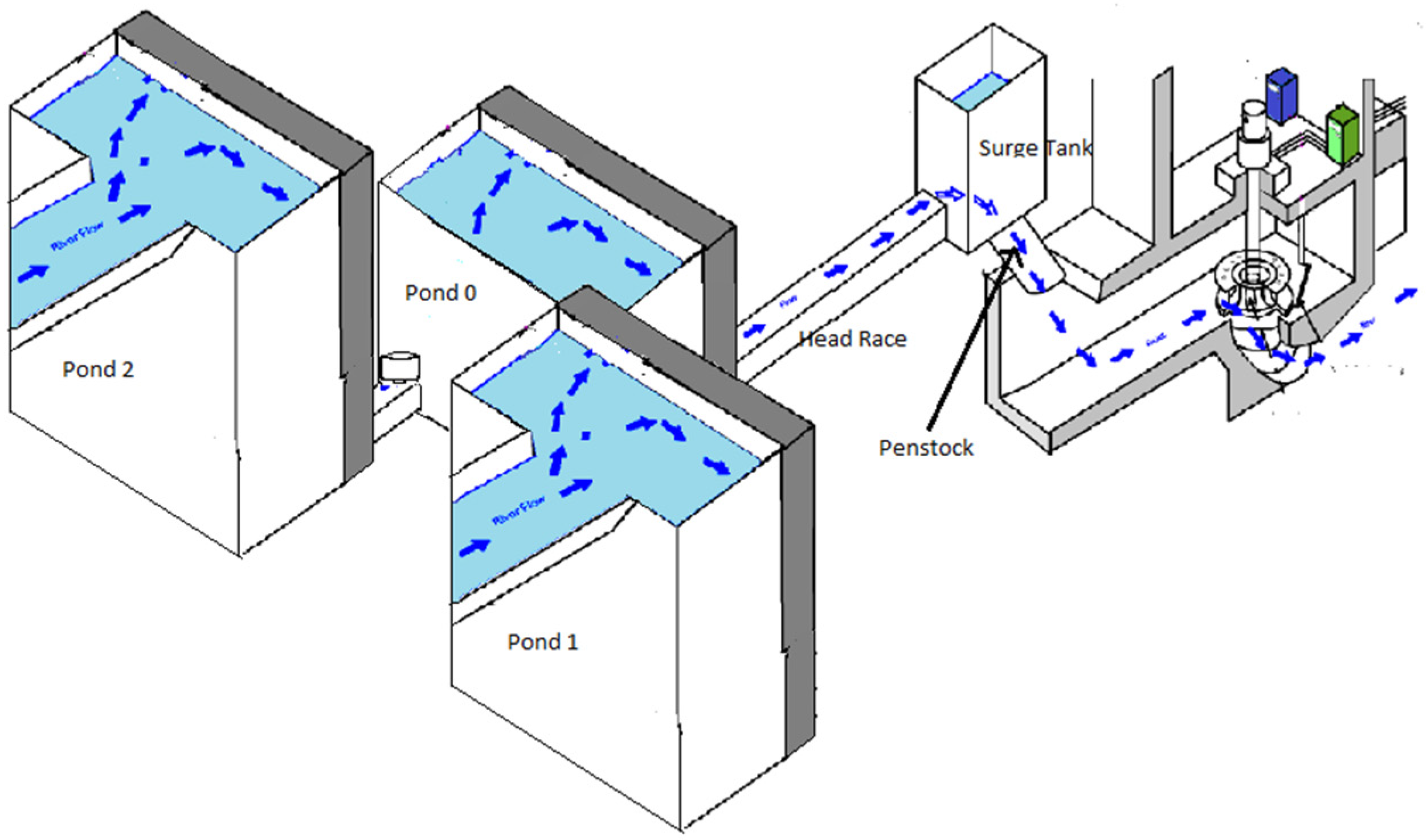
The system considered here is a redirected run-of-river hydropower plant, which is discussed in [1]. The hydraulic part of the plant consists of three head ponds, pond 1 $(T_1)$, 2 $(T_2)$, and 0 $(T_0)$. Water from the river enters ponds 1 and 2. Ponds 1 and 2 are connected at the bottom to the head pond 0 through tunnels. Both tunnels from pond 1 to pond 0 and pond 2 to pond 0 have a controllable valve, $s_1$ and $s_2$, respectively. The head pond 0 is connected from the bottom to the surge tank $T_s$ through the long headrace tunnel. The level of water of the ith pond is denoted by $x_i$. Figure 1 shows the construction of the system.

The equations describing the hydraulic part will be discussed according to [1]. A modification in the model will be proposed, and its interaction with a Francis turbine will be discussed. The head ponds are described by the rate of change of their water levels. The rate of change of the water level is a function of its area and the net difference of the outflows and inflows. For pond 1 the equation is given by [1].

$$\frac{d}{dt}{x}_1=-\frac{ȵa}{A}{s}_1\sqrt{2g\left|x_1-x_0\right|}sgn\left(x_1-x_0\right)+\frac{U_1}{A}$$

(1)

where $x_1$ is the water level in pond 1, and $A$ is the cross-sectional area of the pond. The duct connecting ponds 1 and 0 have a cross-sectional area,$a$. The controllable valve $s_1$ is between ponds 1 and 0. The constants are $ȵ$, the dimensionless water flow constant of value 0.98 [16], and $g$, the gravitational constant of $9.8\raisebox{1ex}{$m$}\!\left/ \!\raisebox{-1ex}{$s^2$}\right.$.

In Equation (1), $sgn\left(z\right)$ is defined as

$$sgn\left(z\right)=\{\begin{array}{cc}1& z>0\\ 0& z=0\\ -1& z<0\end{array}$$

(2)

and $\left|z\right|$ is

$$\left|z\right|=\{\begin{array}{cc}z& z\ge 0\\ -z& z<0\end{array}$$

(3)

Furthermore, note that the flow between two tanks or ponds depends on the difference in the levels between them and the cross-sectional area of the duct connecting them.

Similarly, the equation describing the rate of change in the water level in pond 2 is

$$\frac{d}{dt}{x}_2=-\frac{ȵa}{A}{s}_2\sqrt{2g\left|x_2-x_0\right|}sgn\left(x_2-x_0\right)+\frac{U_2}{A}$$

(4)

In ponds 1 and 2, the river’s inflow is assumed controllable, whereas the outflow is to pond 0. The dynamics of pond 0 are described by the following equation.

$$\frac{d}{dt}{x}_0=\frac{ȵa}{A}\lceil s_1\sqrt{2g\left|x_1-x_0\right|}sgn\left(x_1-x_0\right)+s_2\sqrt{2g\left|x_2-x_0\right|}sgn\left(x_2-x_0\right)\rceil -\frac{Q_t}{A}$$

(5)

The equation describing the dynamics of the headrace is the same as the rate of flow in a tube, which depends on the difference in the water levels at both ends, its cross-sectional area, and the tube’s length. The flow frictional losses are also accounted for by subtracting them from the expression. Therefore, the rate of flow of water in the headrace is given by

$$\frac{d}{dt}{Q}_t=\frac{g{A}_t}{L_t}\left(x_0-x_s\right)-C_t{Q}_t\left|Q_t\right|$$

(6)

where $Q_t$ is the flow of water through the headrace, $A_t$ is the headrace’s cross-sectional area, and $L_t$ is the length of the headrace.

For the surge tank, the rate of change in its level $x_s$ is given by

$$\frac{d}{dt}{x}_s=\frac{Q_t}{A_s}-\frac{ȵa}{A_s}\sqrt{2g{x}_s}$$

(7)

where $A_s$ is the cross-sectional area of the surge tank. The above Equations (1) and (4)–(7) describe the system from [1]. Note also that the control variables are $U_i$, where $i=1,2$. $U_i$ is the controllable flow of river into the pond $i$ and is varied between a maximum value and zero. The other control variables are $s_j$, where $j=1,2$. $s_j$ is the controllable valve between ponds. $s_1$ is the valve between pond 1 and 0 while $s_2$ is the valve between pond 2 and 0. The valve $s_j$ can be varied between zero and unity.

We have proposed two modifications to the above mentioned system. The first one is a modification to the flow of water entering ponds 1 and 2 and the second is to couple it with a turbine.

In [1], it is assumed that the inflow of river in ponds 1 and 2 are completely controllable; however, this is not practically achievable. The flow of the river can be controlled by adding a gate in its path. The river flow can have some short and long-term variations and some base flow rates. For simplicity, the river’s flow is taken as a combination of the constant base flow rate and short-term variable flow rate and is modeled by a sinusoidal function. In contrast, the long-term variation is considered constant and is included in the base flow rate. Therefore, the flow rate in cubic meter per second of the river is given by

$$l=m+p \sin \omega t$$

(8)

where $l$ is the total flow rate, $m$ is the baseline constant flow rate, and $p \sin \omega t$ is the short-term variation in the flow rate. It is assumed that a controllable sluice gate $w$ is present at the mouth of the pond from the river. Now, $U$ is the controllable flow rate from [1], and is given by

$$U=wl$$

(9)

where $w$ ranges from 0 to 1. Now, as a turbine with penstock is added to the hydraulic system, Equation (7) of the surge tank is modified. The out flow from the surge tank is changed to be a single variable instead of the expression. The outflow from the surge tank and inflow to the penstock and turbine is denoted by $Q$ as

$$ȵa\sqrt{2g{x}_s}=Q$$

(10)

Now one substitutes the river and turbine flow values in the model and rewrite the equations. After substituting Equation (9) in Equations (1) and (4), the equations for pond 1 and 2 become

$$\frac{d}{dt}{x}_1=-\frac{ȵa}{A}{s}_1\sqrt{2g\left|x_1-x_0\right|}sgn\left(x_1-x_0\right)+\frac{w_1{l}_1}{A}$$

(11)

$$\frac{d}{dt}{x}_2=-\frac{ȵa}{A}{s}_2\sqrt{2g\left|x_2-x_0\right|}sgn\left(x_2-x_0\right)+\frac{w_2{l}_2}{A}$$

(12)

Note that $U_1$ and $U_2$ are replaced by $w_1{l}_1$ and $w_2{l}_2$, which is the product of the river flow and the sluice gate opening into ponds 1 and 2. The equations for pond 0 and the headrace are unchanged.

$$\frac{d}{dt}{x}_0=\frac{ȵa}{A}\lceil s_1\sqrt{2g\left|x_1-x_0\right|}sgn\left(x_1-x_0\right)+s_2\sqrt{2g\left|x_2-x_0\right|}sgn\left(x_2-x_0\right)\rceil -\frac{Q_t}{A}$$

(13)

$$\frac{d}{dt}{Q}_t=\frac{g{A}_t}{L_t}\left(x_0-x_s\right)-C_t{Q}_t\left|Q_t\right|$$

(14)

Finally, the equation of the surge tank is modified by plugging in Equation (10) in Equation (7) as

$$\frac{d}{dt}{x}_s=\frac{Q_t}{A_s}-\frac{Q}{A_s}$$

(15)

Therefore, the system equations from the [1] are modified for the current system. The inputs of the system are

$$\overrightarrow{v}={\left[\begin{array}{ccc}{U}_1& U_2& \begin{array}{ccc}{s}_1& s_2& Q\end{array}\end{array}\right]}^T$$

(16)

where $Q$ is the flow through the turbine and is dictated by the equations of the turbine, while the rest of the inputs of the system are the control variables which are given as

$$\overrightarrow{u}={\left[\begin{array}{cc}{U}_1& \begin{array}{ccc}{U}_2& s_1& s_2\end{array}\end{array}\right]}^T$$

(17)

Note also that $U_1,U_2$ are given by the level controller, which is discussed in the next section and is equated using Equation (9).

Comparing the above Equations (16) and (17), the input of the system is

$$\overrightarrow{v}={\left[\begin{array}{cc}{\overrightarrow{u}}^T& Q\end{array}\right]}^T$$

(18)

The states vector $\overrightarrow{x}$ consisting of the state variables is

$$\overrightarrow{x}={\left[\begin{array}{ccc}{x}_1& x_2& \begin{array}{ccc}{x}_0& Q_t& x_s\end{array}\end{array}\right]}^T$$

(19)

The output of the hydraulic system is

$$\overrightarrow{y}=C\overrightarrow{x}$$

(20)

where the matrix $C$ is given by

$$C=\left[\begin{array}{cc}\begin{array}{ccc}0& 0& 1\\ 1& 0& 0\end{array}& \begin{array}{cc}0& 0\\ 0& 0\end{array}\\ \begin{array}{ccc}0& 1& 0\\ 0& 0& 0\end{array}& \begin{array}{cc}0& 0\\ 0& 1\end{array}\end{array}\right]$$

(21)

Resultantly $\overrightarrow{y}$ becomes:

$$\overrightarrow{y}={\left[\begin{array}{ccc}{x}_0& x_1& \begin{array}{cc}{x}_2& x_s\end{array}\end{array}\right]}^T$$

(22)

After the formulation of the hydraulic system model, the model of the turbine and penstock is needed to complete the hydropower system. In this work, the three-pond hydraulic system has a Francis turbine and penstock taken from [2]. The Francis turbine is described as a function of its rotational speed $n$ and gate opening $G$to achieve a flow rate $Q$. The equation for the flow of water from the turbine is given as

$$Q=h\left(G,n\right)$$

(23)

The characteristics of a Francis turbine are described by a set of points described by hill graphs [15]. For Hill graphs, a predetermined operating point of the turbine is set, and then the static values of $G$ and $n$ are used in the calculations. However, [2] describes the characteristics of the turbine in the form of a quadratic equation that is non dimensional. In addition to providing a dynamic model of the Francis turbine, this model is also completely scalable over different operating conditions and rated values. The equation for the Francis turbine from [2] is described as

$$\frac{Q}{Q_r}=G\left[a_1\frac{n^2}{n_r^2}+b_1\frac{n}{n_r}+c_1\right]$$

(24)

where $n_r$and $Q_r$ are the rated speed and the rated flow rate of the turbine, and the constants $a_1,b_1,c_1$ are the constants within the above quadratic equation, as stated by [2]. The torque generated by the turbine is given by the following equation [2].

$$\frac{M}{M_r}=\frac{\frac{Q}{Q_r}\frac{H}{H_r}}{\frac{n}{n_r}}$$

(25)

where $M$ and $M_r$ are the torque and rated torque. $H$ and $H_r$ are the height or level of water and the rated height, respectively. In the case of our system, the level or height ($H$) of concern is $x_0$ and the rated height ($H_r$) is the height of the pond 0 so the rated height is $H_0$.

Now, rewriting Equation (25)for the generated torque of the turbine in our system, we get

$$\frac{M}{M_r}=\frac{Q}{Q_r}\frac{x_0}{H_0}\frac{n_r}{n}$$

(26)

The power generated at the turbine is given by the product of rotational speed and torque of the turbine as in [2]:

$$P=nM$$

(27)

The total output of the system is the output of the hydraulic system and power.

$$\overrightarrow{Y}={\left[\begin{array}{ccc}{x}_0& x_1& \begin{array}{ccc}{x}_2& x_s& P\end{array}\end{array}\right]}^T$$

(28)

We shall be requiring the explicit values of $\overrightarrow{Y}$ in order to conveniently find the effects of the faults on the output. As the faults occur, we diagnose them by computing the values of the states by integrating the state equations rather than just taking the output value. The value of $x_0$ is computed by integrating Equation (13).

$$x_0=\frac{ȵa}{A}{{\displaystyle \int }}_0^t\lceil s_1\sqrt{2g\left|x_1-x_0\right|}sgn\left(x_1-x_0\right)+s_2\sqrt{2g\left|x_2-x_0\right|}sgn\left(x_2-x_0\right)\rceil dt-{{\displaystyle \int }}_0^t\frac{Q_t}{A}dt$$

(29)

Similarly, for $x_1$, $x_2$, and $x_s$, Equations (11), (12), and (15) are integrated.

$$x_1=-\frac{ȵa}{A}{{\displaystyle \int }}_0^t{s}_1\sqrt{2g\left|x_1-x_0\right|}sgn\left(x_1-x_0\right)dt+{{\displaystyle \int }}_0^t\frac{w_1{l}_1}{A}dt$$

(30)

$$x_2=-\frac{ȵa}{A}{{\displaystyle \int }}_0^t{s}_2\sqrt{2g\left|x_2-x_0\right|}sgn\left(x_2-x_0\right)dt+{{\displaystyle \int }}_0^t\frac{w_2{l}_2}{A}dt$$

(31)

$$x_s={{\displaystyle \int }}_0^t\frac{Q_t}{A_s}dt-{{\displaystyle \int }}_0^t\frac{Q}{A_s}dt$$

(32)

Furthermore, power is calculated by Equation (27), and we plug the value of the torque from Equation (26) into Equation (27) after simplifying.

$$P=\frac{Q{M}_r{x}_0{n}_r}{Q_r{H}_0}$$

(33)

Now, plugging in the value of $Q$ from Equation (24) to Equation (33) and simplifying.

$$P=\frac{M_r{x}_0{n}_r}{H_0}G\left[a_1\frac{n^2}{n_r^2}+b_1\frac{n}{n_r}+c_1\right]$$

(34)

Although this step appears to be an unnecessary complication, it will help us find the residues easily in case of faults.

3. Control Design

The control system for the system is done in a pseudo hierarchal and nested style. There are three levels of control dealing with level control, level reference, and gate (power) control. Now, these three controls will be discussed separately. The simplified form of the control system with the three levels of control is given in Figure 2.

3.1. Level Controller

The primary level control governs the hydraulic part of the system. The primary level control is discussed in [1]. Level control has the controllable variables $s_1$,$s_2$, and $U_1$, $U_2$.$s_1$ is the valve between pond 1 and 0 while $s_2$ is the valve between pond 2 and 0. While $U_1$and $U_2$are the flow of river in the ponds 1 and 2 through the sluice gates. In this work’s current scheme, the level control is essentially the same as in [1], with two differences. The first difference is discussed in the previous section regarding the controllable flow of river in the ponds 1 and 2. While the next change is just that the reference levels of the three ponds are set at the same level by the reference control, as opposed to [1], in which all the reference levels could be set at different levels. Combining Equations (1) and (4)–(7) of the hydraulic system gives us the nonlinear system of equations as

$$\frac{d}{dt}\overrightarrow{x}=\overrightarrow{f}\left(\overrightarrow{x},\overrightarrow{u}\right)$$

(35)

where the state variables are

$$\overrightarrow{x}={\left[\begin{array}{ccc}{x}_1& x_2& \begin{array}{ccc}{x}_0& Q_t& x_s\end{array}\end{array}\right]}^T$$

(36)

and the control variables are

$$\overrightarrow{u}={\left[\begin{array}{cc}{U}_1& \begin{array}{ccc}{U}_2& s_1& s_2\end{array}\end{array}\right]}^T$$

(37)

Here, $U_1,U_2$ range from 0 to $U_{Max}$ and $s_1,s_2$ range from 0 to 1. However, in the current system the flow $U$ is equal to the product of the flow-rate of the river $l$ and the opening of the sluice gate $w$, as shown in Equation (9). The controller gives $U_1,U_2$, the required flow-rate output to maintain the ponds’ water levels at the desired reference level. According to Equation (9):

$$U_i=l_i{w}_i$$

(38)

where $i=1,2$ for ponds 1 and 2. We have control input $U_i$ and river flow rate $l_i$ from the river. We control the sluice gate by the expression

$$w_i=\{\begin{array}{cc}\frac{U_i}{l_i}& \frac{U_i}{l_i}\le 1\\ 1& \frac{U_i}{l_i}>1\end{array}$$

(39)

This ensures that $U_i$ cannot exceed $l_i$, the actual flow-rate in the river; the actual controlled system is slightly slower to reach its steady state as compared to [1], as it makes a more realistic approach towards the problem.

A fuzzy controller is used for level control due to its flexibility and ease of controlling different nonlinear and complex applications. Another advantage is its speed and higher accuracy compared to traditional PID controllers. A fuzzy controller is a linguistic and intuitive controller as it takes the input in the form of linguistic variables and gives output in the same way. A fuzzy system consists of a set of IF-THEN rules. In the first part, the input variable is a crisp value that is fuzzified to convert it into a linguistic variable. The system takes input in the form of linguistic variables. It then gives output in the form of a linguistic variable for the Mamdani type system or a linear combination of inputs for a Takagi Sugeno type system. Similarly, the output linguistic variable is defuzzified to convert it into the crisp output. For example, a two-input fuzzy system will have a rule of this form:

$$Rule 1: IF x_{1 }is A_{1 }^1 and x_{2 }is A_{2 }^{1}THEN y is B^1$$

(40)

As shown in Figure 2, level control is driven by the state errors and the states of the hydraulic system. The actual level control is the same as [1] and is done using Mamdani fuzzy control. The level reference is given by the level reference control, which is discussed next. The levels $x_{1 }{x}_{2 }{x}_{0 }$ of the ponds 1, 2, and 0 are given the membership functions Low, Medium, and High. Similarly, the membership functions of the errors $E_{1 }{E}_{2 }{E}_0$ are given as Negative, Near Zero, and Positive. The outputs have five membership functions each, from $L_0$ to $L_4$, with $L_0$ indicating the complete closure of the valve or river water input, while $L_4$means full throttle. The number of rules for the system depends on the number of inputs and the total number of membership functions. So, there are six membership functions for each of the three ponds. The total possible rules are 729, the same as the total possible combinations, which is rather computationally intensive. Therefore, the level control is divided into two parts. One control is for pond 1 and 0, while the second control is for ponds 2 and 0. Dividing the control in two parts reduces the number of rules to 81 for each controller. It may appear that a clash may theoretically exist between level control 1 and 2, but as the level reference of pond 0 is the same for both controls, no such clash exists. Although this level control can maintain the ponds at different levels, as discussed in [1], all the three references are set at the same level by the level reference controller. The controllable variables are the valve position $s$ and the inflow $U$, which are nonzero numbers ranging from 0 (close) to full throttle. Therefore, the levels are adjusted by balancing the inflows and the outflows to increase, decrease, and maintain the ponds’ levels. Depending on the required levels of the three ponds, the controller can achieve and maintain the water levels in the ponds. In the current case, the reference controller sets the reference levels of all three ponds at the same level. The controller currently does not use the level controller’s ability to achieve and maintain the water levels at different levels.

We shall consider one of the two controllers for discussion as the second controller mirrors the first. The Mamdani controller works in three main modes, each for when the current levels are below, on, or higher than the required levels. When the actual level is lower than the required level in the ponds, the sluice gate (inflow) is set to maximum or high so that pond 1 reaches the required level. The valve $s_1$ is kept at full throttle, so that pond 0 also reaches the required level. When errors are near zero, both the inflow and the valve $s_1$are kept at level 1 where inflows and outflows are balanced and the water level is retained in the ponds. Finally, if the actual water level exceeds the required level, the inflow is stopped, and valve $s_1$ is kept at full throttle so that the levels reduce and reach the required level. Another small addition to this is that the controller prioritizes the level of pond 0. That means if somehow the level of pond 1 is increased due to some disturbance or unknown noise, the disturbance will not appear in pond 0 as the controller prioritizes the level of pond 0. The controller does not allow pond 1 to decrease to the required level if it means to increase the level of pond 0 above its required level. An example of the rule when the system is in an equilibrium state is given below:

$$\begin{gathered} IF E1 is ZERO and E0 is ZERO and X1 is HIGH and X0 is HIGH \\ THEN U1 is L1 and S1 is V1 \end{gathered}$$

(41)

All of the 81 rules for each level controller 1 and 2 have a generalized form:

$$u\left(t\right)=\frac{{{\displaystyle \sum }}_{j=1}^{81}{\overline{u}}_j\left({{\displaystyle \prod }}_i^4{\mu }_{A_i^j}\left(k_i\right)\right)}{{{\displaystyle \sum }}_{j=1}^{81}\left({{\displaystyle \prod }}_i^4{\mu }_{A_i^j}\left(k_i\right)\right)}$$

(42)

where $u\left(t\right)$ is the controller’s output for $U_1$ or $s_1$, $k_i$ is the input value of $x_0,x_1,E_0$, and $E_2$. The linguistic variable for input, which can be $NEG,ZERO,POS$ or $LOW, MED,HI$, is $A$; ${\mu }_A$ is the membership function of $A$; and ${\overline{u}}_j$ is the firing strength of the $j^{th}$ fuzzy rule.

3.2. Level Reference Controller

The second controller that controls both the hydraulic system and turbine is also a fuzzy controller. The reference controller takes the input in the form of required power and the level of the pond 0. This controller requires the exact value of the required power or at least a scaled version of it. Therefore, the hydraulic system parameters are taken from [1], and the parameters of the hydraulic turbine are taken arbitrarily to match with the hydraulic system. After that, the total theoretical power is calculated, which comes around 2 Mega Watts of power. Next, the minimum level of the pond is also decided arbitrarily as it is very rare for the head pond of a power plant to be empty. That minimum level and minimum power are arbitrarily decided as 20 m and 800 kilo watts.

The reference controller does not run the errors as opposed to the level controller but with the reference power and the feedback from the pond 0 (level). The head ponds’ operating levels range from 20 m to a maximum of 35 m [1], and the operating power is between 800 kW and 2 MW.

The reference controller is in the form of the Takagi Sugeno Fuzzy Inference Engine instead of Mamdani Fuzzy Inference Engine for the previously discussed level controller. The Takagi Sugeno controller is different from the Mamdani controller in the form as its output is a constant or a linear combination of its inputs for each rule.

The function of the reference controller is to set a level reference for the ponds and give the initial base position to the gate of the turbine. As the power plant operates between 800 kW and 2 MW and from the 20 to 35 m pond level, the available power for the turbine is given by the following equation:

$$P=\eta \rho gHQ$$

(43)

where $\eta$ is the turbine efficiency, $\rho$ is the density of water, $g$ is the gravitational constant, and $H$and $Q$are the level of water in pond and the flow rate through the turbine, respectively. As the efficiency of the turbine is not in our control, as the model taken from [2] assumes constant efficiency for the turbine, and the density of water and gravitational constants are fixed, the level of the water in head pond and the flow rate through the turbine can be adjusted. According to Equation (34), the turbine’s rotational speed can also be used as a control parameter, but we kept it constant and is left for future work. The flow rate through the turbine is adjusted by adjusting the opening of the turbine wicket gate. The pond level is divided from 20 m to 35 m in increments of 1 m, and the operating power is adjusted from 800 kW to 2 MW in increments of 25 kW. The position of the turbine gate is estimated against the required power and water level while fixing the other parameters. This estimation is the basis for the rules of level reference and initial gate position of the turbine.

The inputs of the level reference control are the required power and the level of pond 0. These inputs are assigned membership functions as follows: The pond level can be varied from 20 to 35 m, so the level is assigned four membership functions. The first membership function deals with levels less than 20 m, while the rest three deal with from 20 to 35 m in increments of 5 m. The level membership functions are named as $m_{20}$, $m_{25}$, $m_{30}$, and $m_{35}$, respectively. All four level membership functions are trapezoidal, with the first membership function being non symmetric to describe all the levels less than 20 m. The required power level $\left(REQP\right)$ is divided into increments of 25 kW between 800 kW and 1.95 MW. That means that 45+2 membership functions describe the required power. The 45 membership functions are between 800 kW and 1.95 MW, while the other two represent power levels less than 800 kW and greater than 1.95 MW. The inner 45 membership functions are triangular, while the boundary membership functions are trapezoidal. Therefore, the total number of rules for the level reference controller is 4 × 47 or 188. The controller requires the current level of the head pond to give the level reference; for when the required power level is reduced, and the current level of the pond is higher than the theoretical level, to stop the controller from quickly reducing the level of the pond. The other aspect to know about the current level is to set the initial position of the turbine gate according to the current level rather than the desired level. An example of a rule is given below.

$$IF REQP is 165P and LEVEL is m_{25} THEN LEVREF is 30 and G_{Fuzzy} is 0.92$$

(44)

All of the 188 rules for the level reference controller have a generalized form:

$$u\left(t\right)=\frac{{{\displaystyle \sum }}_{j=1}^{188}{\overline{u}}_j\left({{\displaystyle \prod }}_i^2{\mu }_{A_i^j}\left(k_i\right)\right)}{{{\displaystyle \sum }}_{j=1}^{188}\left({{\displaystyle \prod }}_i^2{\mu }_{A_i^j}\left(k_i\right)\right)}$$

(45)

where $u\left(t\right)$ is the output of the controller for $LEVREF$ or $G_{Fuzzy}$, $k_i$is the input value of $REQP$ and $LEVE$. The linguistic variable for the input, which has been described above is, $A$; ${\mu }_A$ is the membership function of $A$; and ${\overline{u}}_j$ is the firing strength of the jth fuzzy rule.

3.3. Turbine Gate Correction Control

The turbine gate correction control is the final fine adjustment control for the turbine gate. The level reference control discussed earlier gives the required level to the level control and gives the turbine gate’s initial gate position. The final adjustment to the turbine gate is made using a traditional PID controller. The output of the PID controller is added to the previously assigned initial position of the gate by the level reference controller. Therefore, the final value of the turbine gate becomes

$$G_{FINAL}=G_{Fuzzy}+G_{PID}$$

(46)

The PID control is a traditional control scheme that is driven by the error between the required power and generated power, and the output of controller is given by

$$G_{PID}=K_{P}e\left(t\right)+K_I{{\displaystyle \int }}_0^{t}e\left(t\right)dt+K_D\frac{d}{dt}e\left(t\right)$$

(47)

where $e\left(t\right)$ is the power error, and $K_P$, $K_I$, and $K_D$ are the proportional, integral, and derivative constants of the PID controller.

By the interaction of these three controllers, the required levels of the ponds are maintained, and the generated power comes within a hundred watts of the required power.

4. Fault Model

A few commonly occurring faults were modeled and added to the system to make fault diagnostics and a fault-tolerant control. These faults were added to the system model, detected, and identified by the fault diagnostic module, and then suggested fault-tolerant control action is taken. In this work, currently, only saturation and leakage faults are considered.

The saturation and leakage faults most commonly occur within the valves and gates due to age, obstruction, or a weakened or faulty actuator. Saturation fault occurs when the actuator cannot fully open the valve or gate; this reduces flow which is amplified by propagating through the system and affects the output by making it sluggish or having lower than the desired value. Similarly, a leakage fault is the same as but opposite to a saturation fault. During a leakage fault, the gate or valve cannot close or shut completely, resulting in a constant leakage, having the output creeping higher than the desired value, or having a sluggish response when braking or lowering the desired states of the system. During the normal mode of operation (i.e., from zero or lower initial conditions to higher desired states), the effects of saturation fault appear during the transient state but are not present during the steady state. In comparison, the case is vice-versa for leakage faults where their effects appear in the steady state but are invisible in the transient state. Although this rule is not strictly followed, and it will be seen later when these faults are added to the system. As a general rule of thumb, the faults whose effects appear in the steady state are more severe than those whose effects only appear during the transient state.

From a purely fault-tolerant point of view, the faults whose effects are only present during the transient state may not strictly require corrective action. As in this case, the system is merely somewhat slower than a normal system unless it is so slow that it becomes undesirable. In comparison, a fault whose effect is evident in the steady state has to be dealt with using corrective action to keep the undesirable effects of the faults to a minimum. However, detecting, identifying, and isolating both kinds of faults are very important for early warning and avoiding the system from failing.

If we consider a single equation for a generalized linear system, then

$$\dot{x}=Ax+Bu$$

(48)

where $A$ is the state gain matrix and $B$ is the input gain matrix. In case of the occurrence of a fault, the equation is modified as follows:

$$\dot{x}=Ax+Bu+Ef$$

(49)

where $E$ is the fault gain and $f$ is the fault. In case of a nonlinear system with a nonlinear fault, the system becomes

$$\dot{x}=g\left(x,u,f\right)$$

(50)

Now let us consider our system equations and see how they are affected by the faults. The types of faults being considered are saturation, leakage, and a combination of the two. The components affected by these faults are the sluice gates $w_1$ and $w_2$, which allow the river’s flow in ponds 1 and 2, the controllable valves $s_1$and $s_2$between the ponds $T_1$, $T_0$ and $T_1$, $T_0$, and finally, the wicket gate $G$ of the Francis turbine. Sometimes the nonlinear fault can be separated as an additive or a multiplicative function, which is sometimes not easily possible. First, let us describe the faults mathematically before finding their effect on the components. The saturation fault, nonlinear in nature, is described as

$$f^1\left(z\right)=\{\begin{array}{cc}z& z<Sat\\ Sat& z\ge Sat\end{array}$$

(51)

where $z$ is an arbitrary faulty component, and $Sat$ is the constant saturation limit of the effect of the fault. However, plugging this value of fault into the system is not feasible. Therefore, we transform this nonlinear fault as an additive fault to the system. The additive effect may be time varying or nonlinear, as is needed by the system. The fault $f^1$ is described in its additive form as

$$f^1\left(z\right)=\{\begin{array}{cc}z& z<Sat\\ z+f_z^1& z\ge Sat\end{array}$$

(52)

In the term $f_z^1$, $z$ is the faulty component and $f_z^1$ is the time varying term that satisfies the equation below.

$$z+f_z^1=Sat$$

(53)

Similarly, the leakage fault is defined as

$$f^2\left(z\right)=\{\begin{array}{cc}Leak& z<Leak\\ z& z\ge Leak\end{array}$$

(54)

Here, $Leak$ is the constant leakage effect of the fault. Now, one can describe the leakage fault in additive form as

$$f^2\left(z\right)=\{\begin{array}{cc}z+f_z^2& z<Leak\\ z& z\ge Leak\end{array}$$

(55)

The time-varying term $f_z^2$ satisfies the following equation:

$$z+f_z^2=Leak$$

(56)

Similarly, when these two types of faults occur at the same time, it is defined as $f^3$, which is defined as

$$f^3\left(z\right)=\{\begin{array}{cc}Sat& z>Sat\\ z& Leak\le z\le Sat\\ Leak& z<Leak\end{array}$$

(57)

To describe the $f^3$ type of fault, $f_z^3$ is not needed, as shown in the additive form of the fault below.

$$f^3\left(z\right)=\{\begin{array}{cc}z+f_z^1& z>Sat\\ z& Leak\le z\le Sat\\ z+f_z^2& z<Leak\end{array}$$

(58)

The above equations from Equation (51) to Equation (58) shall be referred to multiple times to define $f_z^i$, where the faulty component is $z$ and $i=1,2$, depending on whether the component is in saturation or leakage fault. This will be used extensively to convert the fault equations into additive forms.

Now let us look at how these faults affect the components of the system. We shall examine the sluice gate, pond valve, and turbine wicket gate fault one by one. There are two sluice gates and pond valves; only one of each will be examined to avoid redundancy.

4.1. Sluice Gate Faults

The sluice gates are on the opening of the river to the ponds $T_1$ and $T_2$. Although, the level controller assumes that the flow of the river into the ponds is controllable explicitly, the sluice gates $w_1$ and $w_2$ control the inflow by monitoring the river flow using Equation (38). The equation for pond 1 $T_1$, Equation (11), is rewritten adding the effect of fault $f^1$ below.

$$\frac{d}{dt}{x}_1=-\frac{ȵa}{A}{s}_1\sqrt{2g\left|x_1-x_0\right|}sgn\left(x_1-x_0\right)+\frac{f^1(w_1)l_1}{A}$$

(59)

According to Equation (52), the effect of the sluice gate fault in the saturation region can be written as a sum with the $f_{w_1}^1$ term. When the effect of the $f^1$ fault appears for the sluice gate, Equation (57) is written as

$$\frac{d}{dt}{x}_1=-\frac{ȵa}{A}{s}_1\sqrt{2g\left|x_1-x_0\right|}sgn\left(x_1-x_0\right)+\frac{w_1{l}_1}{A}+\frac{f_{w_1}^1{l}_1}{A}$$

(60)

Note that the value of $f_{w_1}^1$ is negative in the above case. To find the fault’s total effect, we integrate the above Equation (60).

$$x_1=-\frac{ȵa}{A}{{\displaystyle \int }}_0^t{s}_1\sqrt{2g\left|x_1-x_0\right|}sgn\left(x_1-x_0\right)dt+{{\displaystyle \int }}_0^t\frac{w_1{l}_1}{A}dt+{{\displaystyle \int }}_0^t\frac{f_{w_1}^1{l}_1}{A}dt$$

(61)

Similarly, for the case of a leakage fault, the equation becomes

$$\frac{d}{dt}{x}_1=-\frac{ȵa}{A}{s}_1\sqrt{2g\left|x_1-x_0\right|}sgn\left(x_1-x_0\right)+\frac{f^2(w_1)l_1}{A}$$

(62)

Going through similar steps and defining $f_{w_1}^2$ the fault $f^2$ is converted to an additive form and the effect of the fault in leakage mode is written as

$$\frac{d}{dt}{x}_1=-\frac{ȵa}{A}{s}_1\sqrt{2g\left|x_1-x_0\right|}sgn\left(x_1-x_0\right)+\frac{w_1{l}_1}{A}+\frac{f_{w_1}^2{l}_1}{A}$$

(63)

The total effect of the fault is given by integrating the above Equation (63) as before:

$$x_1=-\frac{ȵa}{A}{{\displaystyle \int }}_0^t{s}_1\sqrt{2g\left|x_1-x_0\right|}sgn\left(x_1-x_0\right)dt+{{\displaystyle \int }}_0^t\frac{w_1{l}_1}{A}dt+{{\displaystyle \int }}_0^t\frac{f_{w_1}^2{l}_1}{A}dt$$

(64)

Using the similar reasoning the effect of third type of fault appears in the equation as

$$\frac{d}{dt}{x}_1=-\frac{ȵa}{A}{s}_1\sqrt{2g\left|x_1-x_0\right|}sgn\left(x_1-x_0\right)+\frac{f^3(w_1)l_1}{A}$$

(65)

Since the $f^3$ fault is a combination of the saturation and leakage faults, the additive form of the fault $f^3$ on the sluice gate $w_1$ is described by Equations (61) and (64), depending on whether the fault is in the saturation or leakage region. The fault model for $w_2$ is the same as above and discussing it will be redundant.

4.2. Pond Valve Fault

In the case of a fault in the valve $s_1$, its effect appears in two equations. The equations are of pond 1 and pond 0. The equation for pond 1, Equation (11), with the occurrence of fault $f^1$, is modified as follows:

$$\frac{d}{dt}{x}_1=-\frac{ȵa}{A}{f}^1(s_1)\sqrt{2g\left|x_1-x_0\right|}sgn\left(x_1-x_0\right)+\frac{w_1{l}_1}{A}$$

(66)

Similarly, the equation for the head pond 0 (13) is modified as follows

$$\frac{d}{dt}{x}_0=\frac{ȵa}{A}\lceil f^1 \left(s_1\right)\sqrt{2g\left|x_1-x_0\right|}sgn\left(x_1-x_0\right)+s_2\sqrt{2g\left|x_2-x_0\right|}sgn\left(x_2-x_0\right)\rceil -\frac{Q_t}{A}$$

(67)

Rewriting the faults in additive form according to Equation (50) and defining $f_{s_1}^1$, the equation for pond 1 in the saturation fault region is

$$\begin{gathered} \frac{d}{dt}{x}_1=-\frac{ȵa}{A}{s}_1\sqrt{2g\left|x_1-x_0\right|}sgn\left(x_1-x_0\right)-\frac{ȵa}{A}{f}_{s_1}^1\sqrt{2g\left|x_1-x_0\right|}sgn\left(x_1-x_0\right) \\ +\frac{w_1{l}_1}{A} \end{gathered}$$

(68)

Likewise, the equation for pond 0 during the saturation region of the fault is

$$\begin{gathered} \frac{d}{dt}{x}_0=\frac{ȵa}{A}\lceil s_1\sqrt{2g\left|x_1-x_0\right|}sgn\left(x_1-x_0\right)+f_{s_1}^1\sqrt{2g\left|x_1-x_0\right|}sgn\left(x_1-x_0\right) \\ +s_2\sqrt{2g\left|x_2-x_0\right|}sgn\left(x_2-x_0\right)\rceil -\frac{Q_t}{A} \end{gathered}$$

(69)

The total effect of the fault on pond 1 is given by integrating Equation (68).

$$\begin{gathered} x_1=-\frac{ȵa}{A}{{\displaystyle \int }}_0^t{s}_1\sqrt{2g\left|x_1-x_0\right|}sgn\left(x_1-x_0\right)dt \\ -\frac{ȵa}{A}{{\displaystyle \int }}_0^t{f}_{s_1}^1\sqrt{2g\left|x_1-x_0\right|}sgn\left(x_1-x_0\right)dt+{{\displaystyle \int }}_0^t\frac{w_1{l}_1}{A}dt \end{gathered}$$

(70)

Similarly, the total effect of fault on pond 0 is given by integrating Equation (69).

$$\begin{gathered} x_0=\frac{ȵa}{A}{{\displaystyle \int }}_0^t\lceil s_1\sqrt{2g\left|x_1-x_0\right|}sgn\left(x_1-x_0\right)+f_{s_1}^1\sqrt{2g\left|x_1-x_0\right|}sgn\left(x_1-x_0\right) \\ +s_2\sqrt{2g\left|x_2-x_0\right|}sgn\left(x_2-x_0\right)dt\rceil -{{\displaystyle \int }}_0^t\frac{Q_t}{A}dt \end{gathered}$$

(71)

We shall be delving more deeply into the effects of the saturation fault of the pond valve in the Appendix A. Using similar reasoning as above, the occurrence of fault $f^2$ on the valve $s_1$ modifies the equation of the pond 1 Equation (11) as follows:

$$\frac{d}{dt}{x}_1=-\frac{ȵa}{A}{f}^2(s_1)\sqrt{2g\left|x_1-x_0\right|}sgn\left(x_1-x_0\right)+\frac{w_1{l}_1}{A}$$

(72)

Similarly, the equation of the pond 0 (13) with the occurrence of fault is:

$$\begin{gathered} \frac{d}{dt}{x}_0=\frac{ȵa}{A}\lceil f^2 \left(s_1\right)\sqrt{2g\left|x_1-x_0\right|}sgn\left(x_1-x_0\right)+s_2\sqrt{2g\left|x_2-x_0\right|}sgn\left(x_2-x_0\right)\rceil \\ -\frac{Q_t}{A} \end{gathered}$$

(73)

Now, defining $f_{s_1}^2$ and rewriting the fault equations for pond 1 and pond 0, the equation for pond 1 during the effects of leakage fault is given as

$$\begin{gathered} \frac{d}{dt}{x}_1=-\frac{ȵa}{A}{s}_1\sqrt{2g\left|x_1-x_0\right|}sgn\left(x_1-x_0\right)-\frac{ȵa}{A}{f}_{s_1}^2\sqrt{2g\left|x_1-x_0\right|}sgn\left(x_1-x_0\right) \\ +\frac{w_1{l}_1}{A} \end{gathered}$$

(74)

Similarly, the equation for pond 0 during the effects of leakage fault is

$$\begin{gathered} \frac{d}{dt}{x}_0=\frac{ȵa}{A}\lceil s_1\sqrt{2g\left|x_1-x_0\right|}sgn\left(x_1-x_0\right)+f_{s_1}^2\sqrt{2g\left|x_1-x_0\right|}sgn\left(x_1-x_0\right) \\ +s_2\sqrt{2g\left|x_2-x_0\right|}sgn\left(x_2-x_0\right)\rceil -\frac{Q_t}{A} \end{gathered}$$

(75)

The total effect of the fault on pond 1 is given by integrating Equation (74).

$$\begin{gathered} x_1=-\frac{ȵa}{A}{{\displaystyle \int }}_0^t{s}_1\sqrt{2g\left|x_1-x_0\right|}sgn\left(x_1-x_0\right)dt \\ -\frac{ȵa}{A}{{\displaystyle \int }}_0^t{f}_{s_1}^2\sqrt{2g\left|x_1-x_0\right|}sgn\left(x_1-x_0\right)dt+{{\displaystyle \int }}_0^t\frac{w_1{l}_1}{A}dt \end{gathered}$$

(76)

Similarly, the total effect of fault on pond 0 is given by integrating Equation (75).

$$\begin{gathered} x_0=\frac{ȵa}{A}{{\displaystyle \int }}_0^t\lceil s_1\sqrt{2g\left|x_1-x_0\right|}sgn\left(x_1-x_0\right)+f_{s_1}^2\sqrt{2g\left|x_1-x_0\right|}sgn\left(x_1-x_0\right) \\ +s_2\sqrt{2g\left|x_2-x_0\right|}sgn\left(x_2-x_0\right)\rceil dt-{{\displaystyle \int }}_0^t\frac{Q_t}{A}dt \end{gathered}$$

(77)

Now when describing the fault combination $f^3$, which is actually a combination of the first two faults, the equation for pond 1 is

$$\frac{d}{dt}{x}_1=-\frac{ȵa}{A}{f}^3(s_1)\sqrt{2g\left|x_1-x_0\right|}sgn\left(x_1-x_0\right)+\frac{w_1{l}_1}{A}$$

(78)

and the fault equation for pond 0 is

$$\begin{gathered} \frac{d}{dt}{x}_0=\frac{ȵa}{A}\lceil f^3 \left(s_1\right)\sqrt{2g\left|x_1-x_0\right|}sgn\left(x_1-x_0\right)+s_2\sqrt{2g\left|x_2-x_0\right|}sgn\left(x_2-x_0\right)\rceil \\ -\frac{Q_t}{A} \end{gathered}$$

(79)

As the fault $f^3$ of the valve $s_1$behaves like $f^1$ or $f^2$ depending on whether the fault is in the saturation or leakage region, the effects of $f^3$ are described by Equations (69,70,76,77), respectively.

4.3. Turbine Wicket Gate Fault

Now let, us look at the fault model for the turbine wicket gate. In the case of the occurrence of fault $f^1$in the turbine wicket gate, the effect appears in the turbine Equation (24) as

$$\frac{Q}{Q_r}=f^1\left(G\right)\left[a_1\frac{n^2}{n_r^2}+b_1\frac{n}{n_r}+c_1\right]$$

(80)

Now, if we convert the fault to the additive form using Equation (52) and define $f_G^1$, the effect of the saturation fault for the turbine in the saturation region is given by the following equation:

$$\frac{Q}{Q_r}=G\left[a_1\frac{n^2}{n_r^2}+b_1\frac{n}{n_r}+c_1\right]+f_G^1\left[a_1\frac{n^2}{n_r^2}+b_1\frac{n}{n_r}+c_1\right]$$

(81)

We find the effect of turbine wicket gate fault on power by plugging in Equation (81) to Equation (34), so the faulty power becomes

$$P=\frac{M_r{x}_0{n}_r}{H_0}G\left[a_1\frac{n^2}{n_r^2}+b_1\frac{n}{n_r}+c_1\right]+\frac{M_r{x}_0{n}_r}{H_0}{f}_G^1\left[a_1\frac{n^2}{n_r^2}+b_1\frac{n}{n_r}+c_1\right]$$

(82)

In the case of leakage fault $f^2$ of the turbine gate, the equation of the turbine is

$$\frac{Q}{Q_r}=f^2\left(G\right)\left[a_1\frac{n^2}{n_r^2}+b_1\frac{n}{n_r}+c_1\right]$$

(83)

The effect of the leakage fault is written by converting the above Equation (83) to the additive form by defining $f_G^2$ using Equation (55). The additive form of the turbine wicket gate leakage fault in the faulty region is given by

$$\frac{Q}{Q_r}=G\left[a_1\frac{n^2}{n_r^2}+b_1\frac{n}{n_r}+c_1\right]+f_G^2\left[a_1\frac{n^2}{n_r^2}+b_1\frac{n}{n_r}+c_1\right]$$

(84)

Similarly, the effect of the fault on power is given by

$$P=\frac{M_r{x}_0{n}_r}{H_0}G\left[a_1\frac{n^2}{n_r^2}+b_1\frac{n}{n_r}+c_1\right]+\frac{M_r{x}_0{n}_r}{H_0}{f}_G^2\left[a_1\frac{n^2}{n_r^2}+b_1\frac{n}{n_r}+c_1\right]$$

(85)

Similarly, the case of the $f^3$ fault of the turbine wicket gate is given by

$$\frac{Q}{Q_r}=f^3\left(G\right)\left[a_1\frac{n^2}{n_r^2}+b_1\frac{n}{n_r}+c_1\right]$$

(86)

As it was done in earlier cases, the additive form of the turbine gate fault $f^3$ is given as Equation (81) or (84) for flow through the turbine. Similarly, Equation (80) or (83) gives the effect of the fault $f^3$ on power. These all depend on whether the turbine gate is in saturation or leakage fault mode. With the effects of the faults modeled, we shall find the effects of the faults on the residue in the next section.

5. Fault Diagnostics and Tolerance

The faults considered in this work are modeled in the previous section. Now there is the case of detection, identifying, and finally proposing a control action to mitigate the effect of the faults. In this work, fault diagnostics are done in three modes: residue generation, fault identification, and fault tolerance. The first step is residue generation and saving the said residue in a memory unit. In the second diagnostic and identification step, the fault type is identified, and a relevant fault code is generated for the fault-tolerant control. In the last step, the fault tolerant control reads the fault code and gives the corresponding corrective action to make the system fault tolerant.

A model-based fault diagnostic approach is used to detect and identify the faults and then suitable corrective action is taken to make the system fault tolerant. The first step in this direction is to generate residue for the faults.

5.1. Residue Generation

In the model-based fault-tolerant control, the residue is generated by the difference between the system’s actual output and the output of the system model. As the system and its model are theoretically the same, the residues should be zero or near to it. However, there is almost always some disturbance or model uncertainties present in the residue. This makes the residue nonzero, but it is near to zero if there is minimum model mismatch and disturbance. Equations (87) and (88) give the generalized system with faults:

$$\dot{x}=Ax+Bu+Ed+Ff$$

(87)

$$y=Cx+Du+Hd+Jf$$

(88)

where $E$and $F$ are the disturbance and fault distribution matrices for the state of the system, $H$ and $J$ are the output disturbance and fault distribution matrices, while $d$ and $f$ are the disturbance and fault, respectively. The system model is described by the equations

$$\dot{x}=A_{m}x+B_{m}u$$

(89)

$$y=C_{m}x+D_{m}u$$

(90)

The residue of the system is given as the difference between Equations (88) and (90).

$$r=Cx+Du+Hd+Jf-C_{m}x-D_{m}u$$

(91)

In the absence of the model mismatch or uncertainty, the residue will only contain faults and disturbances; therefore,

$$r=Hd+Jf$$

(92)

This residue is processed to identify and isolate the faults for fault diagnostics and tolerance. In our system, which consists of the hydraulic system and the turbine, the outputs are Equation (22) and Power. The combined output of the system is given by

$$\overrightarrow{Y}={\left[\begin{array}{ccc}{x}_0& x_1& \begin{array}{ccc}{x}_2& x_s& P\end{array}\end{array}\right]}^T$$

(93)

In the current case the residue is given by

$$\overrightarrow{r}=\overrightarrow{Y}-{\overrightarrow{Y}}_{Faulty}$$

(94)

Now the residue in the case of the occurrence of the faults will be examined for each fault. The explicit effects of the faults on the states are given in the previous section. Although the effects of the faults tend to propagate through the system, due to the layered structure of the control, the effects of the faults are compensated for at the next level. Even with that, the faults can affect the system, thus requiring some kind of fault identification and tolerance. The implicit effects of the faults on the system are not mathematically discussed, but they are graphically shown in the residue graphs in the results section.

5.1.1. Residue Generation of Sluice Gate Faults

In the case of the saturation fault $f^1$ at the sluice gate $w_1$, directly affected is pond 1 $T_1$. The residue for this fault is given as the difference between Equations (30) and (61).

$$r_1^{f^1(w_1)}={{\displaystyle \int }}_0^t\frac{f_{w_1}^1{l}_1}{A}dt$$

(95)

Here, $r_1^{f^1(w_1)}$ is the residue of pond 1 with the occurrence of fault $f^1$ at sluice gate $w_1$. Although the rest of the residues may or may not be non zero due to the implicit effects of the saturation fault, these effects are shown graphically rather than mathematically. The total residue is given as

$$\overrightarrow{r^{f^1(w_1)}}=\left[\begin{array}{c}{r}_0^{f^1(w_1)}\\ {{\displaystyle \int }}_0^t\frac{f_{w_1}^1{l}_1}{A}dt\\ \begin{array}{c}{r}_2^{f^1(w_1)}\\ \begin{array}{c}{r}_s^{f^1(w_1)}\\ r_P^{f^1(w_1)}\end{array}\end{array}\end{array}\right]$$

(96)

As this residue is due to the saturation fault of $w_1$, this residue will only be nonzero when the sluice gate $w_1$ is in the saturation region; this happens when the current levels of the ponds are less than the required level, and the sluice gate needs to open fully to allow the levels of the ponds to rise to the required level quickly. However, in the presence of the saturation fault in the sluice gate, the gate is not opened fully, thus restricting the water flow to the pond (pond 1 in this case). Due to this, the pond’s level is less than the faultless state. Due to this pond level difference, the effect of the fault appears in the headpond 0 and is thus transmitted to power because at this level the turbine gate is also at its maximum opening, such as during normal operation, but the head pond level is lower; thus, there exists a power residue. However, once the required level is achieved, the sluice gate is no longer in saturation; thus, all residues drop to zero in steady-state mode.

In the case of the leakage fault $f^2$ at the sluice gate $w_1$, directly affected is pond 1. The residue for this fault is given as the difference between Equations (30) and (64).

$$r_1^{f^2(w_1)}={{\displaystyle \int }}_0^t\frac{f_{w_1}^2{l}_1}{A}dt$$

(97)

Here, $r_1^{f^2(w_1)}$ is the residue of pond 1 with the occurrence of fault $f^2$ at the sluice gate $w_1$. The rest of the residues will also be non zero due to the implicit effects of the saturation fault; these effects are shown graphically rather than mathematically. The total residue is given as

$$\overrightarrow{r^{f^2(w_1)}}=\left[\begin{array}{c}{r}_0^{f^2(w_1)}\\ {{\displaystyle \int }}_0^t\frac{f_{w_1}^2{l}_1}{A}dt\\ \begin{array}{c}{r}_2^{f^2(w_1)}\\ \begin{array}{c}{r}_s^{f^2(w_1)}\\ r_P^{f^2(w_1)}\end{array}\end{array}\end{array}\right]$$

(98)

Unlike the saturation fault, the effects of the leakage fault are not present when the current levels of the ponds are below the required level as the sluice gate is in normal operating mode. However, once the system is in steady-state mode, the sluice gate enters the leakage mode, and the effects of the fault appear in the residue. The effects of this fault are constrained in pond 1 for a while until it propagates to head pond 0 and then later appears as an increase in power.

In the case of fault $f^3$ at the sluice gate $w_1$, this is a combination of the above two faults and the residue is given by either Equation (96) or Equation (98), depending on whether it is in transition or steady state.

5.1.2. Residue Generation of Pond Valve Faults

In the case of the saturation fault $f^1$ at the valve $s_1$, the primary affected are pond 1 and pond 0. The residue for pond 1 is the difference between Equations (30) and (70).

$$r_1^{f^1(s_1)}=-\frac{ȵa}{A}{{\displaystyle \int }}_0^t{f}_{s_1}^1\sqrt{2g\left|x_1-x_0\right|}sgn\left(x_1-x_0\right)dt$$

(99)

The residue for pond 0 is given by the difference between Equations (29) and (71).

$$r_0^{f^1(s_1)}=\frac{ȵa}{A}{{\displaystyle \int }}_0^t{f}_{s_1}^1\sqrt{2g\left|x_1-x_0\right|}sgn\left(x_1-x_0\right)dt$$

(100)

The rest of the residues may or may not be nonzero (its mathematics is shown in the Appendix A) due to the implicit effects of the faults, and the total residue is given as

$$\overrightarrow{r^{f^1(s_1)}}=\left[\begin{array}{c}\frac{ȵa}{A}{{\displaystyle \int }}_0^t{f}_{s_1}^1\sqrt{2g\left|x_1-x_0\right|}sgn\left(x_1-x_0\right)dt\\ -\frac{ȵa}{A}{{\displaystyle \int }}_0^t{f}_{s_1}^1\sqrt{2g\left|x_1-x_0\right|}sgn\left(x_1-x_0\right)dt\\ \begin{array}{c}{r}_2^{f^1(s_1)}\\ \begin{array}{c}{r}_s^{f^1(s_1)}\\ r_P^{f^1(s_1)}\end{array}\end{array}\end{array}\right]$$

(101)

This is the residue due to the saturation fault of the valve $s_1$. The effects of this fault occur as Equation (71), when the valve $s_1$ goes to the saturation region. The valve $s_1$ only goes in the saturation region when the current levels of the ponds are fairly below the required level and the valve $s_1$ has to be fully open to make the water levels quickly rise to the required level. Thus, the effects of this fault appear only in the transition state and show their effect by slightly increasing the level of pond 1 and decreasing the level of pond 0. The fault effects are transmitted to the other parts of the system, but they disappear as soon as the system reaches steady state.

In the case of leakage fault $f^2$ at the valve, $s_1$, the primary affected are pond 1 and pond 0. The residue for pond 1 is the difference between Equations (30) and (76).

$$r_1^{f^2(s_1)}=-\frac{ȵa}{A}{{\displaystyle \int }}_0^t{f}_{s_1}^2\sqrt{2g\left|x_1-x_0\right|}sgn\left(x_1-x_0\right)dt$$

(102)

The residue for the pond 0 is given by the difference between Equations (29) and (77).

$$r_0^{f^2(s_1)}=\frac{ȵa}{A}{{\displaystyle \int }}_0^t{f}_{s_1}^2\sqrt{2g\left|x_1-x_0\right|}sgn\left(x_1-x_0\right)dt$$

(103)

The rest of the residues may be nonzero due to the implicit effects of the faults, and the total residue is given as

$$\overrightarrow{r^{f^2(s_1)}}=\left[\begin{array}{c}\frac{ȵa}{A}{{\displaystyle \int }}_0^t{f}_{s_1}^2\sqrt{2g\left|x_1-x_0\right|}sgn\left(x_1-x_0\right)dt\\ -\frac{ȵa}{A}{{\displaystyle \int }}_0^t{f}_{s_1}^2\sqrt{2g\left|x_1-x_0\right|}sgn\left(x_1-x_0\right)dt\\ \begin{array}{c}{r}_2^{f^1(s_1)}\\ \begin{array}{c}{r}_s^{f^1(s_1)}\\ r_P^{f^1(s_1)}\end{array}\end{array}\end{array}\right]$$

(104)

Unlike the above discussed leakage fault $f^2$ at the sluice gate $w_1$, the valve’s fault only affects the system when the current levels of the system are higher than the required level, and the water level in the ponds need to be reduced to the lower level. Unless the leakage fault is of very high magnitude, the effects of the fault disappear when the system reaches steady state. This is because the valve $s_1$ is open significantly during the steady state to equalize the inflows and the outflows.

In the case of fault $f^3$ to the valve $s_1$, the above two faults are combined. The residue is given by either Equation (101) or Equation (104) whether the current pond level of the system is lower or higher than the required level.

5.1.3. Residue Generation of Turbine Wicket Gate Faults

In the case of the saturation fault $f^1$ at the turbine wicket gate $G$, the effected part of the system is the turbine power output. Although due to some back propagation, the other parts of the residue may or may not be zero. The residue of the turbine is given by the difference between Equations (34) and (82).

$$r_P^{f^1\left(G\right)}=\frac{M_r{x}_0{n}_r}{H_0}{f}_G^1\left[a_1\frac{n^2}{n_r^2}+b_1\frac{n}{n_r}+c_1\right]$$

(105)

The rest of the residues, which may or may not be zero, are given by

$$\overrightarrow{r^{f^1\left(G\right)}}=\left[\begin{array}{c}{r}_0^{f^1\left(G\right)}\\ r_1^{f^1\left(G\right)}\\ \begin{array}{c}{r}_2^{f^1\left(G\right)}\\ \begin{array}{c}{r}_s^{f^1\left(G\right)}\\ \frac{M_r{x}_0{n}_r}{H_0}{f}_G^1\left[a_1\frac{n^2}{n_r^2}+b_1\frac{n}{n_r}+c_1\right]\end{array}\end{array}\end{array}\right]$$

(106)

The saturation fault $f^1$ of the turbine wicket gate is fairly critical as it directly affects the output power of the turbine. The effects of this fault occur whenever the turbine gate needs to be operated in a higher flow region, which is nearly all of the time other than when the system’s power level needs to be reduced from a higher level. In the case of this fault, it is imperative to have some kind of fault-tolerant scheme for the system to run within acceptable levels of performance.

In the case of the leakage fault $f^2$ at the turbine wicket gate $G$, the primary affected part is the power output. The residue for the power output is given by the difference between Equations (34) and (85).

$$r_P^{f^2\left(G\right)}=\frac{M_r{x}_0{n}_r}{H_0}{f}_G^2\left[a_1\frac{n^2}{n_r^2}+b_1\frac{n}{n_r}+c_1\right]$$

(107)

The rest of the residue, which may or may not be zero, are given by

$$\overrightarrow{r^{f^2\left(G\right)}}=\left[\begin{array}{c}{r}_0^{f^2\left(G\right)}\\ r_1^{f^2\left(G\right)}\\ \begin{array}{c}{r}_2^{f^2\left(G\right)}\\ \begin{array}{c}{r}_s^{f^2\left(G\right)}\\ \frac{M_r{x}_0{n}_r}{H_0}{f}_G^2\left[a_1\frac{n^2}{n_r^2}+b_1\frac{n}{n_r}+c_1\right]\end{array}\end{array}\end{array}\right]$$

(108)

Unlike the above saturation fault, the residue for this fault only appears if the turbine needs to be shutdown or the required power is suddenly reduced to a very low level when the system is under operation.

In the case of fault $f^3$ at the turbine wicket gate $G$, the residue is given by Equation (106) or Equation (108), whether the system is in normal operation mode or needs to be shutdown.

Although there is some disturbance present in the system’s output or the residue, it is assumed that the disturbances present in the power output, head pond, and surge tank are negligible. In the current case, some white noise is added to ponds 1 and 2 of the system approximating the sensor noise due to the water’s bubbling or turbulent effect as it falls from the river into ponds 1 and 2. Therefore, the disturbance vector that will appear in the residue is given as

$$\overrightarrow{d}=\left[\begin{array}{c}0\\ d_1\\ \begin{array}{c}{d}_2\\ \begin{array}{c}0\\ 0\end{array}\end{array}\end{array}\right]$$

(109)

So, the total residue in case of the occurrence of fault is given as

$$\overrightarrow{r^{f^i\left(z\right)}}=\left[\begin{array}{c}{r}_0^{f^i\left(z\right)}\\ r_1^{f^i\left(z\right)}\\ \begin{array}{c}{r}_2^{f^i\left(z\right)}\\ \begin{array}{c}{r}_s^{f^i\left(z\right)}\\ r_P^{f^i\left(z\right)}\end{array}\end{array}\end{array}\right]+\left[\begin{array}{c}0\\ d_1\\ \begin{array}{c}{d}_2\\ \begin{array}{c}0\\ 0\end{array}\end{array}\end{array}\right]$$

(110)

where $z$ is the faulty component and $i$is the type of fault, both of which have been discussed above. As seen from Equation (110), the sensor noise is clearly not needed as it will tend to give a nonzero residue even if the system is running in its normal state and no faults or unexpected disturbances have occurred. As the disturbances usually have relatively high frequency components, while the system’s hydraulic and power dynamics are in a lower frequency region, it makes sense to filter or average the residue to attenuate the effects of disturbance. In this case, a moving average is used to reduce the effects of disturbance. After the averaging, the residue is multiplied by a high gain to make it more sensitive to the effects of the faults. This makes the residue sensitive and makes the effects of the fault more apparent when the effects of the faults appear in the system output. The residue given to the fault identification module is given as

$$\overrightarrow{r^{f^i\left(z\right)}{}_{Final}}=g_r\frac{1}{T}{{\displaystyle \int }}_t^{t+T}\overrightarrow{r^{f^i\left(z\right)}}dt$$

(111)

Here, $\overrightarrow{r^{f^i\left(z\right)}{}_{Final}}$ is the residue vector for fault identification, $T$ is the averaging time window, and $g_r$ is the constant gain of the residue. In this way, all the faults’ residues $\overrightarrow{r^{f^i\left(z\right)}{}_{Final}}$ are found and saved in the database for further usage. The simplified form of the residue generation and the preprocessing scheme is given in Figure 3. Note also that the ‘Total System’ in Figure 3 represents the whole Figure 2 as the total system, which is the hydraulic system, turbine, and its control system.

5.2. Fault Identification

After the residue is generated, the next task is to identify and isolate the fault. As the residue is generated by the system and passed to the diagnostic module, it is processed to determine the system integrity and to identify any fault. The system residue is compared to all fault residues saved in the database beforehand to determine the presence or absence of a fault. The effects of the faults are more deterministic rather than probabilistic. According to assumptions, only one component can be faulty at a given time. It is more efficient to compare the generated residue with the known fault residues from the database than any other method to identify the fault. A simplified form of the fault identification process is shown in Figure 4.

The residue comparison is given by taking the difference of the given residue with all the identified residues present in the database. The difference for a particular fault is given as

$$\overrightarrow{d_{diff}{}^{f^i\left(z\right)}}=\overrightarrow{r^{Unidentified}{}_{Final}}-\overrightarrow{r^{f^i\left(z\right)}{}_{Final}}$$

(112)

Here, $\overrightarrow{r^{Unidentified}{}_{Final}}$ is the unidentified residue given by the system and $\overrightarrow{r^{f^i\left(z\right)}{}_{Final}}$ is one of the known residues of the system present in the database. Similarly, the given residue is compared with all of the residues present in the database and is prepared for the next step.

As we know that the residue is a set of five time series and so is the difference of the residues, we need to make the difference vector independent from time while retaining all the information present in the difference vector. We square all of the five parts of the difference vector first. Writing the difference vector in its expanded form:

$$\overrightarrow{d_{diff}{}^{f^i\left(z\right)}}=\left[\begin{array}{c}{d}_0^{f^i\left(z\right)}\\ d_1^{f^i\left(z\right)}\\ \begin{array}{c}{d}_2^{f^i\left(z\right)}\\ \begin{array}{c}{d}_s^{f^i\left(z\right)}\\ d_P^{f^i\left(z\right)}\end{array}\end{array}\end{array}\right]$$

(113)

The vector containing all the squared time series of the difference vector is donated by $\overrightarrow{D_{diff}{}^{f^i\left(z\right)}}$. We individually square all the elements of the difference vector as

$$\overrightarrow{D_{diff}{}^{f^i\left(z\right)}}=\left[\begin{array}{c}{\left(d_0^{f^i\left(z\right)}\right)}^2\\ {\left(d_1^{f^i\left(z\right)}\right)}^2\\ \begin{array}{c}{\left(d_s^{f^i\left(z\right)}\right)}^2\\ \begin{array}{c}{\left(d_s^{f^i\left(z\right)}\right)}^2\\ {\left(d_P^{f^i\left(z\right)}\right)}^2\end{array}\end{array}\end{array}\right]$$

(114)

This makes $\overrightarrow{D_{diff}{}^{f^i\left(z\right)}}$ to retain the information in the difference vector by squaring the time series. Now, to turn the squared difference vector consisting of five time series, we integrate the squared difference vector over time to make it a time-independent vector consisting of five scalar values. The elimination of the time dependency is given as

$$\overrightarrow{I^{f^i\left(z\right)}}={{\displaystyle \int }}_0^t\overrightarrow{D_{diff}{}^{f^i\left(z\right)}}dt$$

(115)

Here, $\overrightarrow{I^{f^i\left(z\right)}}$ is the difference vector, consisting of five positive scalar elements each. Finally, the square of the magnitude of $\overrightarrow{I^{f^i\left(z\right)}}$ is found by having a dot product with itself.

$$K^{f^i\left(z\right)}=\Vert {\overrightarrow{I^{f^i\left(z\right)}}\Vert }^2=\overrightarrow{I^{f^i\left(z\right)}}.\overrightarrow{I^{f^i\left(z\right)}}$$

(116)

The steps of Equation (112) to Equation (116) are repeated for each known fault residue in the database. This procedure generates a scalar for each known fault. After the scalar values are generated, the minimum of that is taken and compared to a predetermined threshold value. If the minimum value is lower than the threshold, that fault is determined to have occurred and is identified. Each fault is given a unique code that describes the fault, and then this code is passed onto the fault tolerant control.

5.3. FaultTolerance

In the event of fault occurrence, it corrects or modifies the system output parameters for the system to behave more desirably. Fault-tolerant action may not be necessary in the case of the occurrence of every fault. In the case of the faults discussed above, there are two possible cases for the effects of faults. If the effects of the fault are only apparent during the transient state and disappear when the system enters steady state, there is no need to have dedicated fault tolerance in this case. The second case is when the faults affect the outputs when the system is in steady state, fault-tolerant action is required. However, if the faults do not affect the output critical to the system, dedicated fault tolerant action may not be required. If the fault affects the critical outputs in the steady state, fault tolerance is required to correct the critical output. In the case of this system, the critical output which needs to have fault tolerance is the output power, while the actual levels of the ponds are not important.

In this case, the faults discussed are all the actuator faults, and it is rather hard to give corrective action to an already malfunctioning actuator. For this reason, fault tolerance is achieved by giving corrective action to the reference controller. The level reference controller gives the required level to the hydraulic system. By adjusting the required level to a corrected level, the effects of the fault are minimized and suppressed, thus achieving fault tolerance. By adjusting the reference, the rest of the system will behave more desirably while still being faulty. The fault-tolerant or fault-compensation process is shown in Figure 5.

For each type of identified fault from the fault code given by the fault identification module, the actual name of the fault is given as output and whether it requires fault corrective action or not. In the case where fault corrective action is required, the fault corrective reference is added to the level reference as

$$Leve{l}_{RefAdj}=Leve{l}_{Ref}+Leve{l}_{RefCorr}$$

(117)

So, this $Leve{l}_{RefAdj}$ is given as the required level to the level controller. When the fault tolerance action is not needed, $Leve{l}_{RefCorr}$ is given as zero to the level reference. Therefore, by combining the three steps of fault diagnostics, the fault diagnostic process is of the type shown in Figure 6.

6. Results and Discussion

The system was simulated in MATLAB and Simulink to analyze its validity. The basic three-pond hydraulic model is presented in [1] and was modified according to the requirements of this work. The Francis turbine model is taken from [2] and was implemented using MATLAB. First, the total system was simulated with the three-level control. After implementing faults and residue generation, the residue is saved in a memory unit. The saved unidentified residue is read by the fault identification module and identified. After identifying the fault or lack of it, a suitable error code is passed to the fault tolerant module. The system is simulated in fault-tolerant mode in case of a fault. The model parameters were taken arbitrarily but taken to be in line with the parameters of the hydraulic system [1], which was also taken arbitrarily. So, the parameters of the hydraulic system for simulation are as follows:

$$\begin{gathered} \begin{array}{}{H}_0=H_1=H_2=\mathrm{Height} \mathrm{of} \mathrm{pond} 0,1,2=35 \mathrm{m}; \\ {H}_s=\mathrm{Height} \mathrm{of} \mathrm{Surge} \mathrm{Tank}=20 \mathrm{m}; \\ {C}_t=\mathrm{Friction} \mathrm{constant} \mathrm{of} \mathrm{headrace}.=0.98; \\ a=\mathrm{Cross} \sec \mathrm{tional} \mathrm{area} \mathrm{of} \mathrm{the} \mathrm{ducts} \mathrm{between} T_1\&T_0, T_2\&T_{0 }=6.25 {\mathrm{m}}^2; \\ \mathrm{A}=\mathrm{Area} \mathrm{of} \mathrm{the} \mathrm{Ponds} T_0,T_1,T_2=50 \mathrm{m} \times 50 \mathrm{m}=2500 {\mathrm{m}}^2; \\ {A}_s=\mathrm{Area} \mathrm{of} \mathrm{Surge} \mathrm{Tank}.=10 \mathrm{m} \times 10 \mathrm{m}=100 {\mathrm{m}}^2; \\ {L}_t=\mathrm{Length} \mathrm{of} \mathrm{headrace}.=200 \mathrm{m}; \\ {A}_t=\mathrm{Cross}\text{-}\mathrm{sectional} \mathrm{area} \mathrm{of} \mathrm{headrace}=6.25 {\mathrm{m}}^2; \\ {U}_{max}=\mathrm{Maximum} \mathrm{controllable} \mathrm{inflow} \mathrm{of} \mathrm{water} \mathrm{in} \mathrm{ponds} T_1 \mathrm{and} T_2=100 \raisebox{1ex}{${\mathrm{m}}^3$}\!\left/ \!\raisebox{-1ex}{$\mathrm{s}\mathrm{e}\mathrm{c}$}\right.; \\ m=\mathrm{Base} \mathrm{inflow} \mathrm{of} \mathrm{water} \mathrm{in} \mathrm{ponds} T_1 \mathrm{and} T_{2 }=75 \raisebox{1ex}{${\mathrm{m}}^3$}\!\left/ \!\raisebox{-1ex}{$\mathrm{s}\mathrm{e}\mathrm{c}$}\right.; \\ p=\mathrm{The} \mathrm{maximum} \mathrm{transient} \mathrm{inflow} \mathrm{of} \mathrm{water} \mathrm{in} \mathrm{ponds} T_1 \mathrm{and} T_{2 }=25 \raisebox{1ex}{${\mathrm{m}}^3$}\!\left/ \!\raisebox{-1ex}{$\mathrm{s}\mathrm{e}\mathrm{c}$}\right..\end{array} \end{gathered}$$

According to Equation (8) both the base and the transient flow rate will become equal at $50 \raisebox{1ex}{${\mathrm{m}}^3$}\!\left/ \!\raisebox{-1ex}{$\mathrm{s}\mathrm{e}\mathrm{c}$}\right.$

The parameters of the turbine penstock were arbitrarily set as

$$\begin{gathered} Q_r=\mathrm{Rated} \mathrm{flow}\text{-}\mathrm{rate} \mathrm{through} \mathrm{the} \mathrm{turbine}=6.5 {\mathrm{m}}^2; \\ {n}_r=\mathrm{Rated} \mathrm{rotational} \mathrm{speed} \mathrm{of} \mathrm{the} \mathrm{turbine}=10 \raisebox{1ex}{$\mathrm{r}\mathrm{e}\mathrm{v}$}\!\left/ \!\raisebox{-1ex}{$\mathrm{s}\mathrm{e}\mathrm{c}$}\right.; \\ n=\mathrm{Rotational} \mathrm{speed} \mathrm{at} \mathrm{which} \mathrm{the} \mathrm{turbine} \mathrm{is} \mathrm{set}=8.33 \raisebox{1ex}{$\mathrm{r}\mathrm{e}\mathrm{v}$}\!\left/ \!\raisebox{-1ex}{$\mathrm{s}\mathrm{e}\mathrm{c}$}\right.; \\ {H}_r=\mathrm{Rated} \mathrm{height} \mathrm{of} \mathrm{the} \mathrm{turbine} \mathrm{which} \mathrm{is} \mathrm{same} \mathrm{as} \mathrm{the} \mathrm{Height} \mathrm{of} \mathrm{Pond} 0=35 \mathrm{m}; \\ {M}_r=\mathrm{Rated} \mathrm{torque} \mathrm{of} \mathrm{the} \mathrm{turbine}=200,655 \mathrm{N}\mathrm{m}; \\ {P}_r=\mathrm{Rated} \mathrm{maximum} \mathrm{power} \mathrm{of} \mathrm{the} \mathrm{turbine}=2,006,550 \text{Watts}\cong 2 \text{MegaWatts}. \end{gathered}$$

Although the turbine is rated at slightly more than 2 MW, the generated maximum power of the turbine maxes out at nearly 1.95 MW at the set conditions.

6.1. Power Generation

With all of the system parameters out of the way, the system operation was tested at some required power. The required power at which the system was tested was assumed to be the usual required power at which the system would operate most of the time. The required power was set at 1.65 MW, and the system’s normal operation was tested. Although only the hydraulic system was tested in [1], the hydraulic system had zero initial conditions. In this work, as stated earlier, the minimum level of the head pond is 20 m. Therefore, the initial conditions for the ponds were set at 20 m. The total system was tested with the required power of 1.65 MW and the initial conditions described.

The concerned outputs of the system were the pond levels 0, 1, and 2, and the output power is shown graphically. Furthermore, due to the massive difference between the output power and pond levels, it made sense to show both graphs separately for all the cases, such as the system operation in normal or in faulty conditions; also, the level and power graphs for the residue are shown separately due to this reason.

For the case of the normal operation of the system, with a required power at 1.65 MW, the reference controller sets the required level to 30 m and the system is started from the initial conditions. The level and the power graphs are shown in Figure 7 and Figure 8.

As shown in Figure 7 and Figure 8, the system behaves normally and it reaches both the required levels and required power in some time with a minimum level of error for both the pond levels and the generated power in steady state. Another point to consider is that there are comparisons of the level control of this model with the traditional single-pond model in [1], which are not repeated here. Another comparison about the power regulation can be made with the results of [17], but the scale of power is different, and although [17] still uses a fuzzy controller as our work, their approach is different as [17] only deals with power regulation with a static head under different head conditions, such as a low, medium, and high head and changing from power requirement from 2 MW to 10 MW or from 10 MW to 40 MW by only controlling the flow rate through the turbine.

6.2. Faults and Residues

As the main crux of this work relates to residue generation and fault identification, we shall be plotting the graphs for the residues of the faults. The residue generation mode consists of a fixed time window with the standard initial conditions and standard required power, which is 1.65 MW. It is unnecessary to plot the residue for the normal operation as it will be zero with noise added to $r_1$ and $r_2$. The magnitudes of the saturation and leakage faults are arbitrarily taken at 10%; i.e., the faulty valve or gate will be in saturation mode if it is equal to or greater than 90% of its opening and it will be in leakage mode when it is equal to or less than 10% of its opening. The graphs of the residues are generated through the system sensors in MATLAB/Simulink, while to aid in calculations, the fault effects were taken mathematically. Now, let us look at the residues for each fault discussed above with the exception of those which do not have any effect on the residue in the normal mode of operation and also faults that are redundant after discussing these faults; i.e., faults of sluice gate $w_2$ and pond valve $s_2.$

6.2.1. Saturation Fault of Sluice Gate

As discussed earlier, Equation (96) is used to generate the residue of fault $f^1$ of the sluice gates $w_1$ or $w_2$; it also was noted earlier that the effects of the saturation fault are only visible in the residue when the sluice gate is in its saturation region. This occurs when the system is in a transient region, and the levels of the ponds are below the required levels. When the system reaches its steady state, the sluice gate is no longer in its saturation mode, and the system starts behaving in its normal mode. Therefore, the residue for this fault is only visible in the transient region of the system. Although the exact mathematical model of this fault was only given for the directly affected pond (in this case pond 1), it was also stated that the effects of this fault would be transmitted to the other ponds and the output power. The residue graph for the saturation fault of $w_1$ is given in Figure 9. If the same fault is in $w_2$, Residues 1 and 2 are swapped, while the rest of the residues will remain the same.

As the magnitude and the scales of the power residue are very different from the other residues, the power residue is shown separately for all the faults discussed here. During the transient state when the pond levels are lower than the required levels, the power generated depends on the head pond level as the turbine wicket gate may be fully open. As the head pond level is lower than the normal transient state, these effects appear in the power residue in the transient state and disappear as soon as the system reaches steady state, as shown in Figure 10. In the case of the saturation fault of $w_2$, the power residue will remain the same.

6.2.2. Leakage Fault of the Sluice Gate

Equation (98) is used to compute the residue in case of the leakage fault $f^2$ of the sluice gate $w_1$ or $w_2$. As discussed before, the effects of that fault are only visible when the system is in steady-state mode or when the pond levels are greater than the required levels. When the ponds are in the steady-state mode, i.e., the current levels are equal to or greater than the required level, the sluice gate goes into leakage mode. Due to this leakage, the amount of water entering the pond is greater than the water leaving it, causing a slow rise in the water level. The effect is more apparent in the primarily affected pond, then transmitting to head pond 0 and forward to the power and surge tank and back to the other pond. The residue graphs for the leakage fault $f^2$ of the sluice gate $w_1$ are shown in Figure 11. In the case of fault of $w_2$, residues 1 and 2 are swapped.

The effects of the leakage fault are also transmitted to the output power of the turbine, and the output power will also start creeping up after the system has reached steady-state mode; therefore, the power will also creep up, as shown by the residue graph in Figure 12.

6.2.3. Saturation and Leakage Fault for the Sluice Gate

As discussed earlier, the $f^3$ fault is a combination of saturation and leakage faults, and its effect on the residue is during both the transient and steady-state regions. The residue graph for fault $f^3$ of the sluice gate $w_1$ is given in Figure 13. As stated before, for the same fault of $w_2$, residues 1 and 2 are swapped.

Similarly, the power residue combines the previous two faults and is given in Figure 14. Although the power residue graph looks the same as in Figure 10, it is a combination of Figure 10 and Figure 12, this is because the power residue in Figure 10 has a very large magnitude as compared with Figure 12, and its effect looks suppressed.

6.2.4. Saturation Fault of the Pond Valve

Equation (101) is used to compute the residue in case of the fault $f^1$ of the pond valves $s_1$ or $s_2$. As the effect of the saturation fault of the pond valve only appears when the system is in the transient region when the current pond level is lower than the required level, the valve cannot be fully opened and goes into saturation mode. Therefore, the effects of the saturation fault for the valve $s_1$ appear in the residue as shown below. As the effects of the leakage fault of the pond valve only appear when the system’s required levels are lower than the current level, the leakage fault of the pond valve is also undetectable in the current residue generation mode, as the residue is unchanged. The effects of the saturation fault for valve $s_1$ appear in the residue as shown in Figure 15; also, both the fault type $f^1$ and $f^3$ have exactly the same residue for valve $s_1.$

Similarly, the effects of the fault $f^1$ of the pond valves appear only during the transient mode. The power residue graph for the $f^1$ fault of the pond valve $s_1$ is given in Figure 16; also, it is exactly the same as the $f^3$ fault.

6.2.5. Saturation Fault of the Turbine Wicket Gate

Equation (106) gives the residue in case of the fault $f^1$of the turbine wicket gate $G$. As stated before, the turbine operates at near or more than 90% gate opening for most of the time during operation. When the system is in transient state, and the current pond and power levels are below the required levels, at this time, the turbine gate is at nearly full throttle to try to reduce the power error as soon as possible. If a saturation fault exists in the turbine gate, its effects will appear in the power residue. When the system reaches its steady state, the turbine is still in its saturation mode, and the power residue will continue to be nonzero. Although the effects of this fault only appear in the power residue, they are not back propagated towards the ponds and hydraulic system. As all the saturation and leakage faults tested have a 10% magnitude, the effects of the fault are limited to the turbine. However, if the saturation fault increased significantly, then the effects of the fault will also back propagate towards the hydraulic system, starting with the surge tank. In the current situation, the hydraulic system’s residue for the turbine gate’s saturation fault is the same as a normal residue (near zero). However, the power residue is always nonzero. Furthermore, as the effects of the leakage fault do not appear in the normal residue generation mode, the power residue for fault $f^3$ of the turbine wicket gate $G$ is the same as the saturation fault and is given in Figure 17.

6.2.6. Undetectable Faults

Due to the nature of the saturation and leakage faults, the system behavior is indistinguishable from a faultless system. As long as the faulty component of the system is not operating in a faulty (saturation or leakage) region, these faults will remain undetected. Examples of these are the leakage faults of the pond valves and the turbine wicket gate, whose effects are only visible if the pond level is needed to be lowered significantly or the turbine is shutdown. Therefore, another special residue generation mode needs to be implemented, forcing the pond valves and the turbine gate to go into leakage mode, thus making the leakage faults detectable. By implementing the special residue generation mode, all the discussed faults can be detected by running it in conjunction with the normal residue generation mode. Implementation of a special residue generation mode is left for future work as these faults do not affect the system in steady state and thus do not require the intervention of fault-tolerant control.

6.3. Effect of Fault-Tolerant Control

As stated in the fault description section, the faults affect the system in a transient or steady state. The requirement for fault tolerance arises if the system starts behaving undesirably in the steady state or its behavior is harmful to the system in transient state. In these cases, while any fault must be detected and taken care of during scheduled maintenance, it is often not feasible for the system to be stopped during the operation. For this reason, it is more efficient for the system to take countermeasure and operate the system in lower efficiency mode rather than shutting down the system or to keep running it in faulty mode. Although fault compensation or tolerant action is not required to occur in the case of detection of each and every fault, some faults have long-term effects on the system outputs. In case of the faults discussed above, fault tolerance is required only for two cases of faults. The first case is the leakage fault of the sluice gate, and the other is the saturation fault of the turbine. In the current system, the output power is most important for the system’s proper operation. Therefore, for fault tolerance control, the output power is targeted for correction in case of the occurrence of a fault, while the pond levels are disregarded in favor of the output power. In the following section, the two cases that require fault tolerance are discussed below.

6.3.1. Sluice Gate Leakage Fault Tolerance

For the residue graphs for the sluice gate leakage faults, the power residue is nonzero in the steady state, and it keeps increasing. This will result in a slow but steady increase in the power output if left unchecked. The power residue graph shows that the residue is around 500 mark at the end of the simulation. This is due to the residue’s very high residue gain (around 100). The undesirable increase in the level of the head pond is due to the uncontrolled increase in pond 1 or 2. Although the power output increases by 5–6 watts compared to the normal operation, it will tend to snowball later and cause the plant to behave in unpredictable ways. So, a fault-tolerant action is needed to avoid or at least delay that unpredictable behavior. One of the easiest ways to delay that undesirable behavior is to have the head pond at a lower level than normal and have the turbine compensate for it. The fault tolerant controller sets the desired level of the head pond to a lower level and has the turbine compensate for the lower pond level. As shown in the power graph (Figure 18), although the power level of the fault tolerant system reaches the desired level a little while after the faulty system, it will remain at the desired level a lot longer than the faulty system. The pond graphs for this case is shown in Figure 19 and Figure 20, while the power graph is shown in Figure 18.

6.3.2. Turbine Saturation Fault Tolerance

As discussed in the earlier section, the effects of turbine saturation faults are present 99% of the time when it occurs. The saturation fault of the turbine also directly affects the power of the turbine, which is the most important output of the system. Therefore, it is vital to include fault compensation or fixing the fault as soon as possible. The output power is reduced due to the reduction in the flow-rate through the turbine, as shown in Equation (34). Furthermore, it cannot be increased, so the water level needs to be increased to increase the output power of the turbine. Therefore, after identifying the turbine saturation fault, the fault-tolerant controller increases the required level of the pond as shown in Figure 21, and the system functions as usual. Looking at the power graphs in comparison to the normal and the faulty operation (Figure 22), we see that the fault tolerant mode takes a somewhat long time to reach the desired power level as compared to the faultless system, while the faulty system fails to reach the desired level.

7. Conclusions and Future Directions

This paper analyzes the integration of a three-pond hydraulic system with a Francis turbine and adds two levels of control to the power generation. Next, some faults are added to the system, and the second part of the work deals with fault identification and then fault tolerance. The power control presented in this paper is adequate as it reduces the power error to nearly 100 watts of error. This error could be reduced further by introducing a different control scheme in the future. The main future direction of this work is to identify more types of faults in the system and a combination of faults. Another future direction is to discuss the detailed fault models in this paper, an example of which is discussed in the Appendix A in a separate paper. Furthermore, the fault tolerance is done by manipulating the required level of the head ponds to compensate for the faults; also, by having a fast technique to identify faults on the fly rather than running the system in fault identification mode periodically to identify the faults in the system. Another future direction is to have a rather large database of faults and fault combinations that could be identified by the fault identification system and the fault-tolerant control having more autonomy in manipulating the parameters of the system variables to run the system more effectively in fault-tolerant mode.