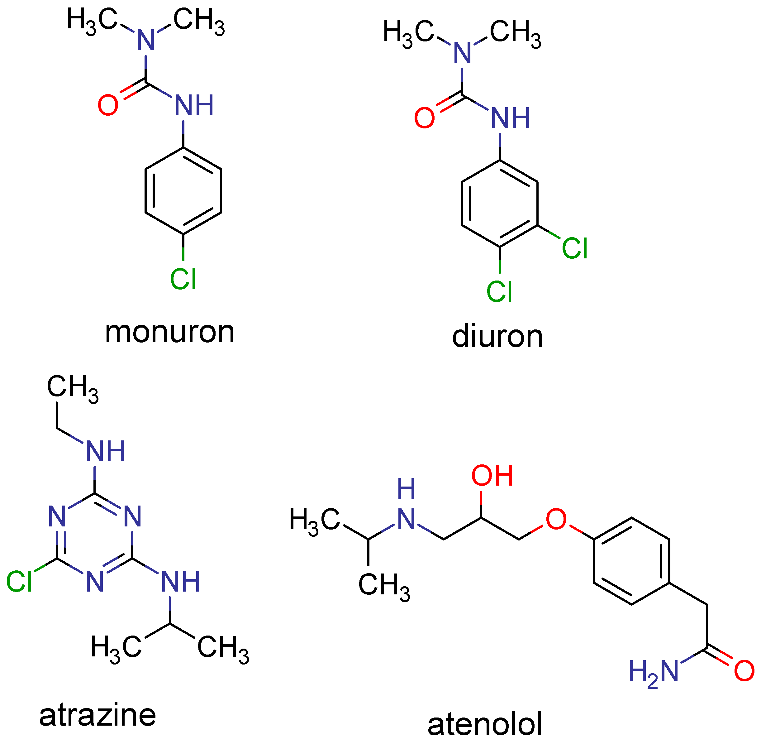
Predicting the Solubility of Nonelectrolyte Solids Using a Combination of Molecular Simulation with the Solubility Parameter Method MOSCED: Application to the Wastewater Contaminants Monuron, Diuron, Atrazine and Atenolol

Abstract

Methods to predict the equilibrium solubility of nonelectrolyte solids are indispensable for early-stage process development, design, and feasibility studies. Conventional analytic methods typically require reference data to regress parameters, which may not be available or limited for novel systems. Molecular simulation is a promising alternative, but is computationally intensive. Here, we demonstrate the ability to use a small number of molecular simulation free energy calculations to generate reference data to regress model parameters for the analytical MOSCED (modified separation of cohesive energy density) model. The result is an efficient analytical method to predict the equilibrium solubility of nonelectrolyte solids. The method is demonstrated for the wastewater contaminants monuron, diuron, atrazine and atenolol. Predictions for monuron, diuron and atrazine are in reasonable agreement with MOSCED parameters regressed using experimental solubility data. Predictions for atenolol are inferior, suggesting a potential limitation in the adopted molecular models, or the solvents selected to generate the necessary reference data.

1. Introduction

The ability to predict the equilibrium solubility of nonelectrolyte solids is important for a wide range of chemical, biological, and environmental processes. In the present study, we consider the environmental contaminants monuron, diuron, atrazine, and atenolol (see Figure 1). The herbicides monuron, diuron and atrazine make their way into surface- and ground-water sources typically as agricultural runoff. Although their toxicity is known, their low concentration makes removal and treatment problematic [1,2,3]. Atenolol is a commonly prescribed cardio-selective beta-blocker which is unable to be metabolized by the human body. Consequently, approximately half of the administered dose enters wastewater streams [4,5,6]. Conventional wastewater treatments plants are not designed to remove these contaminates as their concentration is typically considered low, and below toxic exposure levels. However, concerns exist over long-term exposure [5,7,8,9,10].

The development of novel processes to capture and remove contaminants from the environment is highly desirable. Central to the design of novel separations processes is the underlying phase equilibrium, here specifically the equilibrium solubility. Given the range of both potential contaminants and solvents, predictive methods are necessary. Given the importance of being able to predict the solubility of nonelectrolyte solids, considerable work has been done in this area. We can place this work in two camps. First are efficient analytic-based equations. Promising predictions have been made using the theoretically based NRTL-SAC model [11], MOSCED (modified separation of cohesive energy density) model [12], and the PC-SAFT equation of state [13,14]. However, reference data are first required to determine the necessary model parameters for the solute or mixing rules. Second is the use of molecular simulation [15,16,17,18]. With molecular simulation one may not only predict solubility devoid of reference data, but molecular simulation may additionally be used to probe the underlying intermolecular interactions. However, blind predictions using molecular simulation are computationally expensive and may not be feasible for design applications.

Recent efforts have been made to combine molecular simulation with the theoretically based, analytical, MOSCED model [19,20,21]. The result is a novel method combining the strength of both MOSCED and molecular simulation, while eliminating their shortcomings. Specifically, a limited number of molecular simulation solvation free energy calculations may be used to generate reference data from which MOSCED parameters may be regressed. Once MOSCED parameters are regressed, MOSCED may be used to efficiently make predictions in a range of solvents and over a range of temperatures. Moreover, previous work has suggested these predictions are improved as compared to using molecular simulation alone due to the implicit inclusion of reference data via the reference MOSCED parameters used during the regression.

The equilibrium solubility of a nonelectrolyte solid solute may be described by the classical equations of solid–liquid equilibrium. For the case of a solid solute (component 2) in a pure solvent (component 1) we have [22]:

$$ln{x}_2=-ln{\gamma }_{2,1}\left(T,P,x_2\right)+ln\frac{f_2^{\mathrm{S}}\left(T,P\right)}{f_2^0\left(T,P\right)}$$

(1)

where $x_2$ and ${\gamma }_{2,1}$ are the solute mole fraction and Lewis–Randall (or Raoult’s Law) normalized activity coefficient at equilibrium, T is the temperature, P is the pressure, and $f_2^{\mathrm{S}}$ and $f_2^0$ are the fugacity of the pure solid solute and pure subcooled liquid solute, respectively. The latter term is a property only of the pure solute, while the former term accounts for solute-solvent relative to solute-solute interactions. As a pure component property, the term $f_2^{\mathrm{S}}/f_2^0$ may readily be estimated using limited properties of the solute at the melting point [22,23,24,25,26] or may be predicted using molecular simulation so long as the solute solid crystal structure is known [15,16,17,18]. The focus in this work will therefore be on computing ${\gamma }_{2,1}$.

In the present study we will use the solubility parameter method MOSCED [12,19,20,21,27,28,29,30,31,32,33,34,35,36,37,38,39,40,41,42,43,44]. The use of solubility parameter-based methods is advantageous because they allow one to not only predict phase behavior using a simple analytic equation, but they can help offer an explanation in terms of the responsible molecular-level interactions. Analogous to UNIQUAC (universal quasichemical activity coefficient model), the limiting activity coefficient of component 2 in 1, ${\gamma }_{2,1}^{\infty }$, can be written as the sum of a combinatorial (COMB) and residual (RES) contribution [22,45]:

$$ln{\gamma }_{2,1}^{\infty }=ln{\gamma }_{2,1}^{\infty ,\mathrm{COMB}}+ln{\gamma }_{2,1}^{\infty ,\mathrm{RES}}$$

(2)

where COMB refers the entropic contribution which results from the size and shape dissimilarity of the components, and RES refers to the enthalpic contribution which results from intermolecular interactions. The advantage of MOSCED over similar solubility parameter-based methods is in its treatment of association interactions, allowing for both negative and positive values of $ln{\gamma }_{2,1}^{\infty ,\mathrm{RES}}$ in agreement with reality. Further discussion of MOSCED and the treatment of association interactions is provided in the supporting information accompanying the electronic version of this manuscript.

However, a shortcoming of MOSCED has always been a limitation of available parameters. Most recently, MOSCED was subject to a “revision” in 2005 [12] where parameters were regressed using reference limiting activity coefficients for 130 organic solvents, water, two room temperature ionic liquids (ILs), and five non-condensable gases. They additionally demonstrated the ability to obtain parameters for nonelectrolyte solids by fitting to experimental solubility data. However, for all these cases, experimental reference data are first needed for a compound of interest to regress parameters. For a novel compound, early in the design process, or for feasibility studies, such data are likely not available. As a result, recent efforts have been focused on developing techniques to predict MOSCED parameters devoid of experimental reference data. This work has included the use of molecular simulation [19,20,21], electronic structure calculations [20,21,37,38,39,42], and group contribution methods [35,37]. Here we demonstrate the use of molecular simulation to predict MOSCED parameters for the environmental contaminants: monuron, diuron, atrazine and atenolol. Parameters are regressed using reference data predicted using molecular simulation, and then used to predict solubility in a range of non-aqueous solvents. Using a relatively small number of molecular simulations we can parameterize MOSCED, allowing us to extrapolate to other solvents, solvent mixtures, and temperatures. The result is an efficient tool for early-stage process development and design applications. In support of this work, we have devolved an interactive MOSCED calculator capable of predicting limiting activity coefficients for a binary pair at a given temperature. (See Appendix A).

2. Method

2.1. MOSCED

Using MOSCED $ln{\gamma }_{2,1}^{\infty ,\mathrm{RES}}$ is calculated using the following system of equations [12,27]:

$$\begin{array}{c}ln{\gamma }_{2,1}^{\infty ,\mathrm{RES}}=\frac{v_2}{RT}\left[{\left({\lambda }_1-{\lambda }_2\right)}^2+\frac{q_1^2{q}_2^2{({\tau }_1^{\left(T\right)}-{\tau }_2^{\left(T\right)})}^2}{{\psi }_1}+\frac{({\alpha }_1^{\left(T\right)}-{\alpha }_2^{\left(T\right)})({\beta }_1^{\left(T\right)}-{\beta }_2^{\left(T\right)})}{{\xi }_1}\right]\\ {\alpha }_i^{\left(T\right)}={\alpha }_i{\left(\frac{293\mathrm{K}}{T}\right)}^{0.8},{\beta }_i^{\left(T\right)}={\beta }_i{\left(\frac{293\mathrm{K}}{T}\right)}^{0.8},{\tau }_i^{\left(T\right)}={\tau }_i{\left(\frac{293\mathrm{K}}{T}\right)}^{0.4}\\ {\psi }_1=\mathrm{POL}+0.002629{\alpha }_1^{\left(T\right)}{\beta }_1^{\left(T\right)}\\ {\xi }_1=0.68\left(\mathrm{POL}-1\right)+{\left[3.4-2.4exp\left(-0.002687{\left({\alpha }_1{\beta }_1\right)}^{1.5}\right)\right]}^{{\left(293\mathrm{K}/T\right)}^2}\\ \mathrm{POL}=q_1^4\left[1.15-1.15exp\left(-0.002337{\left({\tau }_1^{\left(T\right)}\right)}^3\right)\right]+1\end{array}$$

(3)

where R is the molar gas constant, T is the absolute temperature, $v_2$ is the (liquid) molar volume of the solute, ${\lambda }_i$, ${\tau }_i$, ${\alpha }_i$ and ${\beta }_i$ are the solubility parameters due to dispersion, polarity, and hydrogen bond acidity and basicity, respectively, and the induction parameter, $q_i$, reflects the ability of the nonpolar part of a molecule to interact with a polar part, where $i=\{1,2\}$. The terms ${\psi }_1$ and ${\xi }_1$ are (solvent dependent) asymmetry terms; these terms are not adjustable but are a function of the solvent solubility parameters. The superscript $\left(T\right)$ is used to indicate temperature dependent parameters, where the temperature dependence is computed using the empirical correlations provided in Equation (3) with a reference temperature of 293 K (20 °C). The combinatorial contribution is calculated using a modified Flory-Huggins equation [12,27]:

$$\begin{array}{c}ln{\gamma }_{2,1}^{\infty ,\mathrm{COMB}}=ln{\left(\frac{v_2}{v_1}\right)}^{a{a}_2}+1-{\left(\frac{v_2}{v_1}\right)}^{a{a}_2}\\ a{a}_2=0.953-0.002314\left[{\left({\tau }_2^{\left(T\right)}\right)}^2+{\alpha }_2^{\left(T\right)}{\beta }_2^{\left(T\right)}\right]\end{array}$$

(4)

where $v_1$ is the molar volume of the solvent, and $a{a}_2$ is an empirical (solute dependent) term to modify the size dissimilarity for polar and hydrogen bonding interactions. The term $a{a}_2$ is not adjustable, but is a function of the solubility parameters of the solute. For all cases $a{a}_2\le 0.953$, effectively reducing the size dissimilarity and magnitude of the combinatorial contribution, with the value smaller for polar and associating compounds. An equivalent expression for the residual and combinatorial contribution to the limiting activity coefficient for component 1 in 2 (${\gamma }_{1,2}^{\infty ,\mathrm{RES}}$ and ${\gamma }_{1,2}^{\infty ,\mathrm{COMB}}$) can be written by switching the subscript indices in Equations (3) and (4).

Using MOSCED we are restricted predicting limiting activity coefficient. Nonetheless, the predicted limiting activity coefficients can be used directly to obtain parameters for a binary interaction excess Gibbs free energy model, which in turn can be used to make composition dependent predictions [22,34,46,47]. Refs. [12,33] compared the use of Wilson’s equation and UNIQUAC with MOSCED to model the solubility of nonelectrolyte solids, and recommend the use of Wilson’s equation [22]. We will therefore adopt the use of Wilson’s equation in the present study. Further discussion of MOSCED and Wilson’s equation is provided in the supporting information accompanying the electronic version of this manuscript.

Molecular Simulation

In the present study, we will use molecular simulation to predict MOSCED parameters. In general, we will generate a set of reference data from which MOSCED parameters may be regressed. Using molecular simulation, we can calculate the solvation free energy of a solute (component i) at infinite dilution in a solvent (component j), $\Delta G_{i,j}^{\mathrm{solv}}$, where $i=${1 or 2} and $j=${1 or 2} [48]. The solvation free energy in this context is defined as taking a solute from a non-interacting ideal-gas state to solution at the same molecular density (or concentration). The solvation free energy is readily related to the limiting activity coefficient (${\gamma }_{i,j}^{\infty }$) as [19,49,50,51]:

$$ln{\gamma }_{i,j}^{\infty }\left(T,P\right)=\frac{1}{RT}\left[\Delta G_{i,j}^{\mathrm{solv}}\left(T,P\right)-\Delta G_{i,i}^{\mathrm{self}}\left(T,P\right)\right]+ln\frac{v_i\left(T,P\right)}{v_j\left(T,P\right)}$$

(5)

where $\Delta G_{i,i}^{\mathrm{self}}$ is the solute “self”-solvation free energy, and $v_i$ and $v_j$ correspond to the pure liquid molar volume of component i and j, respectively. The difference $\Delta G_{i,j}^{\mathrm{solv}}-\Delta G_{i,i}^{\mathrm{self}}$ is equivalent to the transfer free energy of i from a solution of pure i to pure j (in which it is infinitely dilute). When $i=j$ we obtain the correct limiting behavior that ${\gamma }_{i,i}^{\infty }=1$. The self-solvation free energy, $\Delta G_{i,i}^{\mathrm{self}}$, may be calculated by performing a solvation free energy calculation for component i in itself. Although such a calculation may readily be performed when component i is a liquid at the conditions of interest, in the present study we are interested in components which are solid at the conditions of interest for which we would have a subcooled liquid. Molecular simulation of a subcooled liquid should be avoided [52]. Nonetheless, we have proposed several schemes to overcome this limitation.

First, we can relate $\Delta G_{i,i}^{\mathrm{self}}$ to the pure liquid fugacity of component i, $f_i^0$, as [52]:

$$ln{f}_i^0\left(T,P\right)=\frac{1}{RT}\Delta G_{i,i}^{\mathrm{self}}\left(T,P\right)+ln\frac{RT}{v_i\left(T,P\right)}$$

(6)

We can expand $f_i^0$ as [22]:

$$f_i^0\left(T,P\right)={\varphi }_i^{\mathrm{sat}}\left(T\right)P_i^{\mathrm{sat}}\left(T\right)exp\left\{{\int }_{P^{\mathrm{sat}}}^P\frac{v_i\left(T,P\right)}{RT}dP\right\}$$

(7)

where ${\varphi }_i^{\mathrm{sat}}$ and $P_i^{\mathrm{sat}}$ are the fugacity coefficient and vapor pressure of pure component i at saturation at T, and the term in brackets is the Poynting correction, and accounts for the change in fugacity in going from $P^{\mathrm{sat}}$ to P at constant T. If we assume that the vapor phase is an ideal gas and that the Poynting correction is negligible, we have [22,52,53,54]:

$$ln{f}_i^0\left(T,P\right)=ln{P}_i^{\mathrm{sat}}\left(T\right)=\frac{1}{RT}\Delta G_{i,i}^{\mathrm{self}}\left(T,P\right)+ln\frac{RT}{v_i\left(T,P\right)}$$

(8)

If we are at low pressures well removed from the critical point, and we have a non-self-associating fluid (i.e., no carboxylic acid), use of this expression is generally reasonable. The significance of this expression is that from the Clapeyron equation we expect $ln{f}_i^0$ to scale linearly with respect to $1/T$ [22]. This presents a means by which molecular simulations may be used to compute $\Delta G_{i,i}^{\mathrm{self}}$ and $v_i$ at elevated temperatures where the component exists as a liquid, and then extrapolate to the conditions of interest below the melting point. Additionally, from these simulations at elevated temperatures one can extrapolated the computed liquid molar volume to 293 K to obtain MOSCED parameter $v_2$.

Although it is possible to obtain $f_i^0$ from molecular simulation, alternatively one might attempt to use reference data (via $P_i^{\mathrm{sat}}$). However, it is important that the quantities of interest be computed in a consistent fashion [49]. Although not used in the present study, if the calculation of $f_i^0$ is not possible or undesirable, in our previous work we have proposed two related schemes which are described in the Appendix B.

2.2. $f_2^{\mathrm{S}}/f_2^0$

The solubility of a nonelectrolyte solid solute (component 2) in a pure solvent (component 1) is given by Equation (1). The latter term is a property only of the pure solute, while the former term (${\gamma }_{2,1}$) accounts for solute-solvent relative to solute-solute interactions. The focus of the present study is on the calculation of the term ${\gamma }_{2,1}$. The pure component property $f_2^{\mathrm{S}}/f_2^0$ necessary to compute the equilibrium solubility via Equation (1) is therefore computed using experimental data and the method of Nordström and Rasmuson [25]. In summary, assuming there are no solid/solid phase transitions between the melting point and the conditions of interest we have [22,23,24,25,26]:

$$ln\frac{f_2^{\mathrm{S}}\left(T,p\right)}{f_2^0\left(T,p\right)}=-\Delta G_2^m\left(T,p\right)=\frac{\Delta H_2^m\left(T_2^m\right)}{R}\left[\frac{1}{T_2^m}-\frac{1}{T}\right]-\frac{1}{RT}{\int }_{T_2^m}^T\Delta C_{p,2}dT+\frac{1}{R}{\int }_{T_2^m}^T\frac{\Delta C_{p,2}}{T}dT$$

(9)

where $\Delta G_2^m$ is the molar Gibbs free energy of melting (or fusion), $T_2^m$ is the normal melting point temperature, and $\Delta H_2^m$ is the molar enthalpy of melting (or fusion) at $T_2^m$. $\Delta C_{p,2}$ is the difference in the isobaric heat capacity between the liquid and solid solute. Accurately determining $\Delta C_{p,2}$ is challenging because it involves a subcooled liquid phase below the melting point. A common approximation is to assume [25]:

$$\Delta C_{p,2}=\sigma \frac{\Delta H_2^m\left(T_2^m\right)}{T_2^m}$$

(10)

where $\sigma$ is a constant. When $\sigma =0$ we recover the common engineering assumption that $\Delta C_{p,2}=0$ and the enthalpy of fusion is constant and equal to its value at the melting point [22]. When $\sigma =1$ we recover the assumption that $\Delta C_{p,2}$ is constant and equal to the molar entropy of melting (or fusion) at the melting point [23], $\Delta S_2^m=\Delta H_2^m\left(T_2^m\right)/T_2^m$. Recently, Nordström and Rasmuson [25] took $\sigma$ to be an adjustable parameter and optimized its value at 10, 15, 20, 25 and 30 °C using temperature dependent equilibrium solubility data for solutes of a range of chemical complexities. Taking $\Delta C_{p,2}$ to be constant and given by Equation (10), we obtain:

$$ln\frac{f_2^{\mathrm{S}}\left(T,p\right)}{f_2^0\left(T,p\right)}=\frac{\Delta H_2^m\left(T_2^m\right)}{R{T}_2^m}\left[\left(1-\frac{T_2^m}{T}\right)\left(1-\sigma \right)+\sigma ln\frac{T_2^m}{T}\right]$$

(11)

The reference value of $\sigma$ at 10, 15, 20, 25 and 30 °C is 1.958, 1.940, 1.922, 1.897 and 1.868, respectively [25]. Although here we will adopt experimental values of $\Delta H_2^m$ and $T_2^m$, their values could readily be predicted using group contribution methods or other means [15,16,17,18,55].

3. Computational Details

3.1. Molecular Simulation

Interactions were modeled using a “class I” potential energy function where all non-bonded intermolecular interactions were accounted for using a combined Lennard-Jones (LJ) plus fixed-point charge model [56,57]. The solvents studied were: n-hexane, 2,5-dimethylhexane, 1-hexene, 1-octene, methanol, ethanol, 1-propanol, 2-propanol, diethylether, acetone, butanone, benzene and water. Benzene was modeled using the Explicit Hydrogen Transferable Potentials for Phase Equilibria (TraPPE-EH) force field [58] and all other organic solvents were modeled with the United Atom TraPPE (TraPPE-UA) force field [59,60,61,62,63,64]. Here benzene (and aromatic rings in general) is modeled using TraPPE-EH, and TraPPE-UA is used in all other cases. Although a 6-site TraPPE-UA model exists for benzene, the 12-site TraPPE-EH model has been shown to more accurately represent benzene dimer energetics which we expect to be important for accurately modeling solvation [58,61]. Although in the original TraPPE-EH work, benzene is modeled as completely rigid, here we adopt angle-bending and dihedral parameters from the General AMBER Force Field (GAFF) [65,66]. Additionally, while TraPPE-UA and TraPPE-EH treat bonds as rigid, here we will only constrain bonds involving hydrogens; missing bond stretching parameters were taken from the united atom force field file gmx.ff in GROMACS 4.6.3 [67,68,69] for use with TraPPE-UA, and from GAFF for benzene. Water was modeled with TIP4P [70], which has been shown to work well with TraPPE force field models [71,72]. This is exactly the same set of solvent models used in our previous work [20].

The force fields for monuron, diuron, atrazine and atenolol (the studied solutes) were all constructed based on the TraPPE-EH force field [58,62,63,64,73,74], and follow our previous work [20,52,75]. Partial atomic charges for the solutes were obtained in a similar fashion as the original TraPPE-EH parameterization [58,73,74] and follow our previous work [75]. First, the gas-phase structure for each solute was optimized at the M06-2X/cc-pVTZ level of theory/basis set [76,77]. Second, a single point energy calculation was performed on the gas-phase optimized structure at the M06-2X/6-31G(d) level of theory/basis set [76,77] in the SM8 universal solvation model for 1-octanol [78]. Partial atomic charges were computed using the CM4 charge model [79,80] obtained during the single point energy calculation in SM8 1-octanol. TraPPE-EH adopted 1-octanol as the reference solvent for determining partial charges as it possesses both polar and nonpolar character [58]. All the electronic structure calculations were performed using QChem 4.0.1 [81]. The force field for atrazine and atenolol are the same as in our previous work [75].

For the case of monuron and diuron, we additionally investigated the use of a second, similar set of partial atomic charges. Again, we first performed a gas-phase optimization for the solute at the M06-2X/cc-pVTZ level of theory/basis set. Second, a single point energy calculation was performed on the gas-phase optimized structure at the M06-2X/6-31G(d) level of theory/basis set in the SMD universal solvation model for 1-octanol [82]. All the electronic structure calculations were performed using Gaussian 09 [83]. Third, partial atomic charges were then obtained from the electrostatic potential (obtained in step 2) using the restrained electrostatic potential (RESP) [84,85] method in ANTECHAMBER (part of the AMBER 12 simulation suite) [66,86,87].

We emphasize that in the original TraPPE-EH work for aromatics [58,73,74] partial charges were obtained using CM4 charges with the SM8 universal solvation model for 1-octanol. Here the motivation for the additional use of SMD is two-fold. First, to assess the sensitivity of the results on the charge parameterization method, where here we anticipate that the behavior of SMD will be similar SM8. Second, and closely related, the SM8 universal solvation model may not be available in the software accessible to an interested user [88]. This is demonstrated here only for monuron and diuron because of the availability of reference solubility data in a much larger number of unique solvents. Additional continuum solvent models and charge parameterization methods are available [89]. However, a thorough evaluation is beyond the scope of the present study.

All the intramolecular parameters for the solutes were taken from the General Amber Force Field (GAFF) [65]. Parameters were generated using ANTECHAMBER and converted from AMBER to GROMACS format using ACPYPE [90,91]. Throughout the present study, all solute bonds involving hydrogens were held fixed.

The present study requires the calculation of configurational properties, allowing one to use either Monte Carlo or molecular dynamics (MD) simulations to sample configurational phase space. Here we used MD and performed all calculations with GROMACS 4.6.3, following the procedure used in our previous work [20]. Solvation free energies were computed using the multi-state Bennett’s acceptance ratio method (MBAR) [92], using the soft-core potential method to couple/decouple intermolecular LJ interactions [93,94]. The GROMACS trajectory files were analyzed using the script distributed with the Python implementation of MBAR (PyMBAR) [95,96,97].

All the GROMACS force field files used in the present study along with additional discussion of the solute force fields are provided as supporting information accompanying the electronic version of this manuscript. A detailed discussion of the simulation procedure and details may be found in the supporting information accompanying the electronic version of our previous work [20].

3.2. Regressing MOSCED Parameters

Using molecular simulation, for each solute the infinite dilution activity coefficient (${\gamma }_{2,1}^{\infty }$) was computed in 13 different solvents (n-hexane, 2,5-dimethylhexane, 1-hexene, 1-octene, methanol, ethanol, 1-propanol, 2-propanol, diethylether, acetone, butanone, benzene and water) at 298.15 K, by means of Equations (5) and (8). The solvents were chosen because both MOSCED and force field parameters were available, and they offered a variety of chemical functionalities. MOSCED parameters were obtained by minimizing the objective function (OBJ)

$$\mathrm{OBJ}=\sum _{i=1}^{N=13}{\left(ln{\gamma }_{2,i}^{\infty ,\mathrm{sim}}-ln{\gamma }_{2,i}^{\infty ,\mathrm{MOSCED}}\right)}^2$$

(12)

the squared difference between $ln{\gamma }_{2,i}^{\infty }$ computed using molecular simulation (“sim”) and using MOSCED (Equations (3) and (4)), as indicated by the superscript, where the summation is over all $N=13$ solvents. Log terms are used as it is the log value that is directly related to the solvation free energy which is computed (see Equation (5)). The optimization was performed using the differential evolution method [98] as implemented in GNU Octave [99]. Only values of the ${\lambda }_2$, ${\tau }_2$, ${\alpha }_2$ and ${\beta }_2$ solute MOSCED parameters were made adjustable; $v_2$ was fixed as the solute liquid molar volume at 293 K estimated by extrapolating liquid molar volumes computed at elevated temperatures and $q_2$ was set to 0.9 as suggested in ref. [12] for aromatic centered solutes. The differential evolution method is a global optimization technique and does not require or use initial estimates of the parameters. We specify only that the parameters are bound between 0 and 100 to limit the search. The differential evolution method was used here because it is a global method that has demonstrated good performance for a wide range of non-linear problems.

4. Results and Discussion

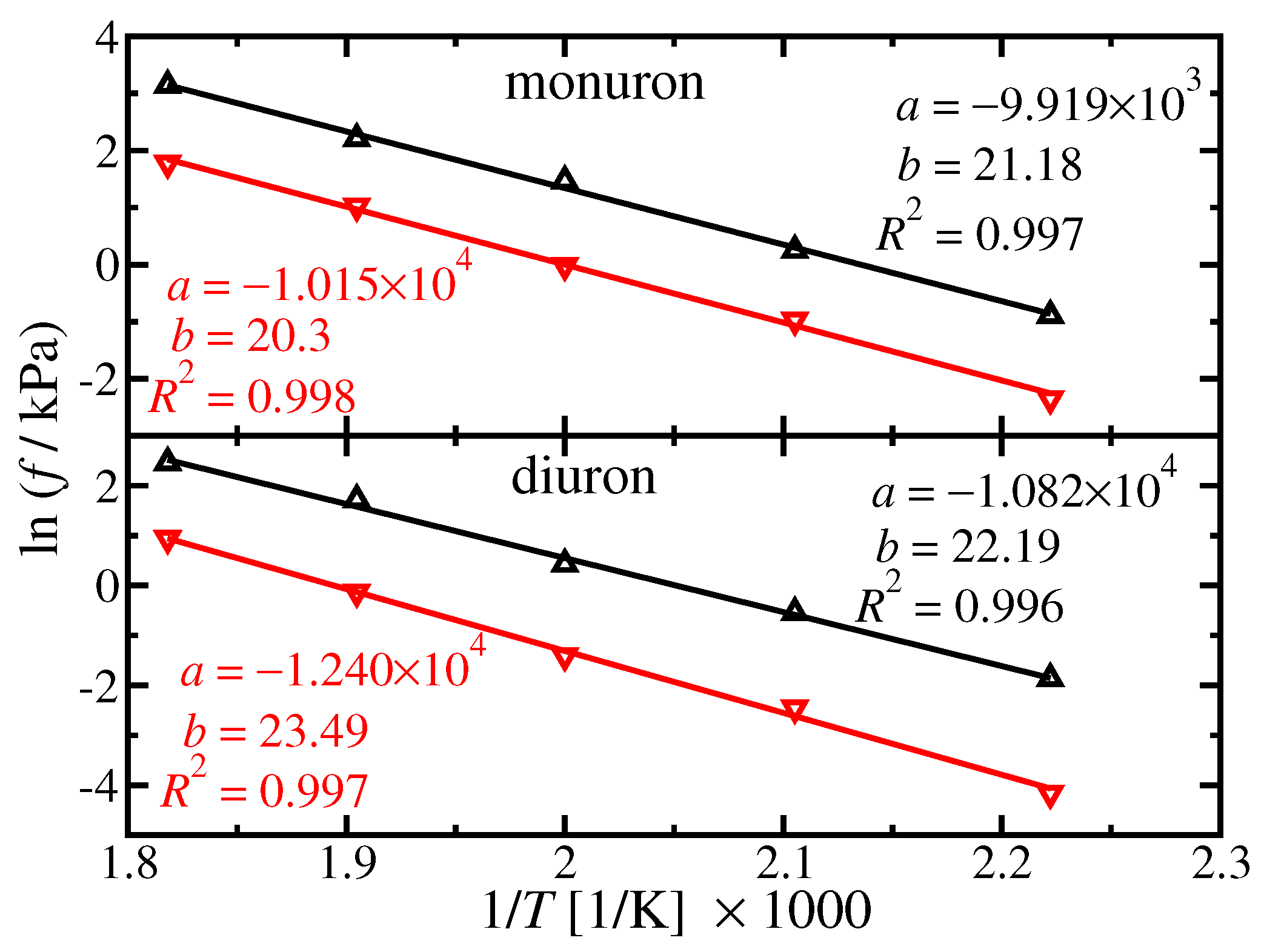
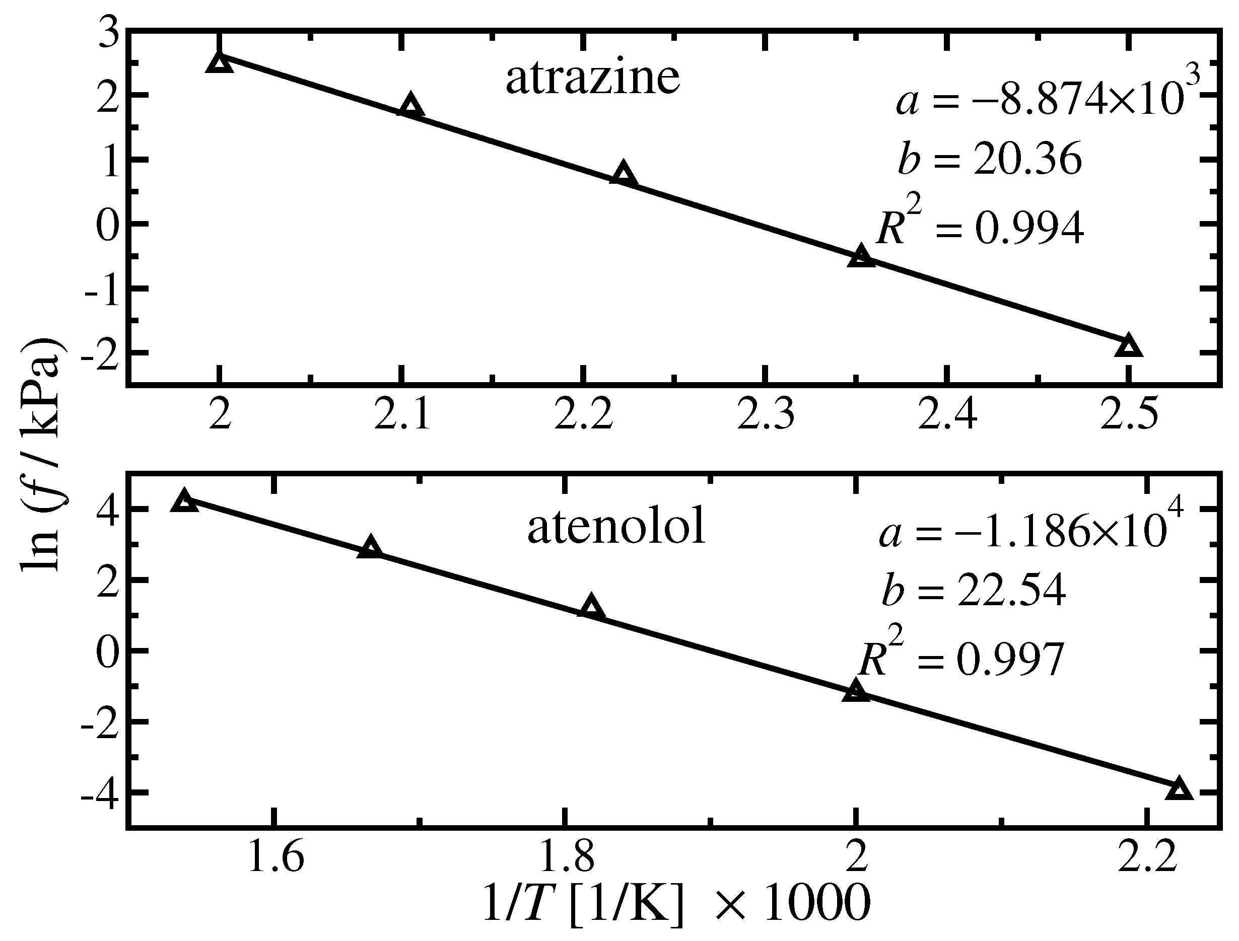
4.1. Pure Component Fugacity

The results of the pure component fugacity calculations using molecular simulation are shown in Figure 2 for the monuron and diuron and in Figure 3 for atrazine and atenolol. The solutes are all solid at ambient conditions. Calculations were therefore performed at elevated temperatures greater than the experimental normal melting point, and extrapolated to 298.15 K. Although simulations of the subcooled liquid may be performed, caution must be exercised as they may yield erroneous results [52]. All the computed fugacities were on the order of 10 kPa or less, where we expect $f^0\approx P^{\mathrm{sat}}$. As a result, $f^0$ was fit to and extrapolated using a Clausius-Clapeyron equation of the form $ln{f}_2^0=-a{T}^{-1}+b$, where a and b are constants, and the inverse of the uncertainty of $ln{f}^0$ was used to weight each datum during the regression. In all cases the fit was excellent, with coefficients of determination close to unity. The results are all tabulated in the supporting information accompanying the electronic version of this manuscript.

For monuron, diuron, atrazine, and atenolol, partial charges were obtained using the CM4 charge model in SM8 1-octanol. For the case of monuron and diuron, we additional used RESP charges in SMD 1-octanol. As seen in Figure 2, we observe a noticeable difference in the pure component fugacity when using the two charge models. The difference in general is on the order of one log unit. This result is not surprising and similar to the variability in hydration free energy with various partial charge parameterization schemes [89].

Likewise, the liquid molar volume was extrapolated to 293 K to obtain MOSCED parameter $v_2$ using the expression $lnv=aT+b$, where a and b are constants and the inverse of the uncertainty of $lnv$ was used to weight each datum during the regression. In all cases the fit was again excellent, and we obtain a coefficient of determination close to unity. The results are all tabulated in the supporting information accompanying the electronic version of this manuscript.

4.2. MOSCED Parameters

The MOSCED parameters regressed using a limited number of molecular simulation free energy calculations at 298.15 K are tabulated in

Table 1. The MOSCED parameters for the studied solutes obtained using reference data generated using molecular simulation free energy calculations at 298.15 K. For all cases we consider partial atomic charges obtained using the SM8 solvation model. For monuron and diuron we additionally considered partial atomic charges obtained using the SMD solvation model, and we list MOSCED parameters regressed in ref. [12] obtained from experimental solubility data (ref). $v_2$ has units of cm³/mol, and ${\lambda }_2$, ${\tau }_2$, ${\alpha }_2$, and ${\beta }_2$ all have units of (J/cm³)${}^{1/2}$. For all the solutes, $q_2=0.9$. N corresponds to the number of reference data used to regress the parameters, and $R^2$, RMSE, and AAPD are the resulting coefficient of determination, root mean squared error, and average absolute percent deviation, respectively. The statistics for the reference parameters for monuron and diuron were taken from ref. [12].

Solute	Method	${\mathit{v}}_2$	${\mathit{\lambda }}_2$	${\mathit{\tau }}_2$	${\mathit{\alpha }}_2$	${\mathit{\beta }}_2$	N	${\mathit{R}}^2$	RMSE	AAPD
monuron	ref	152.80	16.44	5.48	7.16	9.65	32			22.0
	SM8	164.75	15.65	1.38	13.11	7.42	13	0.985	0.430	34.5
	SMD	162.98	12.49	0.00	18.63	6.87	13	0.931	1.233	156.7
diuron	ref	164.80	16.99	4.12	7.88	9.88	37			36.3
	SM8	176.94	17.07	3.00	12.37	8.26	13	0.900	1.282	98.0
	SMD	176.32	17.14	2.72	14.91	9.83	13	0.984	0.607	56.6
atrazine	SM8	183.35	15.32	3.04	9.89	4.26	13	0.984	0.438	38.1
atenolol	SM8	253.43	14.20	1.53	12.18	4.03	13	0.953	1.116	191.5

for monuron, diuron, atrazine and atenolol. For all cases we consider partial atomic charges obtained using the SM8 solvation model. For monuron and diuron we additionally considered partial atomic charges obtained using the SMD solvation model, and we list MOSCED parameters regressed in ref. [12] obtained from experimental solubility data.

First, let us consider the case of monuron and diuron. For the case of monuron, we find that the calculations with the SM8 partial charges result in both the greatest agreement with the set of reference parameters, and are better correlated by MOSCED as compared to the calculations with the SMD partial charges. For diuron, except for ${\beta }_2$, the calculations with the SM8 partial charges again result in the greatest agreement with the set of reference parameters. Nonetheless, while SMD is in better agreement with the reference value of ${\beta }_2$, SM8 is in better agreement with the self-association term ${\alpha }_2{\beta }_2$. On the other hand, we find that the calculations with the SMD partial charges are better correlated by MOSCED. We emphasize that here we are using MOSCED to correlate predicted data, which will exhibit deviations from experiment [49,78,82]. Previously, we have found when training MOSCED with predicted data that the predictions ultimately made with the trained MOSCED model are superior to predictions made with the method used to generate the training data alone. We believe this results from the implicit inclusion of the experimental data used to train the original MOSCED model, and the resulting solvent parameters used here [19,20,21,38]. For both monuron and diuron, the reference parameters have ${\beta }_2>{\alpha }_2$ indicating that monuron and diuron are both stronger proton acceptors than donors. However, with the predicted values we have ${\alpha }_2>{\beta }_2$ suggesting they are stronger proton donors than acceptors, and further the difference is much larger.

In

Table 2. The computed dimensionless solvation free energy, $\Delta G_{i,j}^{\mathrm{solv}}/\left(RT\right)$, for solute i in solvent j at 298.15 K. For all cases we consider partial atomic charges obtained using the SM8 solvation model. For monuron and diuron we additionally considered partial atomic charges obtained using the SMD solvation model. The subscripts correspond to the uncertainty in the last two decimal places.

	Monuron		Diuron		Atrazine	Atenolol
Solvent	SM8	SMD	SM8	SMD	SM8	SM8
n-hexane	$-{15.31}_{07}$	$-{15.55}_{08}$	$-{16.82}_{07}$	$-{16.91}_{07}$	$-{15.62}_{07}$	$-{22.08}_{05}$
2,5-dimethylhexane	$-{16.72}_{11}$	$-{16.91}_{11}$	$-{18.18}_{12}$	$-{18.38}_{12}$	$-{16.52}_{11}$	$-{23.70}_{07}$
1-hexene	$-{15.33}_{07}$	$-{15.63}_{07}$	$-{16.77}_{07}$	$-{16.96}_{07}$	$-{15.64}_{07}$	$-{22.09}_{05}$
1-octene	$-{15.27}_{08}$	$-{15.34}_{08}$	$-{16.68}_{08}$	$-{16.82}_{09}$	$-{15.64}_{08}$	$-{22.09}_{06}$
benzene	$-{18.38}_{09}$	$-{14.49}_{09}$	$-{20.16}_{11}$	$-{21.26}_{10}$	$-{18.83}_{09}$	$-{26.39}_{06}$
methanol	$-{22.95}_{07}$	$-{26.63}_{07}$	$-{24.40}_{08}$	$-{28.63}_{08}$	$-{20.78}_{07}$	$-{30.62}_{05}$
ethanol	$-{23.20}_{08}$	$-{26.03}_{09}$	$-{24.59}_{10}$	$-{28.57}_{10}$	$-{20.27}_{08}$	$-{30.22}_{06}$
1-propanol	$-{22.80}_{09}$	$-{26.03}_{10}$	$-{24.28}_{12}$	$-{28.05}_{12}$	$-{19.78}_{09}$	$-{30.05}_{07}$
2-propanol	$-{22.50}_{11}$	$-{25.30}_{12}$	$-{23.62}_{12}$	$-{27.45}_{11}$	$-{19.42}_{10}$	$-{29.22}_{08}$
acetone	$-{23.19}_{07}$	$-{25.00}_{07}$	$-{24.80}_{07}$	$-{27.77}_{07}$	$-{22.22}_{07}$	$-{31.42}_{04}$
butanone	$-{22.75}_{07}$	$-{24.55}_{07}$	$-{24.27}_{08}$	$-{26.98}_{08}$	$-{21.91}_{07}$	$-{30.69}_{05}$
diethylether	$-{21.31}_{06}$	$-{22.87}_{06}$	$-{22.68}_{06}$	$-{25.23}_{06}$	$-{21.15}_{06}$	$-{29.62}_{04}$
water	$-{14.53}_{11}$	$-{19.38}_{12}$	$-{14.82}_{13}$	$-{19.36}_{14}$	$-{10.41}_{13}$	$-{16.48}_{05}$

we tabulate the computed dimensionless solvation free energies. For monuron and diuron, the choice of partial charges noticeably effects the solvation free energy in benzene, alcohols, ketones, diethylether, and water. We emphasize that in comparing SM8 and SMD, the only difference is in the resulting partial charges of the solute. Additionally, the TraPPE-UA models for n-hexane, 2,5-dimethylhexane, 1-hexene, and 1-octene do not include the use of partial charges [59,60,61]. For this reason, the difference between SM8 and SMD in the alkanes and alkenes is minor, and the effect is greatest in solvents where we expect association (hydrogen bonding) to be important. Except for benzene, the solvation free energies using SMD partial charges are all lower (more negative) as compared to SM8. This is indicative of an increased affinity for the solvent relative to a non-interacting ideal-gas state. The same was true when computing the pure component fugacity; we found that with the SMD partial charges the self-solvation free energy was lower (or more negative) as compared to SM8. This underlines the importance of computing the solvation free energy and self-solvation free energy in a consistent fashion [49], and the results are sensitive to the force field and the associated partial charges.

For atrazine and atenolol, the ability of MOSCED to correlate the predicted limiting activity coefficients is very good, and comparable to the best fits for monuron and diuron. Moreover, the parameters appear reasonable. The force fields for atrazine and atenolol were adopted from our recent molecular simulation study of the compounds in 1-n-butyl-3-methylimidazolium-based ionic liquids for potential wastewater treatment applications [75]. In that work we found that the solutes had a large affinity for 1-n-butyl-3-methylimidazolium acetate. This resulted from strong hydrogen bonding between the solute and acetate anion, where the solute was the hydrogen bond donor and acetate was the hydrogen bond acceptor. Moreover, we found that atenolol was the stronger hydrogen bond donor, which is consistent with our results here where ${\alpha }_2$ for atenolol is greater than for atrazine.

4.3. Solubility Predictions

Solubility predictions are made via Equation (1). MOSCED is used to predict ${\gamma }_{1,2}^{\infty }$ and ${\gamma }_{2,1}^{\infty }$, which may then be used to parameterize Wilson’s equation to compute ${\gamma }_{2,1}$. Although the focus here is on MOSCED and predicting limiting activity coefficients, for the nonelectrolyte solids studied here only experimental solubility data are available for comparison. For solubility prediction, an estimate of the pure component term $f_2^{\mathrm{S}}/f_2^0$ is necessary, which we compute here using Equation (11). In the present study, we used a piecewise cubic Hermite interpolating polynomial (pchip) as implemented in the function interp1 within GNU Octave [99] to compute $\sigma$ at a specific temperature over the range 10–30 °C. We will refer to this value of $\sigma$ as “opt” (optimal). We additionally make comparison to the common approximations of $\sigma =$0 and 1. The resulting solubility predictions in non-aqueous organic solvents are summarized in

Table 3. A summary of the predicted solubility ($x_2$) in non-aqueous solvents. For all cases we consider partial atomic charges obtained using the SM8 solvation model. For monuron and diuron we additionally considered partial atomic charges obtained using the SMD solvation model, and we list the results using MOSCED parameters regressed in ref. [12] using experimental solubility data (ref). N systems and N solvents corresponds to the number of systems and solvents, respectively, and AAPD and RMSE are resulting average absolute percent deviation and root mean squared error, respectively. $R^2$ and slope are the resulting coefficient of determination and slope of the corresponding parity plot. Please note that N systems ≥ N solvents because of the possibility of multiple temperatures.

					${\mathit{x}}_2$		$ln{\mathit{x}}_2$
Solute	N Systems	N Solvents	Method	$\mathit{\sigma }$	AAPD	RMSE$\times {10}^2$	RMSE	${\mathit{R}}^2$	Slope
monuron	32	31	ref	0	21.97	0.26	0.53	0.94	0.93
				1	110.15	0.91	0.81	0.94	0.93
				opt	325.15	2.68	1.44	0.95	0.94
			SM8	0	95.83	1.29	1.30	0.82	1.17
				1	190.63	3.01	1.29	0.82	1.16
				opt	401.98	5.86	1.59	0.83	1.14
			SMD	0	125.15	1.56	2.96	0.73	1.59
				1	227.99	3.38	2.60	0.73	1.58
				opt	404.31	6.30	2.39	0.74	1.56
diuron	36	36	ref	0	35.94	0.35	0.59	0.95	0.95
				1	98.80	0.70	0.73	0.95	0.95
				opt	281.92	1.97	1.32	0.95	0.95
			SM8	0	74.02	0.59	1.50	0.91	1.27
				1	120.38	1.54	1.15	0.92	1.27
				opt	218.97	3.24	1.19	0.92	1.26
			SMD	0	76.75	0.40	3.48	0.88	1.70
				1	114.17	0.93	2.95	0.88	1.70
				opt	196.85	2.36	2.55	0.88	1.70
atrazine	63	6	SM8	0	64.79	1.02	0.53	0.93	1.06
				1	277.12	2.65	1.32	0.91	0.79
				opt	720.13	5.05	2.04	0.75	0.47
atenolol	54	6	SM8	0	6506.42	8.92	3.02	0.69	0.58
				1	11,513.77	11.51	3.39	0.73	0.55
				opt	19,679.49	14.49	3.73	0.76	0.52

, and the predictions are tabulated in the supporting information accompanying the electronic version of this manuscript.

For monuron, the non-aqueous experimental solubility data used for comparison is all the single component solubility data available in Part 1 and 2 of DECHEMA’s “Solubility and Related Properties of Large Complex Chemicals” [100,101] for which MOSCED solvent parameters exist. This resulted in 32 reference solubilities in 31 unique solvents. The data from Part 1 was all at 298 K, and the data from Part 2 was all at 298.15 K [100,101]. The pure component values of $T_{m,2}$ and $\Delta H_2^{\mathrm{fus}}$ for monuron were taken from Part 1.

For diuron, the non-aqueous experimental solubility data used for comparison is all the single component solubility data available in Part 1 of DECHEMA’s “Solubility and Related Properties of Large Complex Chemicals” [100] for which MOSCED solvent parameters exist. This resulted in 36 reference solubilities in 36 unique solvents. The experimental data were all at 298.15 K. The pure component values of $T_{m,2}$ and $\Delta H_2^{\mathrm{fus}}$ were also taken from Part 1.

For atrazine, the non-aqueous experimental solubility data used for comparison is all from Jia et al. [102]. Data are available for atrazine in methanol, ethanol, 1-propanol, 2-propanol, 1-butanol, and ethyl acetate over the range 283.15–343.15 K. The pure component values of $T_{m,2}$ and $\Delta H_2^{\mathrm{fus}}$ were taken from Donnelly et al. [103].

For atenolol, the non-aqueous experimental solubility data used for comparison is all the single component solubility data available from refs. [104,105,106] for which MOSCED solvent parameters exist. This resulted in 54 reference solubilities in six unique solvents. The solvents are: ethanol, 1-octanol, 1,4-dioxane, dichloromethane, ethyl acetate, and n-hexane. The pure component values of $T_{m,2}$ and $\Delta H_2^{\mathrm{fus}}$ were taken from ref. [106].

First, let us consider the case of monuron and diuron. For these cases we make predictions using MOSCED parameters regressed in ref. [12] using experimental solubility data (ref). Having been regressed directly using experimental solubility data, we take this to be a limit on the level of accuracy we can achieve. For both monuron and diuron, the best set of predictions is made using $\sigma =0$. With our predicted MOSCED parameters, for both cases the best predictions are made using parameters regressed using SM8 partial charges and likewise with $\sigma =0$. The results for monuron and diuron are similar. Although when using the reference set of MOSCED parameters, our error in $x_2$ is on the order of $1\times {10}^{-3}$ mole fracs, with our predicted MOSCED parameters the errors are on the order of $1\times {10}^{-2}$ and $1\times {10}^{-3}$ mole fracs for monuron and diuron, respectively. To give perspective, for monuron the experimental reference values of $x_2$ span the range $5.09\times {10}^{-5}$ to $2.64\times {10}^{-2}$ mole fracs, with an average value of $6.83\times {10}^{-3}$ mole fracs. The only solvent for which reference data are available in Part 1 (at 298 K) and Part 2 (at 298.15 K) is ethyl acetate, with values of $9.96\times {10}^{-3}$ and $1.01\times {10}^{-2}$ mole fracs, respectively, for a difference of $1.14\times {10}^{-4}$. Similar for diuron the experimental reference values of $x_2$ span the range $1.83\times {10}^{-5}$ to $3.06\times {10}^{-2}$ mole fracs, with an average value of $5.42\times {10}^{-3}$ mole fracs. Although the agreement is not perfect, we emphasize the efficiency of the proposed method. Conventional solvation free energy calculations were performed for the solvent in 13 unique solvents, all at 298.15 K. This limited set of data was used to parameterized MOSCED, which allows extrapolation to additional solvents and temperatures. In fact, we can make predictions in any solvent for which MOSCED parameters exists; predictions were made in 31 unique solvents for monuron and 36 unique solvents for diuron. We would expect that the accuracy can be improved with additional optimization of the force fields and solvents used here, but this is beyond the scope of the present work. Here we demonstrate the sensitivity of the predictions on the solute partial charges adopted. Moreover, the accuracy of the predictions parameterized using molecular simulation generated data is not unreasonable as compared to the set of reference predictions (ref).

The results for atrazine are consistent with monuron and diuron. The results using SM8 partial charges and $\sigma =0$ are the top performer, and are the best of all the predictions made. The error in $x_2$ is on the order of $1\times {10}^{-2}$ mole fracs, and for $ln{x}_2$ we obtain both an $R^2$ and slope close to unity. As compared to monuron and diuron, reference solubility data is available only in six unique solvents: methanol, ethanol, 1-propanol, 2-propanol, 1-butanol and ethyl acetate. Although this does not represent a diverse set of solvents, it does span a range of temperatures from 283.15 K to 343.15 K. We emphasize that despite only performing solvation free energy calculations for atrazine in 13 solvents at 298.15 K, here we can make predictions over a range of temperatures. The experimental reference values of $x_2$ span the range $1.64\times {10}^{-3}$ to $5.42\times {10}^{-2}$ mole fracs, with an average value of $1.02\times {10}^{-2}$ mole fracs. Interestingly, despite the larger minimum value (and hence smaller range) as compared to monuron and diuron, the predictions exhibit a similar accuracy.

Finally, let us consider the case of atenolol. The best set of predictions again corresponds to $\sigma =0$. Although the error in $x_2$ is again on the order of $1\times {10}^{-2}$ mole fracs, the predictions are inferior to that of the other solutes. Please note that the very large value of AAPD is the result of the predictions in hexane; the experimental reference values are on the order of $1\times {10}^{-7}$ mole fracs while the predictions are on the order of $1\times {10}^{-4}$ to $1\times {10}^{-5}$ mole fracs. The cause for the inferior performance is unclear. Based on the structure of atenolol, we expect that will have a greater conformational dependence as compared to the other solutes, and therefore may be a limitation in the molecular models used.

5. Summary and Conclusions

The ability to model the underlying phase equilibrium is crucial for the design of novel separation processes. For early-stage process development, design, and feasibility studies, or for processes involving novel components, predictive methods are required. In the present study we are concerned with the ability to predict the equilibrium solubility of nonelectrolyte solids. Specifically, we consider the wastewater contaminants: monuron, diuron, atrazine, and atenolol. Given the importance of being able to predict the equilibrium solubility of nonelectrolyte solids, significant work has been done in this area.

Most common for design applications is the use of efficient analytic models. However, their use may be limited for novel systems as they typically first require reference data to determine the necessary model parameters for the solute or mixing rules. Recently, promising predictions have been made using molecular simulation. However, the use of molecular simulation is computationally expensive and may not be suitable for design applications. In the present study we demonstrated the ability to marry the analytic MOSCED (modified separation of cohesive energy density) model with molecular simulation to create an efficient method to predict the solubility of nonelectrolyte solids. Although we used the MOSCED model here, the use of other models is possible. A limited number of molecular simulation free energy calculations were used to generate reference data to regress solute MOSCED parameters. MOSCED can then be used to extrapolate and make predictions in additional solvents and temperatures. Here we performed solvation free energy calculations in 13 unique solvents at 298.15 K from which MOSCED parameters were regressed. Solubility predictions could then be made in any solvent for which MOSCED parameters exist, and at any temperature. Predictions for monuron, diuron and atrazine are in reasonable agreement with MOSCED parameters regressed using experimental solubility data. Predictions for atenolol are inferior, suggesting a potential limitation in the adopted molecular models, or the solvents selected to generate the necessary reference data. Future work is necessary to improve the accuracy of the proposed method.

References

1. Sene, L.; Converti, A.; Aparecida Ribeiro Secchi, G.; de Cássia Garcia Simão, R. New Aspects on Atrazine Biodegradation. Braz. Arch. Biol. Technol. 2010, 53, 487–496. [Google Scholar] [CrossRef] [Green Version]
2. Aparecido dos Santos, E.; da Cruz, C.; Patrícia Carraschi, S.; Roberto Marques Silva, J.; Grossi Botelho, R.; Domingues Velini, E.; Antonio Pitelli, R. Atrazine levels in the Jaboticabal water stream (São Paulo State, Brazil) and its toxicological effects on the pacu fish Piaractus mesopotamicus. Arch. Hig. Rada. Toksikol. 2015, 66, 73–82. [Google Scholar] [CrossRef] [PubMed] [Green Version]
3. Hvězdová, M.; Kosubová, P.; Košíková, M.; Scherr, K.E.; Šimek, Z.; Brodský, L.; Šudoma, M.; Škulcová, L.; Sáňka, M.; Svobodová, M.; et al. Currently and recently used pesticides in Central European arable soils. Sci. Total Environ. 2018, 613–614, 361–370. [Google Scholar] [CrossRef] [PubMed]
4. Beek, T.A.D.; Weber, F.A.; Bergmann, A.; Hickmann, S.; Ebert, I.; Hein, A.; Küster, A. Pharmaceuticals in the Environment–Global Occurances and Perspectives. Environ. Toxicol. Chem. 2016, 35, 823–835. [Google Scholar] [CrossRef] [PubMed]
5. Küster, A.; Alder, A.C.; Escher, B.I.; Duis, K.; Fenner, K.; Garric, J.; Hutchinson, T.H.; Lapen, D.R.; Péry, A.; Römbke, J.; et al. Environmental risk assessment of human pharmaceuticals in the European Union: A case study with the β-blocker atenolol. Integr. Environ. Assess. Manag. 2010, 6, 514–523. [Google Scholar] [CrossRef] [PubMed]
6. Kuster, M.; de Alda, L.; Hernando, M.D.; Petrovic, M.; Martín-Alonso, J.; Barceló, M.J.D. Analysis and occurance of pharmaceuticals, progestogens and polar pesticides in sewage treatment plant effluents, river water and drinking water in Llobregat river basin (Barcelona, Spain). J. Hydrol. 2008, 358, 112–123. [Google Scholar] [CrossRef]
7. Taheran, M.; Brar, S.K.; Verma, M.; Surampalli, R.Y.; Zhang, T.C.; Valero, J.R. Membrane processes for removal of pharmaceutically active compounds (PhACs) from water and wastewaters. Sci. Total Environ. 2016, 547, 60–77. [Google Scholar] [CrossRef]
8. Schröder, P.; Helmreich, B.; Škrbić, B.; Carballa, M.; Papa, M.; Pastore, C.; Emre, Z.; Oehmen, A.; Langenhoff, A.; Molinos, M.; et al. Status of hormones and painkillers in wastewater effluents across several European states–considerations for the EU watch list concerning estradiols and diclofenac. Environ. Sci. Pollut. Res. 2016, 23, 12835–12866. [Google Scholar] [CrossRef]
9. Chaukura, N.; Gwenzi, W.; Tavengwa, N.; Manyuchi, M.M. Biosorbents for the removal of synthetic organics and emerging pollutants: Opportunities and challenges for developing countries. Environ. Dev. 2016, 19, 84–89. [Google Scholar] [CrossRef]
10. Al Qarni, H.; Collier, P.; O’Keefe, J.; Akunna, J. Investigating the removal of some pharmaceutical compounds in hospital wastewater treatment plants operating in Saudi Arabia. Environ. Sci. Pollut. Res. 2016, 23, 13003–13014. [Google Scholar] [CrossRef] [Green Version]
11. Chen, C.; Crafts, P.A. Correlation and Prediction of Drug Molecule Solubility in Mixed Solvent Systems with the Nonrandom Two-Liquid Segment Activity Coefficient (NRTL-SAC) Model. Ind. Eng. Chem. Res. 2006, 45, 4816–4824. [Google Scholar] [CrossRef]
12. Lazzaroni, M.J.; Bush, D.; Eckert, C.A.; Frank, T.C.; Gupta, S.; Olson, J.D. Revision of MOSCED Parameters and Extension to Solid Solubility Calculations. Ind. Eng. Chem. Res. 2005, 44, 4075–4083. [Google Scholar] [CrossRef]
13. Cassens, J.; Ruether, F.; Leonhard, K.; Sadowski, G. Solubility calculation of pharmaceutical compounds—A priori parameter estimation using quantum-chemistry. Fluid Phase Equilib. 2010, 299, 161–170. [Google Scholar] [CrossRef]
14. Spyriouni, T.; Krokidis, X.; Economou, I.G. Thermodynamics of pharmaceuticals: Prediction of solubility in pure and mixed solvents with PC-SAFT. Fluid Phase Equilib. 2011, 302, 331–337. [Google Scholar] [CrossRef]
15. Paluch, A.S.; Jayaraman, S.; Shah, J.K.; Maginn, E.J. A method for computing the solubility limit of solids: Application to sodium chloride in water and alcohols. J. Chem. Phys. 2010, 133, 124504. [Google Scholar] [CrossRef]
16. Belluci, M.A.; Gobbo, G.; Wijethunga, T.K.; Ciccotti, G.; Trout, B.L. Solubility of paracetamol in ethanol by molecular dynamics using the extended Einstein crystal method and experiments. J. Chem. Phys. 2019, 150, 094107. [Google Scholar] [CrossRef]
17. Li, L.; Totton, T.; Frenkel, D. Computational methodology for solubility prediction: Application to the sparingly soluble solutes. J. Chem. Phys. 2017, 146, 214110. [Google Scholar] [CrossRef] [Green Version]
18. Aragones, J.L.; Sanz, E.; Vega, C. Solubility of NaCl in water by molecular simulation revisited. J. Chem. Phys. 2012, 136, 244508. [Google Scholar] [CrossRef]
19. Ley, R.T.; Fuerst, G.B.; Redeker, B.N.; Paluch, A.S. Developing a Predictive Form of MOSCED for Nonelectrolyte Solids Using Molecular Simulation: Application to Acetanilide, Acetaminophen, and Phenacetin. Ind. Eng. Chem. Res. 2016, 55, 5415–5430. [Google Scholar] [CrossRef]
20. Cox, C.E.; Phifer, J.R.; da Silva, L.F.; Nogueira, G.G.; Ley, R.T.; O’Loughlin, E.J.; Barbosa, A.K.P.; Rygelski, B.T.; Paluch, A.S. Combining MOSCED with molecular simulation free energy calculations or electronic structure calculations to develop an efficient tool for solvent formulation and selection. J. Comput.-Aided Mol. Des. 2017, 31, 183–199. [Google Scholar] [CrossRef]
21. Phifer, J.R.; Cox, C.E.; da Silva, L.F.; Nogueira, G.G.; Barbosa, A.K.P.; Ley, R.T.; Bozada, S.M.; O’Loughlin, E.J.; Paluch, A.S. Predicting the equilibrium solubility of solid polycyclic aromatic hydrocarbons and dibenzothiophene using a combination of MOSCED plus molecular simulation or electronic structure calculations. Mol. Phys. 2017, 115, 1286–1300. [Google Scholar] [CrossRef]
22. Prausnitz, J.M.; Lichtenthaler, R.N.; de Azevedo, E.G. Molecular Thermodynamics of Fluid-Phase Equilibria, 2nd ed.; Prentice-Hall, Inc.: Englewood Cliffs, NJ, USA, 1986. [Google Scholar]
23. Hildebrand, J.H.; Prausnitz, J.M.; Scott, R.L. Regular and Related Solutions; Van Nostrand Reinhold Company: New York, NY, USA, 1970. [Google Scholar]
24. Nordström, F.L.; Rasmuson, A.C. Determination of the activity of a molecular solute in saturated solution. J. Chem. Thermodyn. 2008, 40, 1684–1692. [Google Scholar] [CrossRef]
25. Nordström, F.L.; Rasmuson, A.C. Prediction of solubility curves and melting properties of organic and pharmaceutical compounds. Eur. J. Pharm. Sci. 2009, 36, 330–344. [Google Scholar] [CrossRef] [PubMed]
26. Yang, H.; Thati, J.; Rasmuson, A.C. Thermodynamics of molecular solids in organic solvents. J. Chem. Thermodyn. 2012, 48, 150–159. [Google Scholar] [CrossRef]
27. Thomas, E.R.; Eckert, C.A. Prediction of limiting activity coefficients by a modified separation of cohesive energy density model and UNIFAC. Ind. Eng. Chem. Proc. Des. Dev. 1984, 23, 194–209. [Google Scholar] [CrossRef]
28. Park, J.H.; Carr, P.W. Predictive Ability of the MOSCED and UNIFAC Activity Coefficient Estimation Methods. Anal. Chem. 1987, 59, 2596–2602. [Google Scholar] [CrossRef]
29. Howell, W.J.; Karachewski, A.M.; Stephenson, K.M.; Eckert, C.A.; Park, J.H.; Carr, P.W.; Rutan, S.C. An Improved MOSCED Equation for the Prediction and Application of Infinite Dilution Activity Coefficients. Fluid Phase Equilib. 1989, 52, 151–160. [Google Scholar] [CrossRef]
30. Hait, M.J.; Liotta, C.L.; Eckert, C.A.; Bergmann, D.L.; Karachewski, A.M.; Dallas, A.J.; Eikens, D.I.; Li, J.J.; Carr, P.W.; Poe, R.B.; et al. Space Predictor for Infinite Dilution Activity Coefficients. Ind. Eng. Chem. Res. 1993, 32, 2905–2914. [Google Scholar] [CrossRef]
31. Castells, C.B.; Carr, P.W.; Eikens, D.I.; Bush, D.; Eckert, C.A. Comparative Study of Semitheoretical Models for Predicting Infinite Dilution Activity Coefficients of Alkanes in Organic Solvents. Ind. Eng. Chem. Res. 1999, 38, 4104–4109. [Google Scholar] [CrossRef]
32. Draucker, L.C.; Janakat, M.; Lazzaroni, M.J.; Bush, D.; Eckert, C.A.; Olson, T.C.F.D. Experimental determination and model prediction of solid solubility of multifunctional compounds in pure and mixed nonelectrolyte solvents. Ind. Eng. Chem. Res. 2007, 46, 2198–2204. [Google Scholar] [CrossRef]
33. Frank, T.C.; Anderson, J.J.; Olson, J.D.; Eckert, C.A. Application of MOSCED and UNIFAC to screen hydrophobic solvents for extraction of hydrogen-bonding organics from aqueous solution. Ind. Eng. Chem. Res. 2007, 46, 4621–4625. [Google Scholar] [CrossRef]
34. Dhakal, P.; Roese, S.N.; Stalcup, E.M.; Paluch, A.S. Application of MOSCED to Predict Hydration Free Energies, Henry’s Constants, Octanol/Water Partition Coefficients, and Isobaric Azeotropic Vapor-Liquid Equilibrium. J. Chem. Eng. Data 2018, 63, 352–364. [Google Scholar] [CrossRef]
35. Dhakal, P.; Roese, S.N.; Stalcup, E.M.; Paluch, A.S. GC-MOSCED: A Group Contribution Method for Predicting MOSCED Parameters with Application to Limiting Activity Coefficients in Water and Octanol/Water Partition Coefficients. Fluid Phase Equilib. 2018, 470, 232–240. [Google Scholar] [CrossRef]
36. Dhakal, P.; Paluch, A.S. Assessment and Revision of the MOSCED Parameters for Water: Applicability to Limiting Activity Coefficients and Binary Liquid-Liquid Equilibrium. Ind. Eng. Chem. Res. 2018, 57, 1689–1695. [Google Scholar] [CrossRef]
37. Dhakal, P.; Roese, S.N.; Lucas, M.A.; Paluch, A.S. Predicting Limiting Activity Coefficients and Phase Behavior from Molecular Structure: Expanding MOSCED to Alkanediols Using Group Contribution Methods and Electronic Structure Calculations. J. Chem. Eng. Data 2018, 63, 2586–2598. [Google Scholar] [CrossRef]
38. Phifer, J.R.; Solomon, K.J.; Young, K.L.; Paluch, A.S. Computing MOSCED parameters of nonelectrolyte solids with electronic structure methods in SMD and SM8 continuum solvents. AIChE J. 2017, 63, 781–791. [Google Scholar] [CrossRef]
39. Diaz-Rodriguez, S.; Bozada, S.M.; Phifer, J.R.; Paluch, A.S. Predicting cyclohexane/water distribution coefficients for the SAMPL5 challenge with MOSCED and the SMD solvation model. J. Comput.-Aided Mol. Des. 2016, 30, 1007–1017. [Google Scholar] [CrossRef]
40. Dhakal, P.; Ouimet, J.A.; Roese, S.N.; Paluch, A.S. MOSCED parameters for 1-n-alkyl-3-methylimidazolium-based ionic liquids: Application to limiting activity coefficients and intuitive entrainer selection for extractive distillation processes. J. Mol. Liq. 2019, 293, 111552. [Google Scholar] [CrossRef]
41. Dhakal, P.; Weise, A.R.; Fritsch, M.C.; O’Dell, C.M.; Paluch, A.S. Expanding the Solubility Parameter Method MOSCED to Pyridinium, Quinolinium, Pyrrolidinium, Piperidinium, Bicyclic, Morpholinium, Ammonium, Phosphonium, and Sulfonium Based Ionic Liquids. ACS Omega 2020, 5, 3863–3877. [Google Scholar] [CrossRef] [Green Version]
42. Gnap, M.; Elliott, J.R. Estimation of MOSCED parameters from the COSMO-SAC database. Fluid Phase Equilib. 2018, 470, 241–248. [Google Scholar] [CrossRef]
43. Brouwer, T.; Schuur, B. Model Performances Evaluated for Infinite Dilution Activity Coefficients Prediction at 298.15 K. Ind. Eng. Chem. Res. 2019, 58, 8903–8914. [Google Scholar] [CrossRef] [Green Version]
44. Widenski, D.J.; Abbas, A.; Romagnoli, J.A. Use of Predictive Solubility Models for Isothermal Antisolvent Crystallization Modeling and Optimization. Ind. Eng. Chem. Res. 2011, 50, 8304–8313. [Google Scholar] [CrossRef]
45. Abrams, D.S.; Prausnitz, J.M. Statistical thermodynamics of liquid mixtures: A new expression for the excess Gibbs energy or partly or completely miscible systems. AIChE J. 1975, 21, 116–128. [Google Scholar] [CrossRef]
46. Schacht, C.S.; Zubeir, L.; de Loos, T.W.; Gross, J. Application of Infinite Dilution Activity Coefficients for Determining Binary Equation of State Parameters. Ind. Eng. Chem. Res. 2010, 49, 7646–7653. [Google Scholar] [CrossRef]
47. Schreiber, L.B.; Eckert, C.A. Use of Infinite Dilution Activity Coefficients with Wilson’s Equation. Ind. Eng. Chem. Process Des. Dev. 1971, 10, 572–576. [Google Scholar] [CrossRef]
48. Chipot, C.; Pohorille, A. (Eds.) Free Energy Calculations: Theory and Applications in Chemistry and Biology; Springer Series in Chemical Physics; Springer: New York, NY, USA, 2007; Volume 86. [Google Scholar]
49. Roese, S.N.; Heintz, J.D.; Uzat, C.B.; Schmidt, A.J.; Margulis, G.V.; Sabatino, S.J.; Paluch, A.S. Assessment of the SM12, SM8, and SMD Solvation Models for Predicting Limiting Activity Coefficients at 298.15 K. Processes 2020, 8, 623. [Google Scholar] [CrossRef]
50. Roese, S.N.; Margulis, G.V.; Schmidt, A.J.; Uzat, C.B.; Heintz, J.D.; Paluch, A.S. A Simple Method to Predict and Interpret the Formation of Azeotropes in Binary Systems Using Conventional Solvation Free Energy Calculations. Ind. Eng. Chem. Res. 2019, 58, 22626–22632. [Google Scholar] [CrossRef]
51. Gebhardt, J.; Kiesel, M.; Riniker, S.; Hansen, N. Combining Molecular Dynamics and Machine Learning to Predict Self-Solvation Free Energies and Limiting Activity Coefficients. J. Chem. Inf. Model 2020, 60, 5319–5330. [Google Scholar] [CrossRef]
52. Fuerst, G.B.; Ley, R.T.; Paluch, A.S. Calculating the Fugacity of Pure, Low Volatile Liquids via Molecular Simulation with Application to Acetanilide, Acetaminophen, and Phenacetin. Ind. Eng. Chem. Res. 2015, 54, 9027–9037. [Google Scholar] [CrossRef]
53. Winget, P.; Hawkins, G.D.; Cramer, C.J.; Truhlar, D.G. Predicting the Vapor Pressures from Self-Solvation Free Energies Calculated by the SM5 Series of Universal Solvation Models. J. Phys. Chem. B 2000, 104, 4726. [Google Scholar] [CrossRef]
54. Horn, H.W.; Swope, W.C.; Pitera, J.W. Characterization of the TIP4P-Ew water model: Vapor pressure and boiling point. J. Chem. Phys. 2005, 123, 194504. [Google Scholar] [CrossRef] [PubMed]
55. Hukkerikar, A.S.; Sarup, B.; Kate, A.T.; Abildskov, J.; Sin, G.; Gani, R. Group-contribution+ (GC+) based estimation of properties of pure components: Improved property estimation and uncertainty analysis. Fluid Phase Equilib. 2012, 321, 25–43. [Google Scholar] [CrossRef]
56. Leach, A.R. Molecular Modelling: Principles and Applications, 2nd ed.; Pearson Education Limited: Harlow, UK, 2001. [Google Scholar]
57. Frenkel, D.; Smit, B. Understanding Molecular Simulation: From Algorithms to Applications, 2nd ed.; Academic Press: San Diego, CA, USA, 2002. [Google Scholar]
58. Rai, N.; Siepmann, J.I. Transferable Potentials for Phase Equilibria. 9. Explicit Hydrogen Description of Benzene and Five-Membered and Six-Membered Heterocyclic Aromatic Compounds. J. Phys. Chem. B 2007, 111, 10790–10799. [Google Scholar] [CrossRef] [PubMed]
59. Martin, M.G.; Siepmann, J.I. Transferable Potentials for Phase Equilibria. 1. United-Atom Description of n-Alkanes. J. Phys. Chem. B 1998, 102, 2569–2577. [Google Scholar] [CrossRef]
60. Martin, M.G.; Siepmann, J.I. Novel Configurational-Bias Monte Carlo Method for Branched Molecules. Transferable Potentials for Phase Equilibria. 2. United-Atom Description of Branched Alkanes. J. Phys. Chem. B 1999, 103, 4508–4517. [Google Scholar] [CrossRef]
61. Wick, C.D.; Martin, M.G.; Siepmann, J.I. Transferable Potentials for Phase Equilibria. 4. United-Atom Description of Linear and Branched Alkenes and Alkylbenzenes. J. Phys. Chem. B 2000, 104, 8008–8016. [Google Scholar] [CrossRef] [Green Version]
62. Chen, B.; Potoff, J.J.; Siepmann, J.I. Monte Carlo Calculations for Alcohols and Their Mixtures with Alkanes. Transferable Potentials for Phase Equilibria. 5. United-Atom Description of Primary, Secondary, and Tertiary Alcohols. J. Phys. Chem. B 2001, 105, 3093–3104. [Google Scholar] [CrossRef]
63. Stubbs, J.M.; Potoff, J.J.; Siepmann, J.I. Transferable Potentials for Phase Equilibria. 6. United-Atom Description for Ethers, Glycols, Ketones, and Aldehydes. J. Phys. Chem. B 2004, 108, 17596–17605. [Google Scholar] [CrossRef]
64. Wick, C.D.; Stubbs, J.M.; Rai, N.; Siepmann, J.I. Transferable Potentials for Phase Equilibria. 7. Primary, Secondary, and Tertiary Amines, Nitroalkanes and Nitrobenzene, Nitriles, Amides, Pyridine, and Pyrimidine. J. Phys. Chem. B 2005, 109, 18974–18982. [Google Scholar] [CrossRef]
65. Wang, J.; Wolf, R.M.; Caldwell, J.W.; Kollman, P.A.; Case, D.A. Development and Testing of a General Amber Force Field. J. Comput. Chem. 2004, 25, 1157–1174. [Google Scholar] [CrossRef]
66. Wang, J.; Wang, W.; Kollman, P.A.; Case, D.A. Automatic Atom Type and Bond Type Perception in Molecular Mechanical Calculations. J. Mol. Graph. Modell. 2006, 25, 247–260. [Google Scholar] [CrossRef] [PubMed]
67. Hess, B.; Kutzner, C.; van der Spoel, D.; Lindal, E. GROMACS 4: Algorithms for Highly Efficient, Load-Balanced, and Scalable Molecular Simulation. J. Chem. Theory Comput. 2008, 4, 435–447. [Google Scholar] [CrossRef] [PubMed] [Green Version]
68. Pronk, S.; Páll, S.; Schulz, R.; Larsson, P.; Bjelkmar, P.; Apostolov, R.; Shirts, M.R.; Smith, J.C.; Kasson, P.M.; van der Spoel, D.; et al. GROMACS 4.5: A high-throughput and highly parallel open source molecular simulation toolkit. Bioinformatics 2013, 29, 845–854. [Google Scholar] [CrossRef] [PubMed]
69. GROMACS: Fast, Flexible, Free. Available online: https://www.gromacs.org/ (accessed on 1 December 2020).
70. Jorgensen, W.L.; Chandrasekhar, J.; Madura, J.D.; Impey, R.W.; Klein, M.L. Comparison of Simple Potential Functions for Simulating Liquid Water. J. Chem. Phys. 1983, 79, 926. [Google Scholar] [CrossRef]
71. Chen, B.; Siepmann, J.I. Microscopic structure and solvation in dry and wet octanol. J. Phys. Chem. B 2006, 110, 3555–3563. [Google Scholar] [CrossRef]
72. Rafferty, J.L.; Sun, L.; Siepmann, J.I.; Schure, M.R. Investigation of the driving forces for retention in reversed-phase liquid chromatography: Monte Carlo simulations of solute partitioning between n-hexadecane and various aqueous-organic mixtures. Fluid Phase Equilib. 2010, 290, 25–35. [Google Scholar] [CrossRef]
73. Rai, N.; Bhatt, D.; Siepmann, J.I.; Fried, L.E. Monte Carlo simulations of 1,3,5-triamino-2,4,6-trinitrobenzene (TATB): Pressure and temperature effects for the solid phase and vapor-liquid phase equilibria. J. Chem. Phys. 2008, 129, 194510. [Google Scholar] [CrossRef]
74. Rai, N.; Siepmann, J.I. Transferable Potentials for Phase Equilibria. 10. Explicit-Hydrogen Description of Substituted Benzenes and Polycyclic Aromatic Compounds. J. Phys. Chem. B 2013, 117, 273–288. [Google Scholar] [CrossRef]
75. Caudle, M.A.; Cox, C.E.; Ley, R.T.; Paluch, A.S. A molecular study of the wastewater contaminants atenolol and atrazine in 1-n-butyl-3-methylimidazolium based ionic liquids for potential treatment applications. Mol. Phys. 2017, 115, 1264–1273. [Google Scholar] [CrossRef]
76. Zhao, Y.; Truhlar, D.G. The M06 theory of density functionals for main group thermochemistry, thermochemical kinetics, noncovalent interactions, excited states, and transition elements: Two new functionals and systematic testing of four M06-class functionals and 12 other functionals. Theor. Chem. Account 2008, 120, 215–241. [Google Scholar]
77. Cramer, C.J. Essentials of Computational Chemistry, 2nd ed.; John Wiley & Sons Ltd.: Chichester, UK, 2004. [Google Scholar]
78. Marenich, A.V.; Olson, R.M.; Kelly, C.P.; Cramer, C.J.; Truhlar, D.G. Self-Consistent Reaction Field Model for Aqueous and Nonaqueous Solutions Based on Accurate Polarized Partial Charges. J. Chem. Theory. Comput. 2007, 3, 2011–2033. [Google Scholar] [CrossRef] [PubMed]
79. Kelly, C.P.; Cramer, C.J.; Truhlar, D.G. SM6: A Density Functional Theory Continuum Solvation Model for Calculating Aqueous Solvation Free Energies of Neutrals, Ions, and Solute-Water Clusters. J. Chem. Theory. Comput. 2005, 1, 1133–1152. [Google Scholar] [CrossRef] [PubMed]
80. Olson, R.M.; Marenich, A.V.; Cramer, C.J.; Truhlar, D.G. Charge Model 4 and Intramolecular Charge Polarization. J. Chem. Theory. Comput. 2007, 3, 2046–2054. [Google Scholar] [CrossRef] [PubMed] [Green Version]
81. Shao, Y.; Gan, Z.; Epifanovsky, E.; Gilbert, A.T.B.; Wormit, M.; Kussmann, J.; Lange, A.W.; Behn, A.; Deng, J.; Feng, X.; et al. Advances in molecular quantum chemistry contained in the Q-Chem 4 program package. Mol. Phys. 2015, 113, 184–215. [Google Scholar] [CrossRef] [Green Version]
82. Marenich, A.V.; Cramer, C.J.; Truhlar, D.G. Universal solvation model based on solute electron density and on a continuum model of the solvent defined by the bulk dielectric constant and atomic surface tensions. J. Phys. Chem. B 2009, 113, 6378–6396. [Google Scholar] [CrossRef]
83. Frisch, M.J.; Trucks, G.W.; Schlegel, H.B.; Scuseria, G.E.; Robb, M.A.; Cheeseman, J.R.; Scalmani, G.; Barone, V.; Mennucci, B.; Petersson, G.A.; et al. Gaussian 09, Revision C.01; Gaussian Inc.: Wallingford, CT, USA, 2009. [Google Scholar]
84. Bayly, C.I.; Cieplak, P.; Cornell, W.D.; Kollman, P.A. A Well-Behaved Electrostatic Potential Based Method Using Charge Restraints for Deriving Atomic Charges: The RESP Model. J. Phys. Chem. 1993, 97, 10269–10280. [Google Scholar] [CrossRef]
85. Cieplak, P.; Cornell, W.D.; Bayly, C.; Kollman, P.A. Application of the multimolecule and multiconformational RESP methodology to biopolymers: Charge derivation for DNA, RNA, and proteins. J. Comput. Chem. 1995, 16, 1357–1377. [Google Scholar] [CrossRef]
86. Case, D.A.; Cheatham, T.; Darden, T.; Gohlke, H.; Luo, R.; Merz, K.M.; Onufriev, A.; Simmerling, C.; Wang, B.; Woods, R. The Amber biomolecular simulation programs. J. Comput. Chem. 2005, 26, 1668–1688. [Google Scholar] [CrossRef] [Green Version]
87. Case, D.A.; Darden, T.A.; Cheatham, T.E., III; Simmerling, C.L.; Wang, J.; Duke, R.E.; Luo, R.; Walker, R.C.; Zhang, W.; Merz, K.M.; et al. AMBER 12; University of California: San Francisco, CA, USA, 2012. [Google Scholar]
88. Comparison of Solvation Packages. Available online: https://comp.chem.umn.edu/solvation/comparison.htm (accessed on 28 February 2022).
89. Mobley, D.L.; Dumont, E.; Chodera, J.D.; Dill, K.A. Comparison of Charge Models for Fixed-Charge Force Fields: Small-Molecule Hydration Free Energies in Explicit Solvents. J. Phys. Chem. B 2007, 111, 2242–2254. [Google Scholar] [CrossRef]
90. Sousa da Silva, A.W.; Vranken, W.F. ACPYPE—AnteChamber PYthon Parser interfacE. BMC Res. Notes 2012, 5, 367. Available online: https://bmcresnotes.biomedcentral.com/articles/10.1186/1756-0500-5-367 (accessed on 1 December 2020). [CrossRef] [Green Version]
91. Sousa da Silva, A.W.; Vranken, W.F. acpype: AnteChamber PYthon Parser interfacE. Available online: https://pypi.org/project/acpype/ (accessed on 1 December 2020).
92. Shirts, M.R.; Chodera, J.D. Statistically optimal analysis of samples from multiple equilibrium states. J. Chem. Phys. 2008, 129, 124105. [Google Scholar] [CrossRef] [PubMed] [Green Version]
93. Beutler, T.C.; Mark, A.E.; van Schaik, R.C.; Gerber, P.R.; van Gunsteren, W.F. Avoiding singularities and numerical instabilities in free energy calculations based on molecular simulations. Chem. Phys. Lett. 1994, 222, 529–539. [Google Scholar] [CrossRef]
94. Steinbrecher, T.; Mobley, D.L.; Case, D.A. Nonlinear scaling schemes for Lennard-Jones interactions in free energy calculations. J. Chem. Phys. 2007, 127, 214108. [Google Scholar] [CrossRef] [PubMed]
95. PyMBAR: Python Implementation of the Multistate Bennett Acceptance Ratio (MBAR). Available online: https://github.com/choderalab/pymbar (accessed on 1 December 2020).
96. Chodera, J.D.; Swope, W.C.; Pitera, J.W.; Seok, C.; Dill, K.A. Use of the Weighted Histogram Analysis Method for the Analysis of Simulated and Parallel Tempering Simulations. J. Chem. Theory Comput. 2007, 3, 26–41. [Google Scholar] [CrossRef] [Green Version]
97. Klimovich, P.V.; Shirts, M.R.; Mobley, D.L. Guidelines for analysis of free energy calculations. J. Comput.-Aided Mol. Des. 2015, 29, 397–411. [Google Scholar] [CrossRef] [Green Version]
98. Storn, R.; Price, K. Differential Evolution—A Simple and Efficient Heuristic for Global Optimization over Continuous Spaces. J. Global. Optim. 1997, 11, 341–359. [Google Scholar] [CrossRef]
99. Eaton, J.W.; Bateman, D.; Hauberg, S. GNU Octave Version 3.0.1 Manual: A High-Level Interactive Language for Numerical Computations; CreateSpace Independent Publishing Platform: Charleston, SC, USA, 2009; ISBN 1441413006. [Google Scholar]
100. Marrero, J.; Abildskov, J. (Eds.) Solubility and Related Properties of Large Complex Chemicals Part 1: Organic Solutes Ranging from C4 to C40; DECHEMA: Frankfurt am Main, Germany, 2003. [Google Scholar]
101. Abildskov, J. (Ed.) Solubility and Related Properties of Large Complex Chemicals Part 2: Organic Solutes Ranging from C2 to C41; DECHEMA: Frankfurt am Main, Germany, 2005. [Google Scholar]
102. Jia, D.; Li, Y.; Li, C. Measurement and Correlation of Solubility 2-Chloro-4-ethylamino-6-isopropylamino-1,3,5-triazine in Different Organic Solvents. J. Chem. Eng. Data 2013, 58, 3183–3189. [Google Scholar] [CrossRef]
103. Donnelly, J.R.; Drewes, L.A.; Johnson, R.L.; Munslow, W.D.; Knapp, K.K.; Sovocool, G.W. Purity and Heat of Fusion Data for Environmental Standards as Determined by Differential Scanning Calorimetry. Thermochim. Acta 1990, 167, 155–187. [Google Scholar] [CrossRef]
104. Anwer, M.K. Dissolution Thermodynamics and Solubility of Atenolol in Seven Different Solvents Useful in Dosage Form Design. Lat. Am. J. Pharm. 2015, 34, 1571–1575. [Google Scholar]
105. Perlovich, G.L.; Volkova, T.V.; Bauer-Brandl, A. Thermodynamic Study of Sublimation, Solubility, Solvation, and Distribution Processes of Atenolol and Pindolol. Mol. Pharm. 2007, 4, 929–935. [Google Scholar] [CrossRef]
106. Domańska, U.; Pobudkowska, A.; Pelczarska, A.; Winiarska-Tusznio, M. Solubility and pKa of select pharmaceuticals in water, ethanol, and 1-octanol. J. Chem. Thermodyn. 2010, 42, 1465–1472. [Google Scholar] [CrossRef]
107. Ohio Supercomputer Center. Available online: http://osc.edu/ark:/19495/f5s1ph73 (accessed on 1 February 2022).
Figure 1. The chemical structure of the studied solutes.
Processes 10 00538 g001
Figure 2. Pure liquid fugacity of monuron and diuron. Symbols are the pure liquid fugacity computed using molecular simulation and the solid line is the Clausius-Clapeyron fit. Triangles up and black correspond to results using SM8/CM4 partial atomic charges, and triangles down and red correspond to results using SMD/RESP. The Clausius-Clapeyron parameters and corresponding coefficient of determination ( R 2 ) is provided for each fit.
Processes 10 00538 g002
Figure 3. Pure liquid fugacity of atrazine and atenolol. Triangles up are the pure liquid fugacity computed using molecular simulation and the solid black line is the Clausius-Clapeyron fit. In all cases we use SM8/CM4 partial atomic charges. The Clausius-Clapeyron parameters and corresponding coefficient of determination ( R 2 ) is provided for each fit.
Processes 10 00538 g003