
Analysis of the Time Step Influence in the Yearly Simulation of Integrated Seawater Multi-Effect Distillation and Parabolic trough Concentrating Solar Thermal Power Plants


Abstract
:1. Introduction
2. Methods
- -
- Any pressure change of the HTF within the solar field pipes is neglected.
- -
- All the solar field loops are considered to be identical.
- -
- A linear and discrete approximation of the differential equations obtained from the energy balance in the SF pipes is assumed.
- -
- The variation of the density and specific heat of the HTF is neglected in a short time interval.
- -
- A power block efficiency curve is assumed for the operation of the system.
- -
- A constant GOR of 8 is assumed for a MED of 10 effects, neglecting any variation of the efficiency with respect to the mass flow rate of heating steam introduced.
3. Results and Discussion
3.1. Comparison for One Clear Day with 5 min and 1 h Time Steps
3.2. Comparison for Three Days with 5 min and 1 h Time Steps
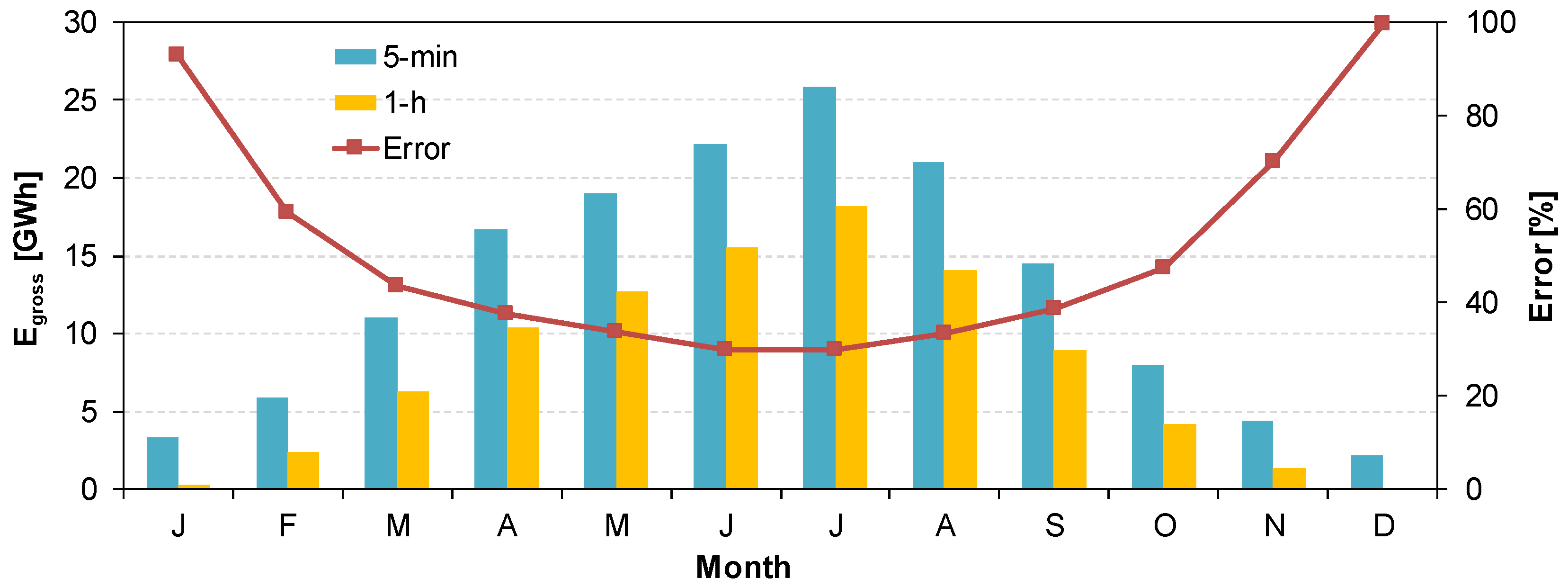
3.3. Annual Power and Freshwater Comparison
4. Conclusions
Author Contributions
Funding
Institutional Review Board Statement
Informed Consent Statement
Data Availability Statement
Acknowledgments
Conflicts of Interest
Nomenclature
| Direct normal irradiance, W/m2 | |
| Gross electric energy, MWh | |
| Thermal energy stored in the TES system, MWh | |
| εE | Relative error in the electric energy produced |
| εqd | Relative error in the freshwater produced |
| Gross electric power, MW | |
| Useful thermal power obtained from the solar field, MW | |
| Excess of thermal power in the solar field, MW | |
| Thermal power sent from the TES system to the power block, MW | |
| Mass flow rate of steam in the first cell of the MED unit, kg/s | |
| Freshwater volume produced in the MED unit, m3 | |
| Heat transfer fluid temperature in SCA , °C | |
| Temperature margin from the design loop outlet temperature (390 °C) | |
| Simulation time step, s | |
| Calculation time, s | |
| Abbreviations | |
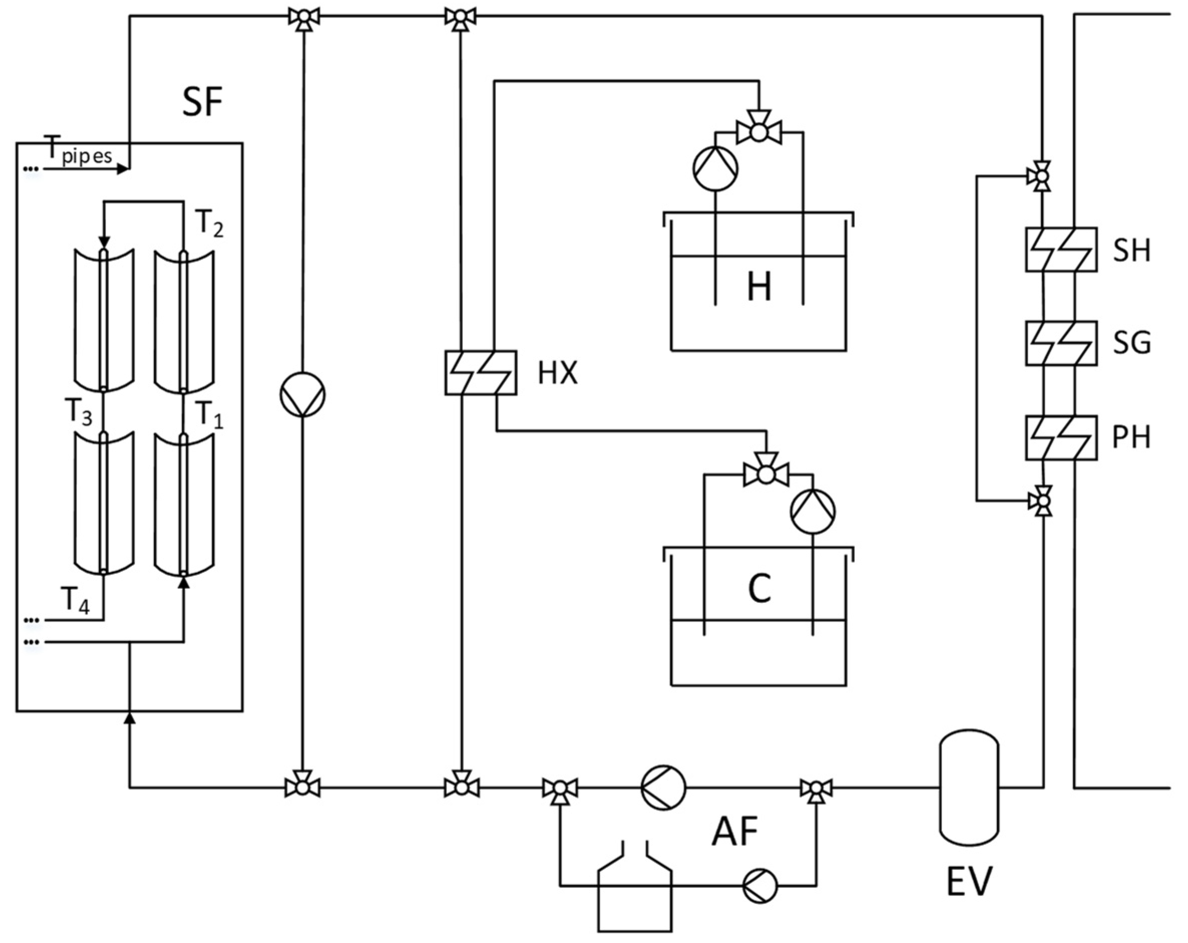
| AF | Anti-freeze |
| C | Cold tank |
| CSP+D | Concentrating solar power and desalination |
| CP | Condensate pump |
| DNI | Direct normal irradiance |
| EV | Expansion vessel |
| FWH | Feedwater heater |
| G | Electric generator |
| GOR | Gain output ratio |
| H | Hot tank |
| HCE | Heat collection element |
| HP | High-pressure turbine |
| HTF | Heat transfer fluid |
| HX | Heat exchanger |
| LP | Low-pressure turbine |
| MED | Multi-effect distillation |
| MP | Main pump |
| LT-MED | Low-temperature multi-effect distillation |
| PH | Preheater |
| PT-CSP | Parabolic trough concentrating solar power |
| RO | Reverse osmosis |
| RH | Reheater |
| SAM | Solar advisor model |
| SCA | Solar collector assembly |
| SCE | Solar collector element |
| SEGS | Solar energy generating system |
| SF | Solar field |
| SG | Steam generator |
| SH | Superheater |
| TES | Thermal energy storage |
| TMY | Typical meteorological year |
References
- IEA World Electricity Final Consumption by Sector, 1974–2019—Charts—Data & Statistics—IEA. Available online: https://www.iea.org/data-and-statistics/charts/world-electricity-final-consumption-by-sector-1974-2019 (accessed on 24 January 2022).
- Palenzuela, P.; Zaragoza, G.; Alarcón-Padilla, D.C.; Guillén, E.; Ibarra, M.; Blanco, J. Assessment of different configurations for combined parabolic-trough (PT) solar power and desalination plants in arid regions. Energy 2011, 36, 4950–4958. [Google Scholar] [CrossRef]
- Palenzuela, P.; Zaragoza, G.; Alarcón, D.; Blanco, J. Simulation and evaluation of the coupling of desalination units to parabolic-trough solar power plants in the Mediterranean region. Desalination 2011, 281, 379–387. [Google Scholar] [CrossRef]
- Sharaf, M.A.; Nafey, A.S.; García-Rodríguez, L. Exergy and thermo-economic analyses of a combined solar organic cycle with multi effect distillation (MED) desalination process. Desalination 2011, 272, 135–147. [Google Scholar] [CrossRef]
- Uche, J.; Valero, A.; Serra, L.; Torres, C. Bblocks software for thermoeconomic analysis of dual-purpose power and desalination plants. Int. J. Thermodyn. 2012, 15, 215–220. [Google Scholar]
- Darwish, M.A.; Darwish, A. Solar cogeneration power-desalting plant with assisted fuel. Desalin. Water Treat. 2014, 52, 9–26. [Google Scholar] [CrossRef]
- Ortega-Delgado, B.; García-Rodríguez, L.; Alarcón-Padilla, D.C. Thermoeconomic comparison of integrating seawater desalination processes in a concentrating solar power plant of 5 MWe. Desalination 2016, 392, 102–117. [Google Scholar] [CrossRef]
- Ortega-Delgado, B.; Palenzuela, P.; Alarcón-Padilla, D.C.; García-Rodríguez, L. Quasi-steady state simulations of thermal vapor compression multi-effect distillation plants coupled to parabolic trough solar thermal power plants. Desalin. Water Treat. 2016, 57, 23085–23096. [Google Scholar] [CrossRef]
- Leiva-Illanes, R.; Escobar, R.; Cardemil, J.M.; Alarcón-Padilla, D.C. Thermoeconomic assessment of a solar polygeneration plant for electricity, water, cooling and heating in high direct normal irradiation conditions. Energy Convers. Manag. 2017, 151, 538–552. [Google Scholar] [CrossRef]
- Calise, F.; Dentice d’Accadia, M.; Vanoli, R.; Vicidomini, M. Transient analysis of solar polygeneration systems including seawater desalination: A comparison between linear Fresnel and evacuated solar collectors. Energy 2019, 172, 647–660. [Google Scholar] [CrossRef]
- Walkenhorst, O.; Luther, J.; Reinhart, C.; Timmer, J. Dynamic annual daylight simulations based on one-hour and one-minute means of irradiance data. Sol. Energy 2002, 72, 385–395. [Google Scholar] [CrossRef] [Green Version]
- Bonilla, J.; Yebra, L.J.; Dormido, S.; Zarza, E. Parabolic-trough solar thermal power plant simulation scheme, multi-objective genetic algorithm calibration and validation. Sol. Energy 2012, 86, 531–540. [Google Scholar] [CrossRef]
- Lippke, F. Simulation of the Part-Load Behavior of a 30 MWe SEGS Plant; Sandia National Lab. (SNL-NM): Albuquerque, NM, USA, 1995.
- Wagner, M.J.; Zhu, G. Generic CSP Performance Model for NREL’s System Advisor Model; National Renewable Energy Lab. (NREL): Golden, CO, USA, 2011.
- Wagner, P.H. Thermodynamic Simulation of Solar Thermal Power Stations with Liquid Salt as Heat Transfer Fluid. Ph.D. Thesis, Technische Universität München, München, Germany, 2012. [Google Scholar]
- Casimiro, S.; Cardoso, J.; Ioakimidis, C.; Farinha Mendes, J.; Mineo, C.; Cipollina, A. MED parallel system powered by concentrating solar power (CSP). Model and case study: Trapani, Sicily. Desalin. Water Treat. 2015, 55, 3253–3266. [Google Scholar] [CrossRef] [Green Version]
- Moser, M.; Trieb, F.; Fichter, T.; Kern, J.; Hess, D. A flexible techno-economic model for the assessment of desalination plants driven by renewable energies. Desalin. Water Treat. 2015, 55, 3091–3105. [Google Scholar] [CrossRef]
- Alikulov, K.; Xuan, T.D.; Higashi, O.; Nakagoshi, N.; Aminov, Z. Analysis of environmental effect of hybrid solar-assisted desalination cycle in Sirdarya Thermal Power Plant, Uzbekistan. Appl. Therm. Eng. 2017, 111, 894–902. [Google Scholar] [CrossRef]
- Mata-Torres, C.; Escobar, R.A.; Cardemil, J.M.; Simsek, Y.; Matute, J.A. Solar polygeneration for electricity production and desalination: Case studies in Venezuela and northern Chile. Renew. Energy 2017, 101, 387–398. [Google Scholar] [CrossRef]
- Hoffmann, J.E.; Dall, E.P. Integrating desalination with concentrating solar thermal power: A Namibian case study. Renew. Energy 2018, 115, 423–432. [Google Scholar] [CrossRef]
- Ortega-Delgado, B.; Palenzuela, P.; Alarcón-Padilla, D.C.; García-Rodríguez, L. Yearly simulations of the electricity and fresh water production in PT-CSP+MED-TVC plants: Case study in Almería (Spain). AIP Conf. Proc. 2018, 2033, 160004. [Google Scholar]
- Askari, I.B.; Ameri, M. Solar Rankine Cycle (SRC) powered by Linear Fresnel solar field and integrated with Multi Effect Desalination (MED) system. Renew. Energy 2018, 117, 52–70. [Google Scholar] [CrossRef]
- Palenzuela, P.; Ortega-Delgado, B.; Alarcón-Padilla, D.-C. Comparative assessment of the annual electricity and water production by concentrating solar power and desalination plants: A case study. Appl. Therm. Eng. 2020, 177, 115485. [Google Scholar] [CrossRef]
- Al-Addous, M.; Jaradat, M.; Bdour, M.; Dalala, Z.; Wellmann, J. Combined concentrated solar power plant with low-temperature multi-effect distillation. Energy Explor. Exploit. 2020, 38, 1831–1853. [Google Scholar] [CrossRef]
- Desai, N.B.; Pranov, H.; Haglind, F. Techno-economic analysis of a foil-based solar collector driven electricity and fresh water generation system. Renew. Energy 2021, 165, 642–656. [Google Scholar] [CrossRef]
- Suraparaju, S.K.; Sampathkumar, A.; Natarajan, S.K. Experimental and economic analysis of energy storage-based single-slope solar still with hollow-finned absorber basin. Heat Transf. 2021, 50, 5516–5537. [Google Scholar] [CrossRef]
- Suraparaju, S.K.; Dhanusuraman, R.; Natarajan, S.K. Performance evaluation of single slope solar still with novel pond fibres. Process Saf. Environ. Prot. 2021, 154, 142–154. [Google Scholar] [CrossRef]
- Blanco-Marigorta, A.M.; Victoria Sanchez-Henríquez, M.; Peña-Quintana, J.A. Exergetic comparison of two different cooling technologies for the power cycle of a thermal power plant. Energy 2011, 36, 1966–1972. [Google Scholar] [CrossRef]
- Montes, M.J.; Abánades, A.; Martínez-Val, J.M.; Valdés, M. Solar multiple optimization for a solar-only thermal power plant, using oil as heat transfer fluid in the parabolic trough collectors. Sol. Energy 2009, 83, 2165–2176. [Google Scholar] [CrossRef] [Green Version]
- Xu, X.; Vignarooban, K.; Xu, B.; Hsu, K.; Kannan, A.M. Prospects and problems of concentrating solar power technologies for power generation in the desert regions. Renew. Sustain. Energy Rev. 2016, 53, 1106–1131. [Google Scholar] [CrossRef]
- Ortega-Delgado, B.; Cornali, M.; Palenzuela, P.; Alarcón-Padilla, D.C. Operational analysis of the coupling between a multi-effect distillation unit with thermal vapor compression and a Rankine cycle power block using variable nozzle thermocompressors. Appl. Energy 2017, 204, 690–701. [Google Scholar] [CrossRef]
- Llorente García, I.; Álvarez, J.L.; Blanco, D. Performance model for parabolic trough solar thermal power plants with thermal storage: Comparison to operating plant data. Sol. Energy 2011, 85, 2443–2460. [Google Scholar] [CrossRef]
- Eck, M.; Barroso, H.; Blanco, M.; Burgaleta, J.I.; Dersch, J.; Feldhoff, J.-F.; Garcia-Barberena, J.; Gonzalez, L.; Hirsch, T.; Ho, C.; et al. guiSmo: Guidelines for CSP performance modeling—Present status of the SolarPACES Task-1 project. In Proceedings of the 17th SolarPACES Conference, Granada, Spain, 20–23 September 2011. [Google Scholar]
- Ortega-Delgado, B.; García-Rodríguez, L.; Alarcón-Padilla, D.C. Opportunities of improvement of the MED seawater desalination process by pretreatments allowing high-temperature operation. Desalin. Water Treat. 2017, 97, 94–108. [Google Scholar] [CrossRef]
- Klein, S. Engineering Equation Solver Software (EES) 2021. Version 11.212. Available online: https://fchartsoftware.com/ees/ (accessed on 31 January 2022).


| Period | Δt | εE | εqd | |||
|---|---|---|---|---|---|---|
| min | min | GWh | % | hm3 | % | |
| 21–23 June | 5 | 43.59 | 2.19 | - | 48.2 | - |
| 10 | 13.17 | 2.13 | 2.4 | 47.0 | 2.4 | |
| 15 | 4.75 | 2.08 | 4.8 | 45.9 | 4.8 | |
| 30 | 1.02 | 1.93 | 11.9 | 42.5 | 11.8 | |
| 60 | 0.12 | 1.52 | 30.3 | 33.9 | 29.7 |
| Month | 5 min | 1 h | ||||
|---|---|---|---|---|---|---|
| εE | εqd | |||||
| GWh | ×103 m3 | GWh | ×103 m3 | % | % | |
| January | 3.35 | 80.5 | 0.24 | 6.4 | 92.8 | 92.1 |
| February | 5.84 | 131.8 | 2.37 | 56.2 | 59.3 | 57.3 |
| March | 11.01 | 249.0 | 6.23 | 140.6 | 43.4 | 43.5 |
| April | 16.67 | 373.0 | 10.41 | 219.9 | 37.6 | 41.1 |
| May | 19.04 | 424.9 | 12.64 | 280.8 | 33.6 | 33.9 |
| June | 22.16 | 495.5 | 15.52 | 343.4 | 30.0 | 30.7 |
| July | 25.85 | 578.0 | 18.12 | 398.9 | 29.9 | 31.0 |
| August | 21.00 | 465.4 | 14.01 | 310.3 | 33.3 | 33.3 |
| September | 14.47 | 321.0 | 8.87 | 197.8 | 38.7 | 38.4 |
| October | 7.97 | 179.1 | 4.20 | 98.6 | 47.3 | 44.9 |
| November | 4.40 | 102.5 | 1.32 | 34.0 | 70.1 | 66.8 |
| December | 2.19 | 52.9 | ≈0 | 0.2 | 99.7 | 99.7 |
| Year | 153.95 | 3453.7 | 93.94 | 2087.1 | 39.0 | 39.6 |
Publisher’s Note: MDPI stays neutral with regard to jurisdictional claims in published maps and institutional affiliations. |
© 2022 by the authors. Licensee MDPI, Basel, Switzerland. This article is an open access article distributed under the terms and conditions of the Creative Commons Attribution (CC BY) license (https://creativecommons.org/licenses/by/4.0/).
Share and Cite
Ortega-Delgado, B.; Palenzuela, P.; Alarcón-Padilla, D.-C. Analysis of the Time Step Influence in the Yearly Simulation of Integrated Seawater Multi-Effect Distillation and Parabolic trough Concentrating Solar Thermal Power Plants. Processes 2022, 10, 573. https://doi.org/10.3390/pr10030573
Ortega-Delgado B, Palenzuela P, Alarcón-Padilla D-C. Analysis of the Time Step Influence in the Yearly Simulation of Integrated Seawater Multi-Effect Distillation and Parabolic trough Concentrating Solar Thermal Power Plants. Processes. 2022; 10(3):573. https://doi.org/10.3390/pr10030573
Chicago/Turabian StyleOrtega-Delgado, Bartolomé, Patricia Palenzuela, and Diego-César Alarcón-Padilla. 2022. "Analysis of the Time Step Influence in the Yearly Simulation of Integrated Seawater Multi-Effect Distillation and Parabolic trough Concentrating Solar Thermal Power Plants" Processes 10, no. 3: 573. https://doi.org/10.3390/pr10030573