The Engine Combustion Phasing Prediction Based on the Support Vector Regression Method

Abstract

While traditional one-dimensional and three-dimensional numerical simulation techniques require a lot of tests and time, emerging Machine Learning (ML) methods can use fewer data to obtain more information to assist in engine development. Combustion phasing is an important parameter of the spark-ignition (SI) engine, which determines the emission and power performance of the engine. In the engine calibration process, it is necessary to determine the maximum brake torque timing (MBT) for different operating conditions to obtain the best engine dynamics performance. Additionally, the determination of the combustion phasing enables the Wiebe function to predict the combustion process. Existing studies have unacceptable errors in the prediction of combustion phasing parameters. This study aimed to find a solution to reduce prediction errors, which will help to improve the calibration accuracy of the engine. In this paper, we used Support Vector Regression (SVR) to reconstruct the mapping relationship between engine inputs and responses, with the hyperparametric optimization method Gray Wolf Optimization (GWO) algorithm. We chose the engine speed, load, and spark timing as engine inputs. Combustion phasing parameters were selected as engine responses. After machine learning training, we found that the prediction accuracy of the SVR model was high, and the R² of CA10−ST, CA50, CA90, and DOC were all close to 1. The RMSE of these indicators were close to 0. Consequently, SVR can be applied to the prediction of combustion phasing in SI gasoline engines and can provide some reference for combustion phasing control.

1. Introduction

As carbon peak emissions and carbon-neutral strategies continue to advance, higher demands are being placed on engine performance [1,2]. The internal combustion engines will continue to be the major power sources, especially for heavy-duty trucks and off-road applications [3,4]. The new requirements of next generation engines are more efficient and cleaner combustion [5,6,7]. The use of updated tools to assist engine design, which can shorten the period of engine design and reduce development costs, is a new trend [8,9]. In the process of engine research and development, numerical simulation is often used to assist the design [10,11], thus improving the efficiency of development and reducing the number of tests. Three-dimensional (3D) simulation technology can simulate the flow and combustion processes in the cylinder well [12,13]. However, it requires complex chemical mechanisms and high computational power, which makes 3D simulation computationally expensive [14,15]. Zero-dimensional (0D) and one-dimensional (1D) simulation techniques, focusing on the overall performance of the powertrain [16], can be used to analyze in-cylinder heat transfer. Semi-empirical models, such as Wiebe functions [17], are used for combustion calculations. Compared with 3D simulation technology, 1D simulation requires less calculation time but more test data for calibrations [18]. More recently, with the development of machine learning (ML) and computer performance, data-driven surrogate models have become an approach to engine development [19,20,21]. ML models do not require complex physical models, they are reconstructions of the engine input and output relationships and reduce the number of tests [22]. The prediction of output parameters is used to help the engine development process. Such as engine power performance [23,24,25], emission performance [19,26], exhaust gas temperature [27,28].

Combustion phasing parameters are vital to engine combustion control [29,30,31]. The combustion phasing parameters reflect the in-cylinder combustion and determine the dynamic performance and emissions of the engine [32,33]. The combustion phasing parameters help to search for maximum brake torque (MBT) timing, under which the engine will have the best dynamic performance and the lowest fuel consumption rate. Therefore, during engine calibration, the combustion phasing parameters should be controlled. For example, the crank angle where 50% of fuel has burnt (CA50) should be limited in the range of 5 to 11 CAD ATDC for most ignition engines [30]. Determining the optimal combustion phasing is the primary work to be done during engine calibration, which obtains a balance between engine efficiency and emissions. Traditionally, the engine calibration work is carried out by dynamometer tests, which are time consuming and expensive [34]. Worse, the engine dynamometer tests may output different performances at different times, such as the different weather and different seasons [35]. Additionally, the unavoidable noise from the experimental tests also contributes to the uncertainties [36]. Furthermore, combustion phasing is required for a robust Wiebe function. The Wiebe function can only predict the combustion in the cylinder if accurate combustion phase parameters are provided [37]. Generally, the prediction of combustion phasing is a key technology.

Therefore, a fast and efficient tool to assist engine mapping is needed to reduce costs and effort. The machine learning approach has been approved to be such a tool because it can eliminate the noise and effectively establish the relationship between engine operational parameters and engine responses [38,39]. In recent years, many researchers have combined machine learning methods to predict the combustion process [40,41] and to control the combustion phasing parameters of engines [42,43]. Edward et al. [44] applied a clustering method based on fuzzy logic predicates to the combustion stage identification of internal combustion engines. Huanyu et al. [45] adopted an extreme learning machine (ELM) to learn and estimate the in-cylinder pressure sequence in the combustion process and combustion stage. They controlled the in-cylinder combustion in real-time by controlling the combustion phasing. Wang et al. [46] established the oxidizer temperature, pressure, and mixture fraction for a dual-fuel engine by using high-dimensional input-output relationship (HDMR) and Convolutional Neural Networks (CNN) methods. The relationship between strain rate and ignition delay showed that machine learning methods could capture the ignition behavior of dual-fuel engines. Liu et al. used random forest (RF) [47] and K-nearest Neighbors (KNN) algorithms [48] to predict CA50 and the location of peak cylinder pressure of a natural gas engine. However, the error of the prediction results is slightly larger in the existing studies, which may affect the calibration accuracy. In terms of combustion phase parameter prediction, according to the literature, the prediction accuracy of the RF [47] and KNN [48] methods are not high enough, with the RMSE around 3 CAD. The ANN method can reduce the RMSE to 1.4 CAD [24], but such predictions are still difficult to use for accurate engine calibration and robust Wiebe function modification. Generally, these machine learning methods have limited accuracy in predicting combustion phasing.

Support Vector Regression (SVR) is a suitable machine learning method for nonlinear and complex regression problems [49,50], based on Support Vector Machine (SVM). Moreover, it has some applications in engine responses prediction [22,51]. Najafi et al. [52] used SVR model to establish the relationship between engine fuel composition and emissions. As shown in

Table 1. The application of SVR model for different engine parameters prediction.

Study	Engine Type	Input	Output	Performance (R2)
[53]	Diesel engine	Rail pressure, Injection timing, Charge pressure, Charge temperature, Max pressure	Max pressure	0.99
[54]	Diesel engine	Speed, brake mean effective pressure (BMEP)	Soot emissions	0.97
[55]	Hydrogen enriched engine	Excess air ratio, speed, injection timing, Fuel, hydrogen volume percentage	Cyclic variation of speed	0.99
[56]	Diesel engine	Engine speed, amount of injected fuel, rail pressure, BMEP	BMEP	0.99
[57]	Hydrogen enriched engine	Excess air ratio, hydrogen volume percentage, injection timing	CO emissions	0.99
[58]	Diesel engine	Injection pressure, injection timing	Max pressure	0.99

, SVR performs well in predicting many engine parameters, however, at present. However, SVR model is seldom used to predict the combustion phasing of spark ignition (SI) gasoline engines. Consequently, the goal of this study is to find a solution to reduce the prediction error, which can help improve the calibration accuracy of engines.

In this paper, the application of SVR-GWO algorithm in engine combustion phasing parameters prediction was discussed, which contributed to the determination of MBT and the modification of the Wiebe function. A calibrated 1D model of the SI gasoline engine was developed and simulation experiments were performed. Then, the SVR algorithm was used for fitting and the Gray Wolf Optimization (GWO) algorithm [59] was used to optimize the hyperparameter set. The engine speed, load, and spark timing were used to model the engine combustion phasing parameters. The prediction results were compared with the 1D simulation results. Finally, the prediction curves of engine performance and engine input parameters were generated based on the SVR model.

2. Data Collection and ML Modeling

2.1. SI Engine Setup

A single-cylinder 0.5 L SI gasoline engine with natural suction and port fuel injection was selected to study in this research. GT-Power software was used for the numerical simulation software [60]. Based on the actual engine geometry parameters, the structural dimensions of the 1D simulation model are determined as inputs [61], including the cylinder diameter, stroke, and compression ratio of the engine, as shown in Figure 1. The important parameters are shown in

Table 2. Engine specifications.

Engine Type	Single-Cylinder 4-Stroke SI Gasoline Engine
Stroke × Bore	86.07 mm × 86 mm
Intake valve open	9 CAD BTDC
Intake valve close	84 CAD ABDC
Exhaust valve open	55 CAD BBDC
Exhaust valve close	38 CAD ATDC
Compression ratio	9.5
Connecting rod length	175 mm

. The calibration of this simulation model can be seen in the relevant study [62]. GT-Power has several numerical simulation models for simulating the complex in-cylinder combustion processes in internal combustion engines, among which the “EngCylCombSITurb” [63] predictive turbulent combustion model is used in the numerical simulations. In the simulation model, “flame kernel growth multiplier” (FKMG) and “turbulent flame speed multiplier” (TFSM) are two key parameters. By adjusting these parameters, the combustion phasing in the engine cylinder can be calculated accurately.

In this paper, CA10 is the crank angle (CA) where 10% fuel burnt, and CA10−ST (the duration between spark timing to CA10) represents ignition delay. CA50 is the CA where 50% of fuel burnt, representing the middle point of combustion. CA90 is the CA where 90% of fuel burnt, representing the moment when the combustion finishes. DOC is the combustion duration defined by the duration between CA10 to CA90. These combustion phasing parameters can be calculated by a 1D model calculation of GT-Power.

To obtain the input data set for the ML method, three engine input parameters were selected: engine speed, load (controlled by intake pressure), and spark timing, as shown in

Table 3. Simulation setup.

Title	Range	Step
Engine speed	1000~4000 RPM	200 RPM
Intake pressure	0.5~1 bar	0.1 bar
Spark timing	−40~0 CAD ATDC	2 CAD

. The engine speed was set from 1000 to 4000 RPM with 200 RPM intervals. The intake pressure was set from 0.5 to 1 bar with 0.1 bar intervals. The spark timing was set from −40 to 0 CAD ATDC with 2 CAD intervals, as shown in Table 3.

As shown in Figure 2, the 1D simulation model in GT-Power was calibrated, and then the data was calculated from the 1D model, without noise [58]. We used the training dataset to build the ML surrogate model. Since this paper focused on the applicability of machine learning methods, the data must be free from noise caused by experiments, so that the sources of prediction errors can be analyzed. In this way, the ability of machine learning methods to predict the combustion phasing parameters can be judged.

2.2. SVR Method

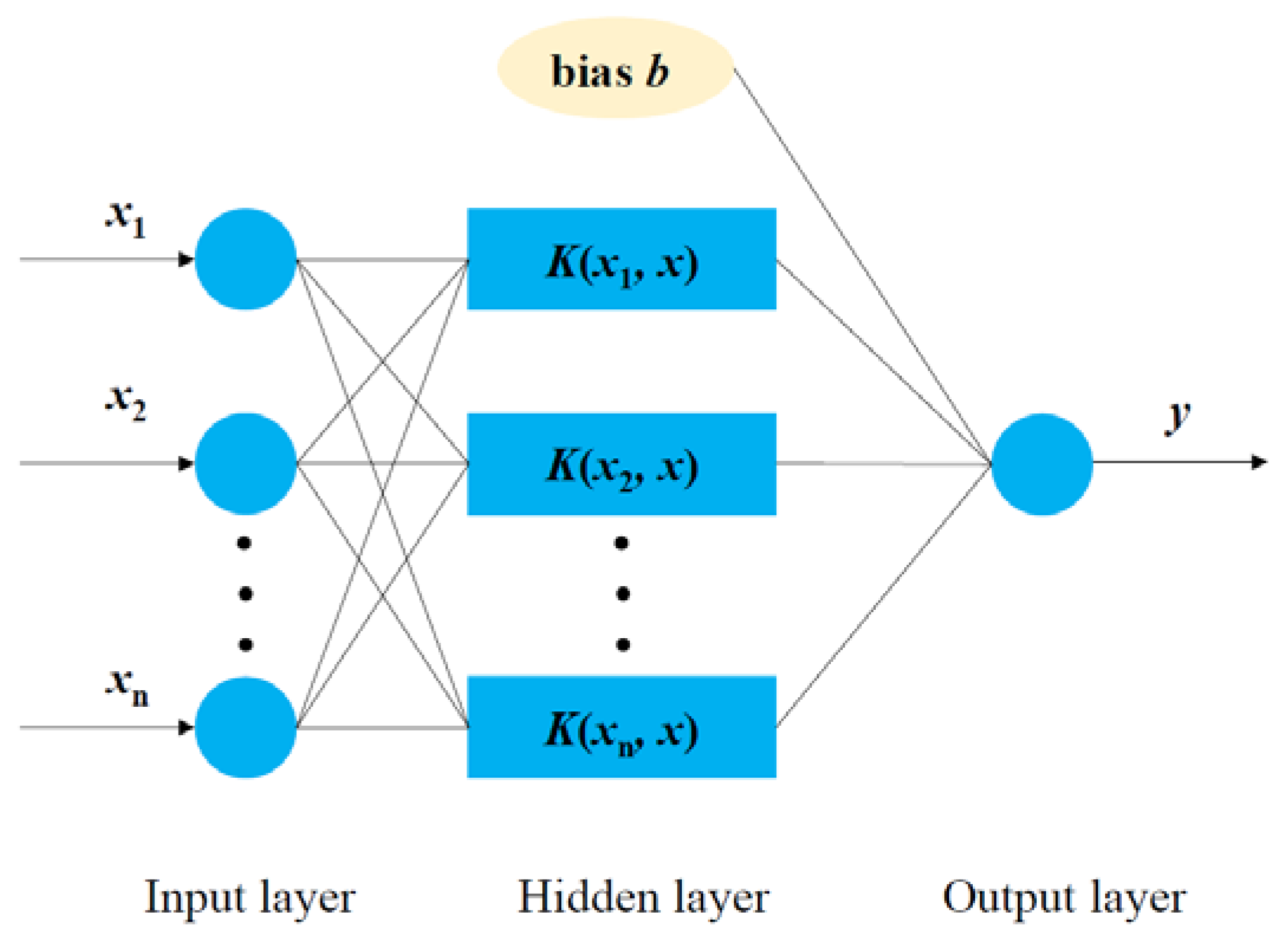
SVR is a model derived from SVM and its structure is similar to ANN [64], as shown in Figure 3. The structure of SVR has an input layer, hidden layer, and output layer. By learning the training dataset of the input layer, the parameters of the hidden layer can be obtained automatically.

By using kernel functions in the SVR model, feature vectors of sample data can be mapped from low dimension to high dimension. The hyperplane which brings all the data in a set to the closest distance to the plane can be found, as shown in Figure 4. $\epsilon$ represents the maximum deviation.

The regression function of the SVM is shown below:

$$\begin{array}{c}f\left(x\right)=\omega ·x+b\end{array}$$

(1)

where $\omega$ and $b$ are the hyperplane coefficients; $x$ is the input feature vector; and f(x) represents the predicted value of the input feature vector.

To find the most value regression function, the soft marginal loss function (SMLF) is established [56]:

$$\begin{array}{c}min\frac{1}{2}{\omega }^T\omega +C\frac{1}{N}{\displaystyle {\displaystyle \sum }_{i=1}^N}{L\left(f\right(x}_i{),y}_i)\end{array}$$

(2)

$$\begin{array}{c}L\left(y\right)=\{\begin{array}{c}0,\left|f\left(x_i\right)-y_i\right|\le \epsilon \\ \left|f\left(x_i\right)-y_i\right|-\epsilon ,\left|f\left(x_i\right)-y_i\right|\ge \epsilon \end{array}\end{array}$$

(3)

where $C$ represents the penalty factor; $y$ represents the true value; and L represents the loss function.

When slack variables $\xi$ and ${\xi }_i^{\star }$ are introduced to the problem, Equation (4) can be expressed as [65]:

$$min\frac{1}{2}{\omega }^T\omega +C{\displaystyle \sum }_{i=1}^n\left({\xi }_i{+\xi }_i^{\star }\right)$$

$$\begin{array}{c}s.t.\{\begin{array}{c}{y}_i-\omega ·x_i-b\le {\epsilon +\xi }_i\\ y_i-\omega ·x_i-b\le {\epsilon +\xi }_i^{\star }\\ {\xi }_i{,\xi }_i^{\star }\ge 0\end{array}\end{array}$$

(4)

By establishing the Lagrangian function and the Karush Kuhu Tucker (KKT) condition [66], the final regression function can be expressed as:

$$\begin{array}{c}f\left(x\right)=\omega ·x+b={\displaystyle {\displaystyle \sum }_{i=1}^l}\left(a_i-a_i^{*}\right)K\left(x_i·x\right)+b\end{array}$$

(5)

where $l$ is the number of SVR machines; ${\alpha }_i$ represents the optimal solution; and $K$ is the kernel function, when satisfying the Mercer condition [40], K(x_i, x) = $\Phi$(x_i)·$\Phi$(x_j).

Among the kernel functions, RBF can reflect the nonlinear response of the engine well [40]. Therefore, RBF was chosen in this paper, and by adjusting the kernel function coefficients $\gamma$, RBF would have high flexibility. The function can be expressed as [50]:

$$\begin{array}{c}K\left(x_i{,x}_j\right)=exp\left({-\gamma |x}_i-x_j{|}^2\right),\gamma >0\end{array}$$

(6)

Most importantly, the penalty factor C, the kernel function coefficient $\gamma$, and the maximum deviation $\epsilon$ will all affect the result of SVR [67]. These parameters can be set in the LibSVM [68], which is an efficient SVM regression learning toolbox written by Professor Lin Chih-Jen.

2.3. Gray Wolf Optimization Method

The Gray Wolf Optimization (GWO) algorithm is a novel intelligent operational optimization algorithm proposed by Mirjalili et al. [59] for simulating the hunting behavior of wolves. Generally, the three gray wolves with the highest fitness value were regarded as $\alpha$,$\beta$, and $\gamma$ wolf. Their values determine the optimization process.

The three main definitions of the GWO algorithm are as follows.

Before predation, the position of the prey needs to be determined first; that is, the distance between the prey and gray wolf needs to be solved [59]:

$$\begin{array}{c}D=\left|C{X}_p\left(t\right)-X\left(t\right)\right|\end{array}$$

(7)

where D is the distance between a gray wolf and its prey; $X_p$ is the position vector of prey; $X$ is the position vector of a gray wolf; and C is the coefficient vector, ${C=2r}_1$, $r_1\in (0,1)$.

Then, the position vector of the next generation of gray wolves $X\left(t+1\right)$ is obtained as [59]:

$$\begin{array}{c}X\left(t+1\right){=X}_p\left(t\right)-\mu D\end{array}$$

(8)

$$\begin{array}{c}\mu =2a{r}_2-a\end{array}$$

(9)

where $\mu$ is the convergence vector; and $r_2$ is a random vector of $a$. The component of $a$ has an initial value of 2 and decreases to 0 as the number of iterations increases.

The α wolf is closest to its prey. The distance between other gray wolves and $\alpha$,$\beta$ wolves, and $\gamma$ wolves is as follows [59]:

$$\begin{array}{c}{D}_k=\left|C_i{X}_k\left(t\right)-X\left(t\right)\right|\end{array}$$

(10)

$$\begin{array}{c}{X}_i{=X}_k-{\mu }_i{D}_k\end{array}$$

(11)

$$\begin{array}{c}{X}_p\left(t+1\right)=\frac{X_1{+X}_2{+X}_3}{3}\end{array}$$

(12)

where $k=\alpha ,\beta ,\gamma$; and $i=1,2,3$.

2.4. Data Processing

Normalization can reduce the span of data and improve the accuracy of prediction in ML methods. Therefore, in this research, the normalization method of [−1, 1] was chosen, which can be shown as:

$$\begin{array}{c}y=2\times \left(\frac{x-x_{min}}{x_{max}-x_{min}}\right)-1\end{array}$$

(13)

where x and y are the basic data and normalized data, respectively. After obtaining the ML prediction results, it is necessary to perform the inverse normalization operation.

To evaluate the performance of the SVR method, the dataset generated by the 1D simulation was divided into the training data (80%) and validation data (20%) sets, as shown in Figure 5. Studies by [69,70] indicated that this percentage separation was recommended for the engine model in this research.

To further evaluate the success of the training model, steady-state data sets were utilized, as shown in Figure 5. At 1 bar intake pressure, combustion phasing predictions under different spark timings with certain speeds (i.e., 1000, 2600, and 4000 RPM) were analyzed. Additionally, at −20 CAD ATDC spark timing, combustion phasing predictions under different speeds with certain loads (i.e., 0.6, 0.8, and 1.0 bar) were analyzed. Furthermore, at 2600 RPM, combustion phasing predictions under different loads with certain spark timings (i.e., −40, −20, and 0 CAD ATDC) were analyzed.

The statistical determination coefficient (R²) and root mean square error (RMSE) can be used to evaluate the prediction performance. R² and RMSE are defined as follows:

$${\mathrm{R}}^2=\frac{{\sum }_{i=1}^n{(\widehat{y_i}-\overline{y})}^2}{{\sum }_{i=1}^n{(y_i-\overline{y})}^2}$$

(14)

$$\begin{array}{c}\mathrm{RMSE}=\sqrt{\frac{1}{n}{\displaystyle {\displaystyle \sum }_{i=1}^n}{\left|y_i-\widehat{y_i}\right|}^2}\end{array}$$

(15)

where $\widehat{y_i}$ is the data predicted by SVR model; $\overline{y}$ is the average value of the experimental data; $y_i$ is the measured data; and n is the amount of data. When R² and RMSE are close to 1 and 0, respectively, it means that the predicted value matches well with the measured value and the prediction is accurate.

The process of building the SVR-GWO model is shown in Figure 6. First, the data are preprocessed, including loading and normalization, and then the optimal set of hyperparameters is obtained by the GWO algorithm. Finally, the predictive capability of the SVR model obtained by training is evaluated and de-normalization will be carried out.

3. Results and Discussion

3.1. Combustion Phasing Prediction

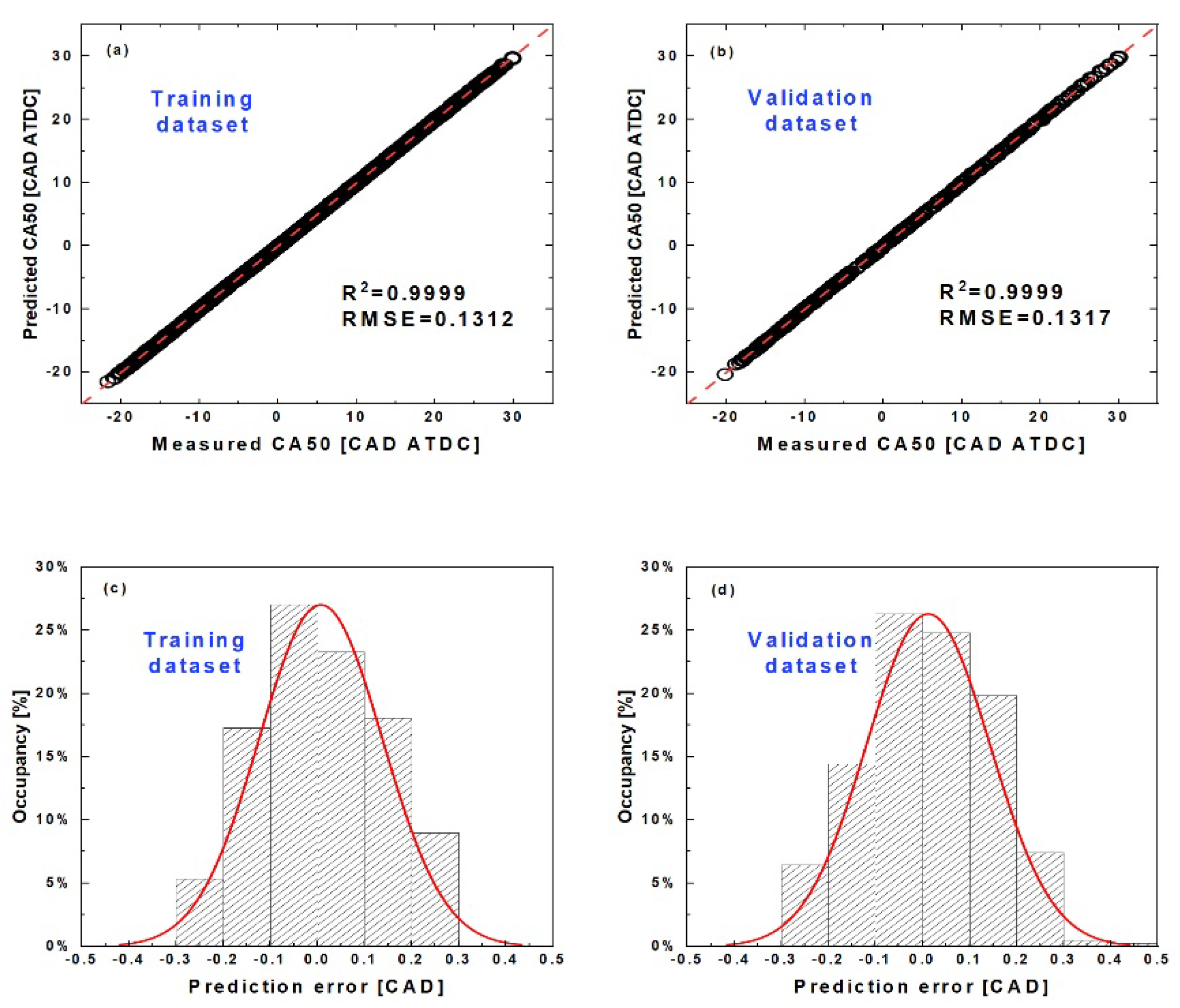
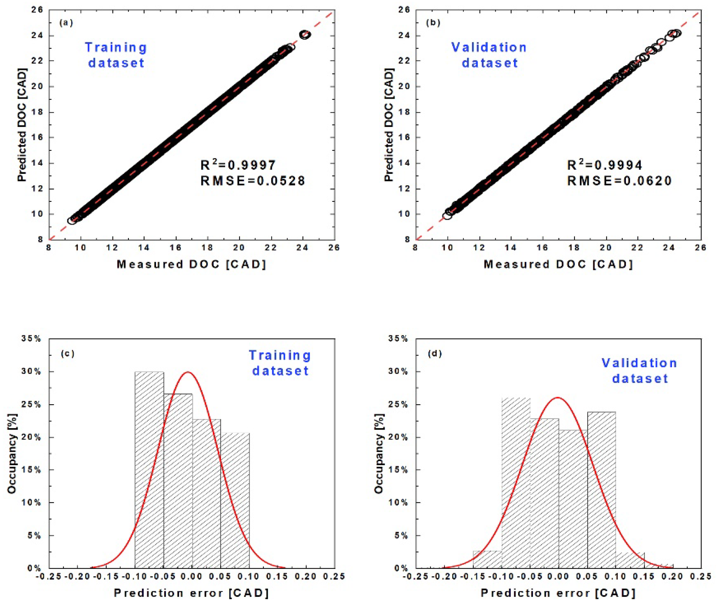
Figure 7, Figure 8, Figure 9 and Figure 10 show the comparison of the measured data with SVR prediction results and the distribution of prediction errors. The choice of hyperparameters is shown at the top of each figure. Study [55] shows that, as the value of $\epsilon$ decreases, the calculation amount of the model will increase, but when the value of $\epsilon$ increases, the prediction accuracy of the model will decrease, so the selection of $\epsilon$ is 0.01. The selection of C and γ was obtained by GWO algorithm.

$$\mathrm{Hyperparameter}\mathrm{set}:C=289.58;\gamma =2.88;\epsilon =0.01$$

$$\mathrm{Hyperparameter}\mathrm{set}:C=82.88;\gamma =0.23;\epsilon =0.01$$

$$\mathrm{Hyperparameter}\mathrm{set}:C=178.82;\gamma =0.39;\epsilon =0.01$$

$$\mathrm{Hyperparameter}\mathrm{set}:C=235.18;\gamma =2.51;\epsilon =0.01$$

For the training dataset, the R² of CA10−ST, CA50, CA90, and DOC were 0.9996, 0.9999, 0.9999, and 0.9997, respectively. The RMSE of these indicators were 0.0332 CAD, 0.1312 CAD, 0.1788 CAD, and 0.0528 CAD. As for the validation dataset, the R² of CA10−ST, CA50, CA90, and DOC were 0.9994, 0.9999, 0.9999, and 0.9994, respectively. The RMSE of these indicators were 0.0437 CAD, 0.1317 CAD, 0.1867 CAD, and 0.0620 CAD. SVR predicted each indicator accurately, especially CA50 and CA90, with R² very close to 1. This is mainly due to the low noise of the simulated experimental data, so the fluctuation of the results is also small. The prediction performance of SVR model was better than RF, KNN, and ANN [24,47,48]. The SVR method could learn the principle of data variation well. In terms of error distribution, the errors of CA10−ST and DOC are small with the maximum errors less than 0.2 CAD, while the maximum errors of both CA50 and CA90 are larger than 0.3 CAD. This was because CA50 and CA90 increased significantly with the delay of spark timing, resulting in a larger span of their data and a larger prediction error. For each parameter, the prediction results of the training dataset exceeded those of the validation dataset, but the differences were small, indicating that the model generalization ability of SVR was strong.

3.2. Steady-State Prediction

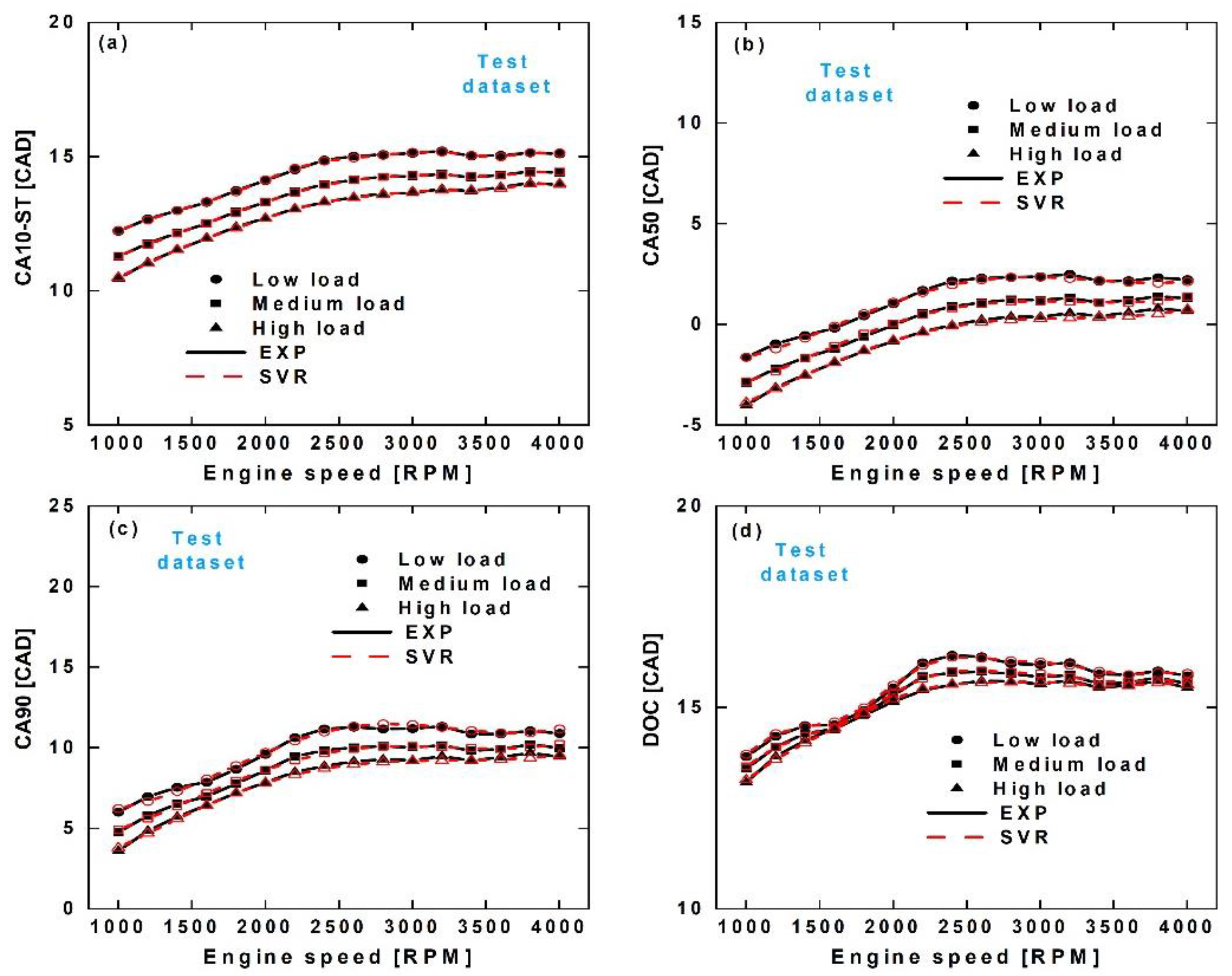
In the previous section, the prediction accuracy of SVR model for each parameter was evaluated from the perspective of statistical results. To investigate whether the SVR model learned the complex combustion process, this section presents a comparison of simulated experimental data and model predictions under different operating conditions. Based on the test dataset divided in Section 2.4, the prediction performance of the SVR model with different operating conditions was discussed.

Figure 11 shows the comparison between calibrated simulation experimental data and SVR model for the effect of spark timing on the combustion phasing. CA10−ST first decreased, and then increased with the spark timing delay, as shown in Figure 11a. CA50 increased with the delay of spark timing, as shown in Figure 11b. The optimum CA50 for a normal internal combustion engine is from 5 to 11 CAD ATDC [30]. Since the SVR model has good predictive performance, it can be used to help select the best spark timing for different operating conditions. The trends of CA90 and DOC were similar. As shown in Figure 11d, when the spark timing increased above −10 CAD ATDC, the DOC in the medium speed condition exceeds that in the high-speed condition. This was because, under high-speed conditions, the lag time of combustion increased with the delay of sparking timing. Generally, SVR model can successfully capture these changes.

Figure 12 shows the comparison between calibrated simulation experimental data and SVR model for the effect of engine speed on the combustion phasing. When the speed increased from 1000 to 2600 RPM, the combustion phasing parameters increased; when the speed increased above 2600 RPM, the combustion phasing did not change significantly. It can be seen that the effect of engine speed was limited because the flame propagation speed increased less when the engine speed increased. Additionally, the prediction accuracy of CA50 and CA90 was lower than that of CA10−ST and DOC. Under certain conditions, the predicted values deviated from the experimental values. This indicates that SVR has some limitations in learning the speed influence law, but in general, it can predict accurately.

Figure 13 shows the comparison between calibrated simulation experimental data and SVR model for the effect of intake pressure on the combustion phasing. It can be seen that the combustion phase parameter decreased as the inlet pressure increased. This was because the airflow velocity increased with the increasing intake pressure, which improved the speed of flame front surface propagation. Therefore, the values of CA10−ST and DOC decreased, while the timing of CA50 and CA90 appeared in advance.

3.3. Engine Map Prediction

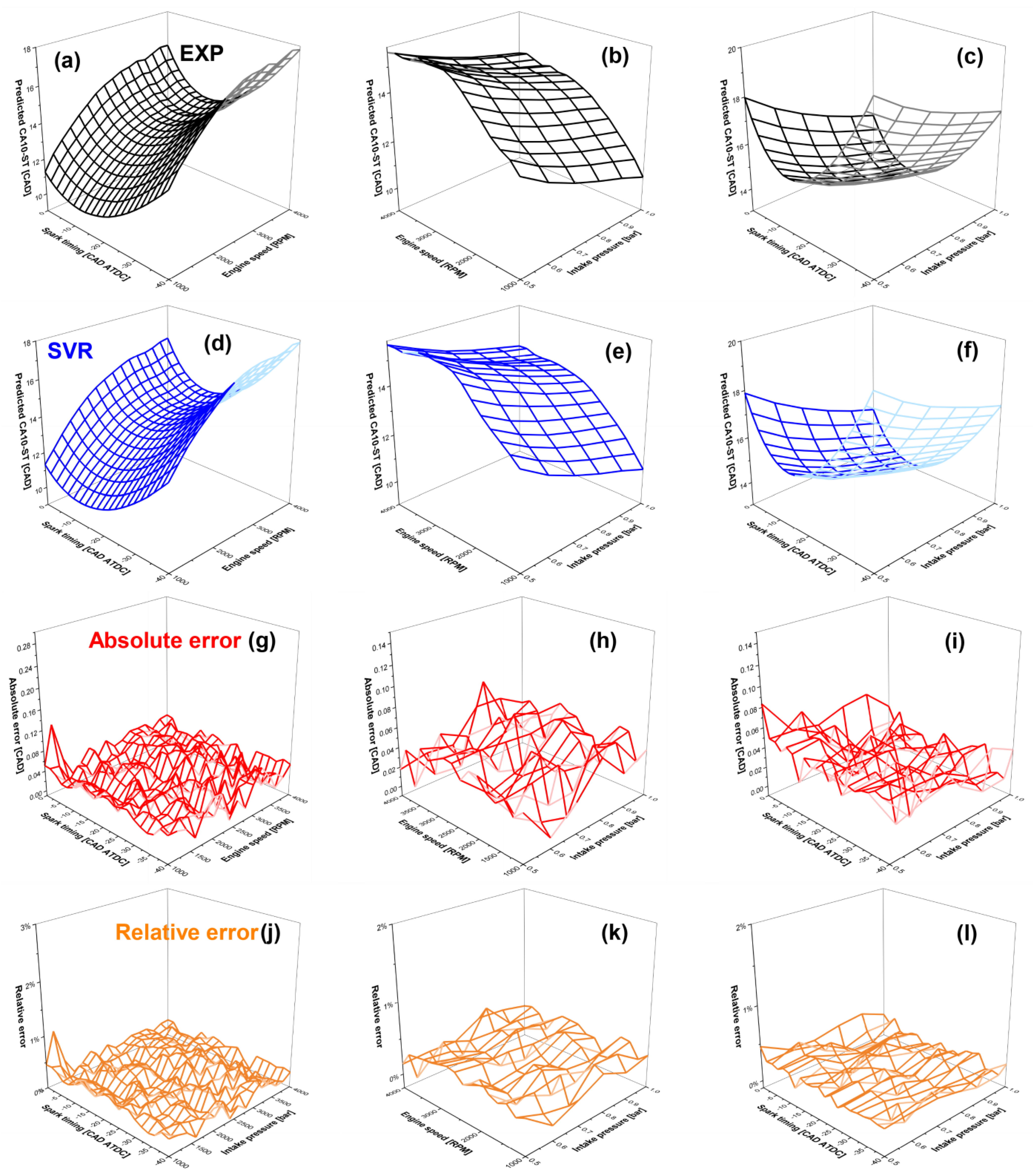
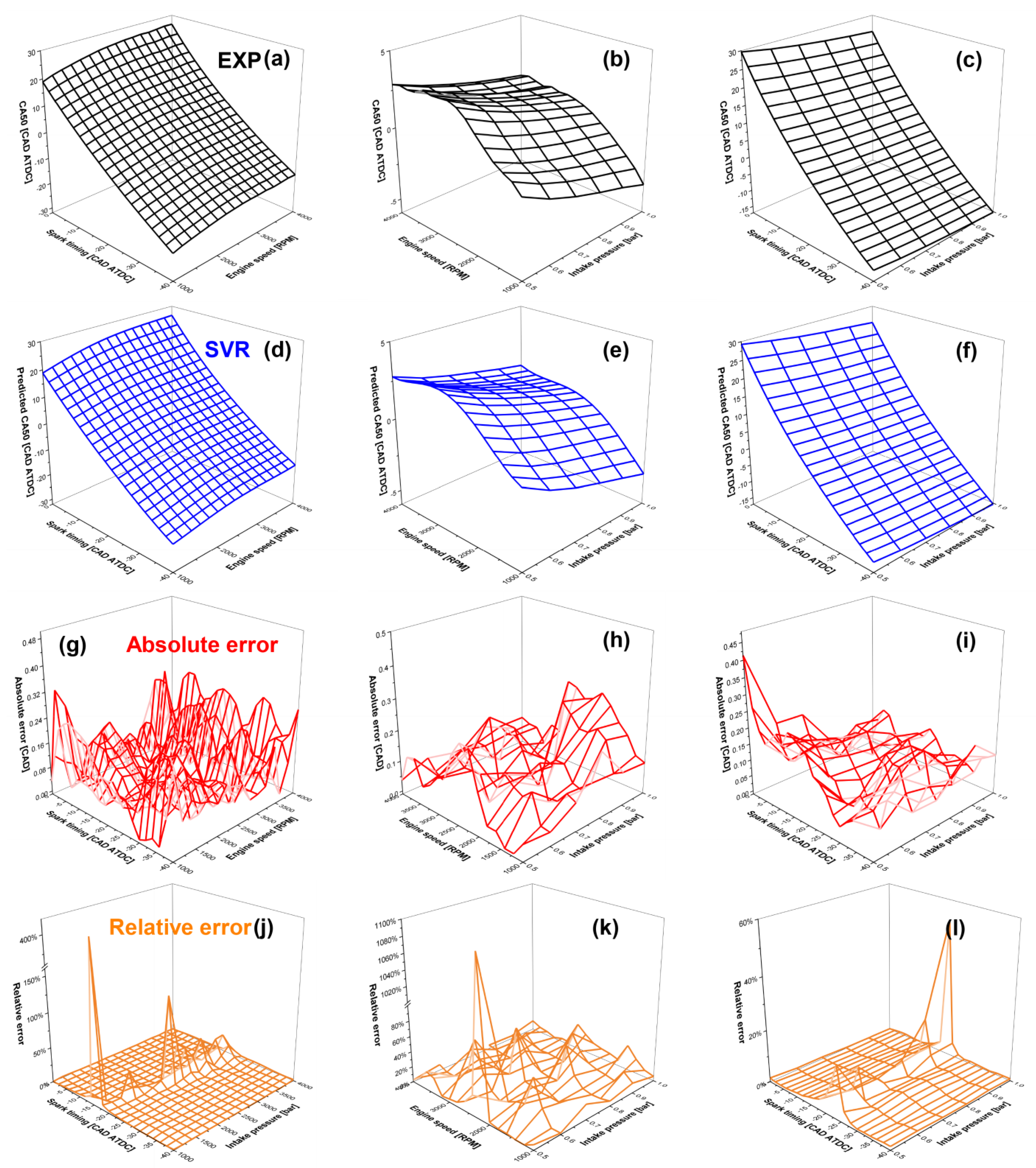
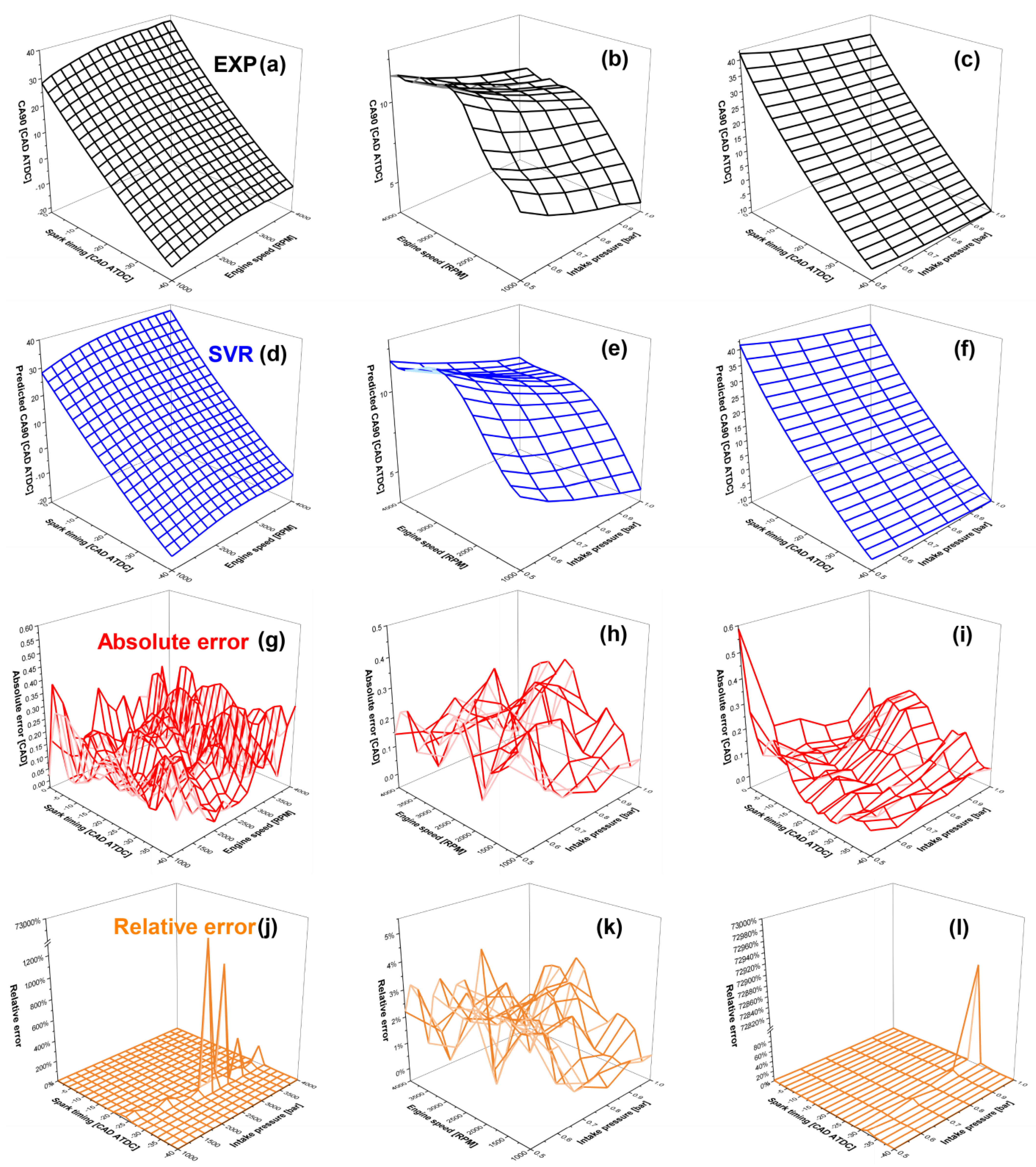
In Section 3.3, SVR model can learn the combustion phasing variation under different operating conditions. In engine calibration, combustion phasing parameters are often used to assist in the determination of MBT. When the spark timing is MBT, the engine is in optimal condition, with maximum torque and minimum fuel consumption. When the spark timing advances, it will make the engine cylinder do more work in the compression stroke, resulting in a waste of energy. On the contrary, when the spark timing is delayed, the piston will locate in the expansion stroke and the in-cylinder pressure of the engine will drop, which is not conducive to the full development of combustion and increases fuel consumption. To reflect the relationship between combustion phasing parameters and operation parameters, The engine map of combustion phasing was predicted by using the SVR model, as shown in Figure 14, Figure 15, Figure 16 and Figure 17.

As shown in Figure 14, CA10−ST decreased with the increasing intake pressure and slightly increased with increasing engine speed. Under different operation conditions, there was a spark timing to minimize CA10−ST. The smaller CA10−ST means a shorter flame development period, more stable engine operation, and less pressure fluctuation between cycles [70].

As shown in Figure 15 and Figure 16, CA50 and CA90 have similar variation patterns. They increase with the delay of spark timing and are most sensitive to spark timing in all combustion phasing parameters. CA50, as an indicator describing the combustion characteristics in the combustion chamber, can maximize the thermal efficiency of the engine when its value is between 5 and 11 CAD [30]. When CA50 appears too early, a large amount of combustion energy will be consumed in the upstream region of the piston, which will reduce the engine efficiency. When CA50 retards too late, the cylinder pressure drops, and combustion is inadequate due to the downward movement of the piston. It can be seen in Figure 15j–l and Figure 16j–l that under some operation conditions, the relative error values are quite large because the values of the 1D simulation results are close to zero. It can be found that the difference between the actual predicted value and the reference value is very small. CA50 and CA90 indicate the combustion progress rather than the duration. The error is acceptable and does not affect the prediction of law. Therefore, the SVR map can be used to predict the optimal spark timing for each operating condition.

The prediction performance of DOC can be seen in Figure 17. DOC has an impact on emissions and performance [71,72]. On the one hand, if DOC is too short, the conversion rate of chemical energy to heat energy decreases. On the other hand, if DOC expands too long, the time of the in-cylinder heat transfer process increases, resulting in excessive heat loss. As the speed varies, an optimal DOC can be found [33] to optimize the dynamic and emission performance of the engine. Therefore, the SVR engine Map can be used to control DOC by controlling operation parameters.

4. Conclusions

Combustion phasing indicated the in-cylinder combustion, high accuracy prediction of combustion phasing parameters is necessary for the determination of MBT and the modification of Wiebe function. The RMSE values in other research are above 1 CAD, which is not acceptable for highly accurate calibration and control. In this paper, the application of SVR-GWO algorithm in the prediction of engine combustion phasing parameters was investigated. Since the hyperparameter search method of GWO was used, the adjustment of hyperparameters was more convenient. For both the training and validation dataset, the prediction performance of combustion phasing was improved, with RMSE close to 0 and R² close to 1. Compared with the previous fitting results, the RMSE was reduced by more than 87%. Additionally, the map prediction of the engine shows the potential of the engine calibration and Wiebe function correction. In the future, we will study the effect of noise on the algorithm.

References

1. Bommisetty, H.; Liu, J.; Kooragayala, R.; Dumitrescu, C. Fuel Composition Effects in a CI Engine Converted to SI Natural Gas Operation; SAE Technical Paper: Warrendale, PA, USA, 2018. [Google Scholar] [CrossRef] [Green Version]
2. Zhang, Z.; Wen, M.; Cui, Y.; Ming, Z.; Wang, T.; Zhang, C.; Ampah, J.D.; Jin, C.; Huang, H.; Liu, H. Effects of Methanol Application on Carbon Emissions and Pollutant Emissions Using a Passenger Vehicle. Processes 2022, 10, 525. [Google Scholar] [CrossRef]
3. Gasbarro, L.; Liu, J.; Dumitrescu, C.; Ulishney, C.; Battistoni, M.; Ambrogi, L. Heavy-Duty Compression-Ignition Engines Retro-fitted to Spark-Ignition Operation Fueled with Natural Gas; SAE Technical Paper: Warrendale, PA, USA, 2019. [Google Scholar]
4. Gainey, B.; Hariharan, D.; Yan, Z.; Zilg, S.; Boldaji, M.R.; Lawler, B. A split injection of wet ethanol to enable thermally stratified compression ignition. Int. J. Engine Res. 2018, 21, 1441–1453. [Google Scholar] [CrossRef]
5. Dumitrescu, C.E.; Padmanaban, V.; Liu, J. An Experimental Investigation of Early Flame Development in an Optical Spark Ignition Engine Fueled With Natural Gas. J. Eng. Gas Turbines Power 2018, 140, 082802. [Google Scholar] [CrossRef]
6. Yan, Z.; Gainey, B.; Gohn, J.; Hariharan, D.; Saputo, J.; Schmidt, C.; Caliari, F.; Sampath, S.; Lawler, B. A comprehensive experimental investigation of low-temperature combustion with thick thermal barrier coatings. Energy 2021, 222, 119954. [Google Scholar] [CrossRef]
7. Yan, Z.; Gainey, B.; Hariharan, D.; Lawler, B. Improving the controllability of partial fuel stratification at low boost levels by applying a double late injection strategy. Int. J. Engine Res. 2021, 22, 1101–1115. [Google Scholar] [CrossRef]
8. Stocchi, I.; Liu, J.; Dumitrescu, C.E.; Battistoni, M.; Grimaldi, C.N. Effect of Piston Crevices on the Numerical Simulation of a Heavy-Duty Diesel Engine Retrofitted to Natural-Gas Spark-Ignition Operation. J. Energy Resour. Technol. 2019, 141, 1112204. [Google Scholar] [CrossRef]
9. Yan, Z.; Gainey, B.; Lawler, B. A parametric modeling study of thermal barrier coatings in low-temperature combustion engines. Appl. Therm. Eng. 2021, 200, 117687. [Google Scholar] [CrossRef]
10. Hairuddin, A.A.; Yusaf, T.; Wandel, A.P. A review of hydrogen and natural gas addition in diesel HCCI engines. Renew. Sustain. Energy Rev. 2014, 32, 739–761. [Google Scholar] [CrossRef] [Green Version]
11. Zhang, Y.; Yan, Y.; Yang, R.; Wang, Q.; Zhang, B.; Gan, Q.; Liu, Z.; Fu, J. Study of In-Cylinder Heat Transfer Boundary Conditions for Diesel Engines Under Variable Altitudes Based on the CHT Model. Front. Energy Res. 2022, 10, 828215. [Google Scholar] [CrossRef]
12. Ambrogi, L.; Liu, J.; Battistoni, M.; Dumitrescu, C.; Gasbarro, L. CFD Investigation of the Effects of Gas’ Methane Number on the Performance of a Heavy-Duty Natural-Gas Spark-Ignition Engine; SAE Technical Paper: Warrendale, PA, USA, 2019. [Google Scholar] [CrossRef]
13. Senčić, T.; Mrzljak, V.; Medica-Viola, V.; Wolf, I. CFD Analysis of a Large Marine Engine Scavenging Process. Processes 2022, 10, 141. [Google Scholar] [CrossRef]
14. Zhao, W.; Wei, H.; Jia, M.; Lu, Z.; Luo, K.H.; Chen, R.; Zhou, L. Flame–spray interaction and combustion features in split-injection spray flames under diesel engine-like conditions. Combust. Flame 2019, 210, 204–221. [Google Scholar] [CrossRef]
15. Liu, J.; Ulishney, C.; Dumitrescu, C.E. Prediction of Efficient Operating Conditions Inside a Heavy-Duty Natural Gas Spark Ignition Engine Using Artificial Neural Networks. In ASME International Mechanical Engineering Congress and Exposition; American Society of Mechanical Engineers: New York, NY, USA, 2020; IMECE2020-23987. [Google Scholar]
16. Tong, J.; Li, Y.; Liu, J.; Cheng, R.; Guan, J.; Wang, S.; Liu, S.; Hu, S.; Guo, T. Experiment analysis and computational optimization of the Atkinson cycle gasoline engine through NSGA Ⅱ algorithm using machine learning. Energy Convers. Manag. 2021, 238, 113871. [Google Scholar] [CrossRef]
17. Liu, J.; Dumitrescu, C.E. Single and double Wiebe function combustion model for a heavy-duty diesel engine retrofitted to natural-gas spark-ignition. Appl. Energy 2019, 248, 95–103. [Google Scholar] [CrossRef]
18. Huang, H.; Lv, D.; Zhu, J.; Zhu, Z.; Chen, Y.; Pan, Y.; Pan, M. Development of a new reduced diesel/natural gas mechanism for dual-fuel engine combustion and emission prediction. Fuel 2019, 236, 30–42. [Google Scholar] [CrossRef]
19. Pan, T.; Cai, Y.; Chen, S. Development of an Engine Calibration Model Using Gaussian Process Regression. Int. J. Automot. Technol. 2021, 22, 327–334. [Google Scholar] [CrossRef]
20. Millo, F.; Arya, P.; Mallamo, F.; Krope, J.; Olabi, A.G.; Goričanec, D.; Božičnik, S. Optimization of automotive diesel engine calibration using genetic algorithm techniques. Energy 2017, 158, 807–819. [Google Scholar] [CrossRef]
21. Liu, J.; Ulishney, C.; Dumitrescu, C.E. Random Forest Machine Learning Model for Predicting Combustion Feedback Information of a Natural Gas Spark Ignition Engine. J. Energy Resour. Technol. 2020, 143, 012301. [Google Scholar] [CrossRef]
22. Huang, Q.; Liu, J.; Ulishney, C.E.; Dumitrescu, C. On the use of artificial neural networks to model the performance and emissions of a heavy-duty natural gas spark ignition engine. Int. J. Engine Res. 2021, 14680874211034409. [Google Scholar] [CrossRef]
23. Liu, J.; Huang, Q.; Ulishney, C.; Dumitrescu, C. A Support-Vector Machine Model to Predict the Dynamic Performance of a Heavy-Duty Natural Gas Spark Ignition Engine; SAE Technical Paper: Warrendale, PA, USA, 2021. [Google Scholar] [CrossRef]
24. Yang, R.; Yan, Y.; Sun, X.; Wang, Q.; Zhang, Y.; Fu, J.; Liu, Z. An Artificial Neural Network Model to Predict Efficiency and Emissions of a Gasoline Engine. Processes 2022, 10, 204. [Google Scholar] [CrossRef]
25. Liu, J.; Ulishney, C.; Dumitrescu, C.E. Improving machine learning model performance in predicting the indicated mean ef-fective pressure of a natural gas engine. In Internal Combustion Engine Division Fall Technical Conference; American Society of Mechanical Engineers: New York, NY, USA, 2020. [Google Scholar]
26. Liu, J.; Huang, Q.; Ulishney, C.; Dumitrescu, C.E. Comparison of Random Forest and Neural Network in Modeling the Performance and Emissions of a Natural Gas Spark Ignition Engine. J. Energy Resour. Technol. 2022, 144, 032310. [Google Scholar] [CrossRef]
27. Liu, J.; Huang, Q.; Ulishney, C.; Dumitrescu, C.E. Prediction of exhaust gas temperature of a natural gas spark ignition engine using machine learning methods. Int. Conf. Appl. Energy 2020, 300, 117413. [Google Scholar] [CrossRef]
28. Liu, J.; Huang, Q.; Ulishney, C.; Dumitrescu, C.E. Machine learning assisted prediction of exhaust gas temperature of a heavy-duty natural gas spark ignition engine. Appl. Energy 2021, 300, 117413. [Google Scholar] [CrossRef]
29. Gao, J.; Wu, Y.; Shen, T. On-line statistical combustion phase optimization and control of SI gasoline engines. Appl. Therm. Eng. 2017, 112, 1396–1407. [Google Scholar] [CrossRef]
30. Caton, J.A. Combustion phasing for maximum efficiency for conventional and high efficiency engines. Energy Convers. Manag. 2014, 77, 564–576. [Google Scholar] [CrossRef]
31. Yousefzadeh, A.; Jahanian, O. Using detailed chemical kinetics 3D-CFD model to investigate combustion phase of a CNG-HCCI engine according to control strategy requirements. Energy Convers. Manag. 2017, 133, 524–534. [Google Scholar] [CrossRef]
32. Liu, H.; Wang, X.; Zheng, Z.; Gu, J.; Wang, H.; Yao, M. Experimental and simulation investigation of the combustion characteristics and emissions using n -butanol/biodiesel dual-fuel injection on a diesel engine. Energy 2014, 74, 741–752. [Google Scholar] [CrossRef]
33. Khoa, N.X.; Lim, O. The effects of combustion duration on residual gas, effective release energy, engine power and engine emissions characteristics of the motorcycle engine. Appl. Energy 2019, 248, 54–63. [Google Scholar] [CrossRef]
34. Mahdisoozani, H.; Mohsenizadeh, M.; Bahiraei, M.; Kasaeian, A.; Daneshvar, A.; Goodarzi, M.; Safaei, M.R. Performance En-hancement of Internal Combustion Engines through Vibration Control: State of the Art and Challenges. Appl. Sci. 2019, 9, 406. [Google Scholar] [CrossRef] [Green Version]
35. Oh, J.; Noh, K.; Lee, C. A Theoretical Study on the Thermodynamic Cycle of Concept Engine with Miller Cycle. Processes 2021, 9, 1051. [Google Scholar] [CrossRef]
36. Ranganatha Swamy, L.; Banapurmath, N.R.; Chandrashekar, T.K.; Soudagar, M.E.; Gul, M.; Nik-Ghazali, N.N.; Mujtaba, M.A.; Sha-hapurkar, K.; Ağbulut, Ü.; Alshehri, H.M.; et al. Effect of injection timing and duration on the performance of diesel engine fueled with port injection of oxygenated fuels. Chem. Eng. Commun. 2021, 1–13. [Google Scholar] [CrossRef]
37. Sun, Y.; Wang, H.; Yang, C.; Wang, Y. Development and validation of a marine sequential turbocharging diesel engine com-bustion model based on double Wiebe function and partial least squares method. Energy Convers. Manag. 2017, 151, 481–495. [Google Scholar] [CrossRef]
38. Liu, J.; Ulishney, C.; Dumitrescu, C.E. Machine Learning Assisted Analysis of Heat Transfer Characteristics of a Heavy-Duty Natural Gas Engine; SAE Technical Paper: Warrendale, PA, USA, 2022. [Google Scholar]
39. Liu, J.; Ulishney, C.; Dumitrescu, C.E. Comparative performance of machine learning algorithms in predicting nitrogen oxides emissions of a heavy duty natural gas spark ignition engine. Int. Conf. Appl. Energy 2021, 29, 71. [Google Scholar]
40. Liu, J.; Wang, H. Machine learning assisted modeling of mixing timescale for LES/PDF of high-Karlovitz turbulent premixed combustion. Combust. Flame 2021, 238, 111895. [Google Scholar] [CrossRef]
41. Wang, H.; Ji, C.; Su, T.; Shi, C.; Ge, Y.; Yang, J.; Wang, S. Comparison and implementation of machine learning models for predicting the combustion phases of hydrogen-enriched Wankel rotary engines. Fuel 2021, 310, 122371. [Google Scholar] [CrossRef]
42. Yoon, M.; Lee, K.; Sunwoo, M. A method for combustion phasing control using cylinder pressure measurement in a CRDI diesel engine. Mechatronics 2007, 17, 469–479. [Google Scholar] [CrossRef]
43. Robertson, D.; Prucka, R. Evaluation of control-oriented flame propagation models for production control of a spark-assisted compression ignition engine. Proc. Inst. Mech. Eng. Part D J. Automob. Eng. 2021, 236, 334–342. [Google Scholar] [CrossRef]
44. Blurock, E.S.; Tuner, M.; Mauss, F. Phase optimized skeletal mechanisms for engine simulations. Combust. Theory Model. 2010, 14, 295–313. [Google Scholar] [CrossRef]
45. Di, H.; Zhang, Y.; Shen, T. Chaos theory-based time series analysis of in-cylinder pressure and its application in combustion control of SI engines. J. Therm. Sci. Technol. 2020, 15, JTST0001. [Google Scholar] [CrossRef] [Green Version]
46. Han, W.; Sun, Z.; Scholtissek, A.; Hasse, C. Machine Learning of ignition delay times under dual-fuel engine conditions. Fuel 2020, 288, 119650. [Google Scholar] [CrossRef]
47. Liu, J.; Ulishney, C.; Dumitrescu, C.E. Application of Random Forest Machine Learning Models to Forecast Combustion Profile Parameters of a Natural Gas Spark Ignition Engine. In ASME International Mechanical Engineering Congress and Exposition; American Society of Mechanical Engineers: New York, NY, USA, 2020; IMECE2020-23973. [Google Scholar]
48. Liu, J.; Ulishney, C.; Dumitrescu, C.E. Predicting the Combustion Phasing of a Natural Gas Spark Ignition Engine Using the K-Nearest Neighbors Algorithm. In ASME International Mechanical Engineering Congress and Exposition; American Society of Mechanical Engineers: New York, NY, USA, 2020; IMECE2020-23982. [Google Scholar]
49. Schölkopf, B.; Smola, A.J.; Williamson, R.C.; Bartlett, P.L. New Support Vector Algorithms. Neural Comput. 2000, 12, 1207–1245. [Google Scholar] [CrossRef]
50. Karimipour, A.; Bagherzadeh, S.A.; Taghipour, A.; Abdollahi, A.; Safaei, M.R. A novel nonlinear regression model of SVR as a substitute for ANN to predict conductivity of MWCNT-CuO/water hybrid nanofluid based on empirical data. Phys. A Stat. Mech. Its Appl. 2019, 521, 89–97. [Google Scholar] [CrossRef]
51. Zhang, Y.; Wang, Q.; Chen, X.; Yan, Y.; Yang, R.; Liu, Z.; Fu, J. The Prediction of Spark-Ignition Engine Performance and Emissions Based on the SVR Algorithm. Processes 2022, 10, 312. [Google Scholar] [CrossRef]
52. Najafi, G.; Ghobadian, B.; Moosavian, A.; Yusaf, T.; Mamat, R.; Kettner, M.; Azmi, W.H. SVM and ANFIS for prediction of perfor-mance and exhaust emissions of a SI engine with gasoline–ethanol blended fuels. Appl. Therm. Eng. 2016, 95, 186–203. [Google Scholar] [CrossRef] [Green Version]
53. Niu, X.; Yang, C.; Wang, H.; Wang, Y. Investigation of ANN and SVM based on limited samples for performance and emissions prediction of a CRDI-assisted marine diesel engine. Appl. Therm. Eng. 2017, 111, 1353–1364. [Google Scholar] [CrossRef]
54. Shahpouri, S.; Norouzi, A.; Hayduk, C.; Rezaei, R.; Shahbakhti, M.; Koch, C.R. Hybrid Machine Learning Approaches and a Sys-tematic Model Selection Process for Predicting Soot Emissions in Compression Ignition Engines. Energies 2021, 14, 7865. [Google Scholar] [CrossRef]
55. Wang, H.; Ji, C.; Shi, C.; Ge, Y.; Wang, S.; Yang, J. Development of cyclic variation prediction model of the gasoline and n-butanol rotary engines with hydrogen enrichment. Fuel 2021, 299, 120891. [Google Scholar] [CrossRef]
56. Aliramezani, M.; Norouzi, A.; Koch, C.R. Support vector machine for a diesel engine performance and NOx emission control-oriented model. IFAC-PapersOnLine 2020, 53, 13976–13981. [Google Scholar] [CrossRef]
57. Ji, C.; Wang, H.; Shi, C.; Wang, S.; Yang, J. Multi-objective optimization of operating parameters for a gasoline Wankel rotary engine by hydrogen enrichment. Energy Convers. Manag. 2021, 229, 113732. [Google Scholar] [CrossRef]
58. Niu, X.; Wang, H.; Hu, S.; Yang, C.; Wang, Y. Multi-objective online optimization of a marine diesel engine using NSGA-II coupled with enhancing trained support vector machine. Appl. Therm. Eng. 2018, 137, 218–227. [Google Scholar] [CrossRef]
59. Mirjalili, S.; Mirjalili, S.M.; Lewis, A. Grey wolf optimizer. Adv. Eng. Softw. 2014, 69, 46–61. [Google Scholar] [CrossRef] [Green Version]
60. Gamma Technologies. GT-SUITE Engine Performance Application Manual; Gamma Technologies: Belgrad, Serbia, 2019. [Google Scholar]
61. Wei, S.; Zhang, Z.; Li, X.; Wu, C.; Yang, F. Simulation Analysis of Fuel Economy of the GDI Engine with a Miller Cycle and EGR Based on GT-Power. Processes 2022, 10, 319. [Google Scholar] [CrossRef]
62. Yang, R.; Sun, X.; Liu, Z.; Zhang, Y.; Fu, J. A Numerical Study Into the Importance of Equivalence Ratio Measurement Accuracy for Spark Ignition Engines. In ASME International Mechanical Engineering Congress and Exposition; American Society of Mechanical Engineers: New York, NY, USA, 2021; IMECE2021-70992. [Google Scholar]
63. Miklánek, Ľ.; Vitek, O.; Gotfryd, O.; Klir, V. Study of Unconventional Cycles (Atkinson and Miller) with Mixture Heating as a Means for the Fuel Economy Improvement of a Throttled SI Engine at Part Load. SAE Int. J. Engines 2012, 5, 1624–1636. [Google Scholar] [CrossRef]
64. Gürgen, S.; Ünver, B.; Altın, I. Prediction of cyclic variability in a diesel engine fueled with n-butanol and diesel fuel blends using artificial neural network. Renew. Energy 2018, 117, 538–544. [Google Scholar] [CrossRef]
65. Smola, A.J.; Schölkopf, B. A tutorial on support vector regression. Stat. Comput. 2004, 14, 199–222. [Google Scholar] [CrossRef] [Green Version]
66. Duan, H.; Huang, Y.; Mehra, R.K.; Song, P.; Ma, F. Study on influencing factors of prediction accuracy of support vector machine (SVM) model for NOx emission of a hydrogen enriched compressed natural gas engine. Fuel 2018, 234, 954–964. [Google Scholar] [CrossRef]
67. Gordon, D.; Norouzi, A.; Blomeyer, G.; Bedei, J.; Aliramezani, M.; Andert, J.; Koch, C.R. Support vector machine based emissions modeling using particle swarm optimization for homogeneous charge compression ignition engine. Int. J. Engine Res. 2021, 14680874211055546. [Google Scholar] [CrossRef]
68. Chang, C.C.; Lin, C.J. LIBSVM: A library for support vector machines. ACM Trans. Intell. Syst. Technol. (TIST) 2011, 2, 1–27. [Google Scholar] [CrossRef]
69. Hao, D.; Mehra, R.K.; Luo, S.; Nie, Z.; Ren, X.; Fanhua, M. Experimental study of hydrogen enriched compressed natural gas (HCNG) engine and application of support vector machine (SVM) on prediction of engine performance at specific condition. Int. J. Hydrog. Energy 2020, 45, 5309–5325. [Google Scholar] [CrossRef]
70. Liu, J.; Zhu, G.; Fu, J.; Xu, Z.; Yao, J.; Zhan, Z. Quantitative study on in-cylinder combustion and heat release characteristic pa-rameters of gasoline engine based on single variable sweeping tests. Appl. Therm. Eng. 2017, 117, 487–500. [Google Scholar] [CrossRef]
71. Yan, Y.; Yang, R.; Sun, X.; Li, R.; Liu, Z. Numerical investigations of injection timing effects on a gasoline direct injection engine performance: Part A, in-cylinder combustion process. Front. Energy Res. 2022, 10, 828167. [Google Scholar] [CrossRef]
72. Zhang, Y.; Yang, R.; Yan, Y.; Li, R.; Fu, J.; Liu, Z. Numerical investigations of injection timing effects on a GDI engine performance: Part B, in-cylinder emission formation and oxidation process. Front. Energy Res. 2022, 10, 823386. [Google Scholar] [CrossRef]
Figure 1. Simulation model of SI engine.
Processes 10 00717 g001
Figure 2. The flow chart of this research.
Processes 10 00717 g002
Figure 3. Structure of support vector regression.
Processes 10 00717 g003
Figure 4. Hyperplane obtained in high dimension.
Processes 10 00717 g004
Figure 5. Partition of data sets in this paper.
Processes 10 00717 g005
Figure 6. The structure of the SVR-GWO model.
Processes 10 00717 g006
Figure 7. Comparison of predicted CA10−ST with the measured data. (a) Prediction performance of training dataset; (b) prediction performance of validation dataset; (c) prediction error of training dataset; and (d) prediction error of validation.
Processes 10 00717 g007
Figure 8. Comparison of predicted CA50 with the measured data. (a) Prediction performance of training dataset; (b) prediction performance of validation dataset; (c) prediction error of training dataset; and (d) prediction error of validation.
Processes 10 00717 g008
Figure 9. Comparison of predicted CA90 with the measured data. (a) Prediction performance of training dataset; (b) prediction performance of validation dataset; (c) prediction error of training dataset; and (d) prediction error of validation.
Processes 10 00717 g009
Figure 10. Comparison of predicted DOC with the measured data. (a) Prediction performance of training dataset; (b) prediction performance of validation dataset; (c) prediction error of training dataset; and (d) prediction error of validation.
Processes 10 00717 g010
Figure 11. Effect of spark timing on the combustion phasing, at constant intake pressure (1 bar). (a) CA10−ST; (b) CA50; (c) CA90; and (d) DOC.
Processes 10 00717 g011
Figure 12. Effect of engine speed on the combustion phasing, at constant spark timing (−20 CAD ATDC). (a) CA10−ST; (b) CA50; (c) CA90; and (d) DOC.
Processes 10 00717 g012
Figure 13. Effect of engine load on the combustion phasing, at constant engine speed (2600 RPM). (a) CA10−ST; (b) CA50; (c) CA90; and (d) DOC.
Processes 10 00717 g013
Figure 14. CA10−ST versus different operation parameters combination. (a,d,g,j) Prediction performance when spark timing and engine speed change (intake pressure = 1 bar); (b,e,h,k) prediction performance when engine speed and intake pressure change (spark timing = −20 CAD ATDC); and (c,f,i,l) prediction performance when spark timing and intake pressure change (engine speed = 2600 RPM).
Processes 10 00717 g014
Figure 15. CA50 versus different operation parameters combination. (a,d,g,j) Prediction performance when spark timing and engine speed change (intake pressure = 1 bar); (b,e,h,k) prediction performance when engine speed and intake pressure change (spark timing = −20 CAD ATDC); and (c,f,i,l) prediction performance when spark timing and intake pressure change (engine speed = 2600 RPM).
Processes 10 00717 g015
Figure 16. CA90 versus different operation parameters combination. (a,d,g,j) Prediction performance when spark timing and engine speed change (intake pressure = 1 bar); (b,e,h,k) prediction performance when engine speed and intake pressure change (spark timing = −20 CAD ATDC); and (c,f,i,l) prediction performance when spark timing and intake pressure change (engine speed = 2600 RPM).
Processes 10 00717 g016
Figure 17. DOC versus different operation parameters combination. (a,d,g,j) Prediction performance when spark timing and engine speed change (intake pressure = 1 bar); (b,e,h,k) prediction performance when engine speed and intake pressure change (spark timing = −20 CAD ATDC); and (c,f,i,l) prediction performance when spark timing and intake pressure change (engine speed = 2600 RPM).
Processes 10 00717 g017