Abstract
Nonlinearity may cause a model deviation problem, and hence, it is a challenging problem for process monitoring. To handle this issue, local kernel principal component analysis was proposed, and it achieved a satisfactory performance in static process monitoring. For a dynamic process, the expectation value of each variable changes over time, and hence, it cannot be replaced with a constant value. As such, the local data structure in the local kernel principal component analysis is wrong, which causes the model deviation problem. In this paper, we propose a new two-step dynamic local kernel principal component analysis, which extracts the static components in the process data and then analyzes them by local kernel principal component analysis. As such, the two-step dynamic local kernel principal component analysis can handle the nonlinearity and the dynamic features simultaneously.
1. Introduction
With the development of modern industrialization, chemical processes tend to be large-scale and complex. As such, fault detection technology [1,2] becomes increasingly essential because it has the potential to decrease the economic loss caused by process faults.
The data-driven process monitoring method [3,4], which analyzes the process data without knowing the precise analytical model of the system, is an effective method for ensuring industrial safety due to its simplicity and adaptability. Typical data-driven approaches include principal component analysis (PCA) [5,6,7,8,9,10], partial least squares (PLS) [11,12], independent component analysis (ICA) [13,14], etc. Among the above data-driven approaches, PCA is the most commonly used method [15]. The basic principle of PCA is to extract the principal components (PCs) by projecting high-dimensional data into low-dimensional PC space with a linear transformation, and then, it maintains the majority variance of the original data [16].
However, PCA is primarily a linear approach, and hence, it cannot handle nonlinearity in the process data. To handle this issue, Lee et al. proposed kernel PCA (KPCA) [17,18,19,20,21], the main idea of which is to map the input space into a high-dimensional feature space via a nonlinear mapping kernel function. According to survey paper [22], KPCA has become the mainstream nonlinear method in recent decades, and many improved versions have been proposed in that time. Jiang et al. incorporated PCA and KPCA to handle the linear and nonlinear relationships in process data [18]. Lahdhiri et al. proposed a reduced rank scheme to reduce the computational complexity of KPCA [23]. Peng et al. combined KPCA with the GMM to handle the nonlinearity and multimode feature simultaneously [24].
However, for KPCA, all the training data are used for calculating the kernel function values without considering the inner relationships among the different data points. As such, KPCA is a global structure analysis technique, and it ignores the detailed local structure information, which is important for data dimensionality reduction and feature extraction. To address this issue, Deng et al. proposed a novel KPCA based on local structure analysis, referred to as local KPCA (LKPCA) [25]. LKPCA introduces the local data structure analysis into the global optimization function of KPCA and solves it by using generalized eigenvalue decomposition [26]. The local data structure in LKPCA is obtained by k-nearest neighbor (KNN) [27,28], which is based on the Euclidean distances between variables.
LKPCA is a static algorithm, which assumes that the expectation value of each variable is fixed and that it will not change over time. However, in a dynamic process, the expectation value of each variable changes over time, and hence, the Euclidean distances are not suitable for assessing the similarity between variables in a different sample time. As such, the local data structure obtained by KNN is wrong in a dynamic process, which causes a model deviation problem.
To handle the nonlinearity and the dynamic feature simultaneously, this paper introduces the two-step dynamic scheme [29] into LKPCA and names it as two-step dynamic LKPCA (TSD-LKPCA). The two-step dynamic scheme is adopted to calculate the dynamical structure of the process data, and then, the static components are extracted from the process data. As the static components are time-uncorrelated, they can be monitored by LKPCA, which addresses the model deviation problem of LKPCA.
The main contributions of this paper are as follows: (a) the drawback of the traditional LKPCA is analyzed; (b) a new two-step dynamic scheme is proposed for LKPCA, which handles the dynamic feature in the process and inherits LKPCA’s nonlinear processing ability. Tests results in a numerical model show that TSD-LKPCA achieves a 100% fault detection rates in three different types of faults, and it successfully addresses the false alarm problem caused by the dynamic feature. In addition, the test results in the Tennessee Eastman (TE) Process [30,31] show that TSD-LKPCA achieves the best fault detection rate in 14 of the 21 faults, and it achieves a 100% fault detection rate in fault 5. In both tests, TSD-LKPCA achieves a much better performance than LKPCA, PCA, and KPCA.
The remainder of this paper is organized as follows. KPCA and LKPCA are briefly discussed in Section 2. Then, TSD-LKPCA is presented in Section 3. The superiority of the proposed method is demonstrated in Section 4 by several tests. Finally, the conclusion, limitations, and future research are presented in Section 5.
2. Methods
2.1. Notations and Symbols

Table 1.
Acronyms and notations used in the present work.
Table 2.
Acronyms used in the present work.
2.2. Kernel Principal Component Analysis (KPCA)
Assuming that the training dataset represents the samples of variables, where denotes the nonlinear translation function mapping from the original nonlinear data space to the new linear feature space. To avoid computing with the function , KPCA defines a kernel matrix as
In Equation (1), is the kernel function [32], i.e., the radial basis kernel as
where is a weight parameter.
The matrix can be mean normalized as
where
Finally, applying eigenvalue decomposition to as
where is the projection vector, is the variance of the PC, and is the number of PCs. For a new data sample , one gets
and can be monitored by the and indices [33].
2.3. Local Kernel Principal Component Analysis (LKPCA)
The high-dimensional data are often embedded in the ambient space on a low-dimensional manifold, and the goal of a local structure analysis is to determine the best linear approximation that keeps the nearby points as close together as feasible [34]. In other words, if and are nearby points, then and in the feature space should be nearby points as well. As such, the following neighborhood matrix is proposed for describing whether two points are nearby:
To determine whether and are nearby, the k-nearest neighbor (KNN) approach is utilized: if the Euclidean distances between variables and are small then the two samples are considered to be nearby.
As such, the local optimization goal is as follows:
In Equation (8), is the Laplacian matrix, which can be calculated as , where is the neighbor matrix and is the diagonal matrix, with its diagonal element as .
Hence, the global–local optimization goal is as follows:
The above equation can be solved by applying singular value decomposition to
where is a small regularization parameter to avoid matrix singularity problems, and is the identity matrix.
2.4. Two-Step Dynamic Scheme
The two-step dynamic scheme was first proposed in paper [35]. Assume
where and . Parameter is the time lag and is the static component.
The first step calculates the difference between the two data samples and as
where is the time difference. Then, calculate the dynamic matrix between and with the least squares algorithm [36], and extract the static components as
The second step monitors with the traditional process monitoring methods.
3. The Proposed Method
3.1. Analysis the Performance of LKPCA in Dynamic Process
In addition to the nonlinearity, the dynamic feature [37,38] is also a common issue for process monitoring. When LKPCA is applied in a dynamic process, it achieves a low detection rate and a large false alarm rate. The reason for this phenomenon is that in LKPCA the nearby points are determined by the Euclidean distance of the variable value , rather than that of the deviation .
As shown in Figure 1, for the static process, the expectation remains unchanged, i.e., , and hence, the Euclidean distance of the two sample values and can used to represent the Euclidean distance of the fluctuation at sample time and , i.e.,
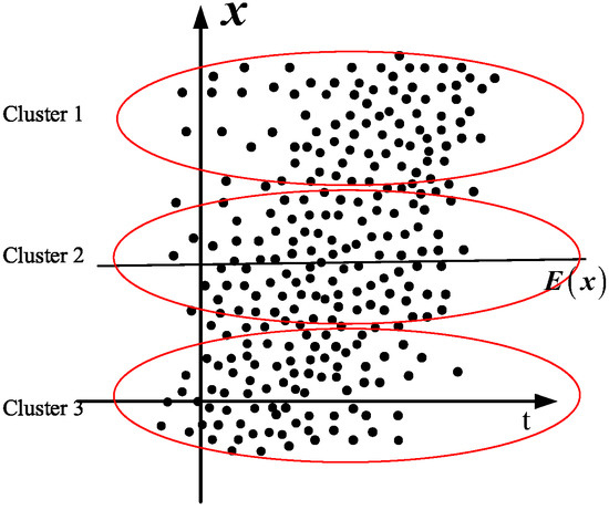
Figure 1.
Cluster results for static process.
As a result, the nearby points in Figure 1 (marked with red circles) have a close fluctuation, and hence, they are nearby points (clustered by KNN).
As shown in Figure 2, for the dynamic process the expectation is not fixed, and it changes over time, i.e., . In this situation, the Euclidean distance of the two sample values, and , is not equal to the Euclidean distance of the fluctuation at sample time and . In Figure 2a, the cluster result of nearby points based on the Euclidean distances of original variable values is wrong because it ignores the changing of , and hence, the data with close sample times are more likely to be clustered into one group. As the process goes on, the expectation values of the variables deviate a lot from those of the training data, and hence, the false alarm rate will be very large. In Figure 2b, the cluster result is right because each cluster consists of a data sample from a different sample time, and it is not influenced by the changing of the expectation value. As such, how to handle the changing expectation value is the key to addressing the dynamic process feature.
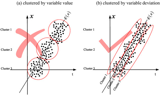
Figure 2.
Cluster results for dynamic static process: (a) clustered by variable value and (b) clustered by variable deviation.
3.2. New Two-Step Dynamic Scheme
To handle the dynamic issue, the key step is to extract the static components from the dynamic data. One drawback of the traditional two-step dynamic scheme is that and are related even if is very large, and hence, the dynamic matrix may be wrong. In this paper, we introduce another independent sample dataset as
and calculate the difference between two datasets as
where
is the component related to and is the static component which is independent of . As and follow the same statistical distribution, hence the expectation value of is zero and can be estimated with the least squares algorithm. The following steps are the same as in the traditional two-step dynamic scheme.
3.3. Two-Step Dynamic Local Kernel Principal Component Analysis (TSD-LKPCA)
As shown in Figure 3, one gets that the static components extracted from are independent of the changing variable expectation value, and hence, can be used for LKPCA.
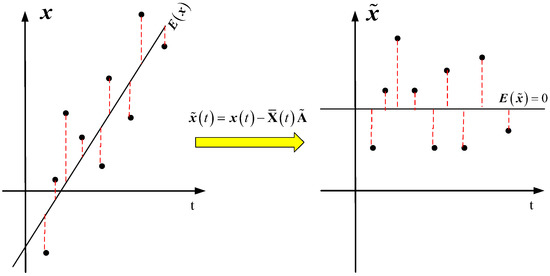
Figure 3.
Static components extracted from the dynamic process data.
The details of TSD-LKPCA are as follows.
Step 1. Process the original data with the new two-step dynamic scheme and extract the static components with Equation (13).
Step 2. Cluster into several nearby groups by using KNN and then calculate the neighborhood matrix by using Equation (7).
Step 3. Process with the kernel function and calculate the projection vector by using Equation (10).
Step 4. Extract the PCs by using Equation (6) and then monitor them by the and indices.
4. Simulation Results
In this section, we test the performance of TSD-LKPCA based on a numerically simulated dynamic nonlinear process and a TE process. The monitoring results acquired by this approach are compared to those obtained by PCA, KPCA, and LKPCA in terms of detection rate and false alarm rate.
4.1. Numerical Model Test
In order to verify the superiority of TSD-LKPCA in a dynamic nonlinear process, the following mathematical model is designed to test the effectiveness of the algorithm:
where is a random uniform distribution, , , are Gaussian random noise with zero mean and variance 0.01, and , , are the monitoring variables. This process generates 860 samples of normal data for off-line training and another 960 samples for testing. These test data introduce faults at the 450th sampling points.
There are two types of faults, as follows:
- Fault 1: a step fault occurs at variable with an amplitude of −6;
- Fault 2: the coefficient 0.8 in variable changes to 0.5.
For the three nonlinear approaches, KPCA, LKPCA, and TSD-LKPCA, the kernel width parameter is set to 50,000 by cross-validation. The LKPCA and TSD-LKPCA methods’ neighborhood relation parameter is 15. The dynamic process description model’s lag parameter is set to 2. The control limits for the four methods are based on a confidence limit of 99%. All these parameters are also used in the following Section 4.2.
Table 3 shows the false alarm rates and fault detection rates of four algorithms. Due to the nonlinear characteristics of the process, the average statistics of the false alarm rates of the three nonlinear methods, i.e., KPCA, LKPCA, and TSD-LKPCA, are much lower than that of the linear method PCA. Because KPCA and LKPCA are static methods, on the one hand they regard the change of expectation value in the training data as the normal data fluctuation, and hence, the control limits are very high in both methods, and they are insensitive to the faults; on the other hand, they regard the change of data expectation values in the testing data as the deviation caused by faults, resulting in large false detection. However, because TSD-LKPCA effectively handles the nonlinear and dynamic characteristics of the process, it achieves a 100% detection rate for both faults. The best result in each item is marked in underline and bold.
Table 3.
Monitoring results (%) of PCA, KPCA, LKPCA, and TSD-LKPCA.
The monitoring curves for faults 1 and 2 are depicted in Figure 4 and Figure 5. The blue line indicates the statistics, the red line represents the corresponding control limit, and the orange line represents the failure time in these two graphs. The statistics of PCA, KPCA, and LKPCA change over time in both figures, while the statistics of TSD-LKPCA do not change because it monitors the static components, whose expectation value is fixed. Because there is a deviation between the initial process dataset and the mean value of the training data, this deviation is regarded as a fault, and hence, the and statistics of the PCA, KPCA, and LKPCA algorithms initially exceeded the control limit, resulting in a false alarm. However, the TSD-LKPCA method has handled the dynamic characteristics and hence avoided this issue. For fault 1, as shown in Figure 4, when a fault occurs the PCA, KPCA, and LKPCA algorithms detect the fault after a period of time, which causes detection delay. For fault 2, as shown in Figure 5, the mean or variance of the statistics for the PCA, KPCA, and LKPCA methods change over time because of the dynamic feature, and hence, they are insensitive to the fault. In contrast, the TSD-LKPCA method detects the fault immediately, demonstrating that it has great sensitivity in fault detection in the process of nonlinear dynamic characteristics.
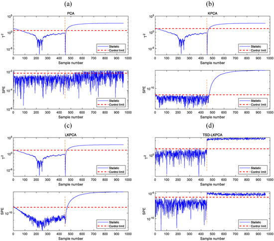
Figure 4.
Monitoring charts of fault 1 in the numerical example: (a) PCA, (b) KPCA, (c) LKPCA (d) TSD-LKPCA.
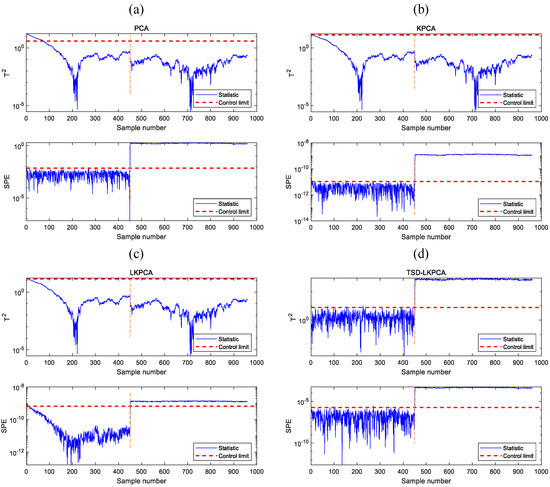
Figure 5.
Monitoring charts of fault 2 in the numerical example: (a) PCA, (b) KPCA, (c) LKPCA (d) TSD-LKPCA.
4.2. Tennessee Eastman (TE) Process Test
The Tennessee Eastman (TE) process is based on simulation models of actual industrial processes and is frequently used as a publicly available data source for testing process monitoring methods. The entire process system has 12 operational variables, 22 continuous variables, and 19 component variables. The training dataset consists of 960 normal data samples collected under normal operating circumstances. The TE process also produces 21 distinct types of faults (as shown in Table 4), which contain 960 samples of where the fault occurs, from the 161st data point to the end.
Table 4.
Fault descriptions for the Tennessee Eastman (TE) process.
As the TE process is a nonlinear and dynamic simulation model, it is, hence, adopted to test the performance of PCA, KPCA, LKPCA, and TSD-LKPCA. For method comparison, 315 samples of a normal process dataset were utilized for model training. Table 5 displays the detection results of 21 faults. Obviously, TSD-LKPCA achieves the best fault detection rate in 14 of the 21 faults and it has much lower false alarm rates than PCA and KPCA. In particular, TSD-LKPCA achieves a 100% fault detection rate in fault 5, and those of the other methods are lower than 45%. TSD-LKPCA also achieves much better than other the methods in faults 10, 16, 19, and 20. For fairness, we take the difference between the fault detection rates and the false alarm rates as an index, which indicates that TSD-LKPCA can achieve a much higher fault detection rate with the same false alarm rate. The best result in each item is marked in underline and bold.
Table 5.
Monitoring results on the TE process (%).
Figure 6 provides monitoring diagrams for several algorithms in fault 5. Fault 5 is the fault of a sudden change in the intake temperature of the cooling water, which occurs from the 161st data point to the end. According to the detection result curves of PCA (Figure 6a), KPCA (Figure 6b), and LKPCA (Figure 6c), the process is considered to have returned to normal after the 400th sample. In contrast, TSD-LKPCA (Figure 6d) still alarms the fault after that time, and hence, it achieves a 100% fault detection rate. This result also demonstrates that the TSD-LKPCA method outperforms PCA, KPCA, and LKPCA.
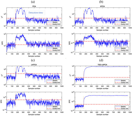
Figure 6.
Monitoring charts of fault 5: (a) PCA, (b) KPCA, (c) LKPCA (d) TSD-LKPCA.
5. Conclusions, Limitations, and Future Research
This paper proposed a TSD-LKPCA method for handling the dynamic and nonlinear features simultaneously. Our novel contribution proposes a novel two-step dynamic scheme and integrates it into the LKPCA technique naturally. As such, TSD-LKPCA can successfully extract the static component in the data and handle its nonlinear feature by LKPCA. The testing results in a dynamic and nonlinear numerical model show that TSD-LKPCA can successfully detect all types of faults, and the testing result in the TE process shows that TSD-LKPCA achieves a higher fault detection rate than PCA, KPCA, and LKPCA by more than 9%. As such, TSD-LKPCA is a promising method.
Another contribution of this paper is that it analyzed the influence of the dynamic feature on the clustering results of nearby points in detail and proved that LKPCA is not applicable to dynamic processes.
However, it is worth noting that the selection of parameter in the Gaussian kernel function and parameter in the KNN method is still a problem to be solved. More accurate results can be obtained by using more advanced parameter optimization methods. After some modifications, the algorithm for parameter optimization can be designed, which will be considered for future work.
Author Contributions
Conceptualization, H.F.; methodology, H.F. and Z.L.; validation, W.T. and S.L.; formal analysis, H.F.; resources, Y.W. and Y.X.; writing—original draft preparation, H.F.; writing—review and editing, Z.L. and W.T.; visualization, H.F. and W.T.; supervision, S.L.; project administration, Z.L.; funding acquisition, S.L., Z.L. and Y.X. All authors have read and agreed to the published version of the manuscript.
Funding
This work was supported by the Innovation Team of the Department of Education of Guangdong Province, China (2020KCXTD041), the School Level Scientific Research Project of SZPT, China (6022310005K), and Young Talents by the Department of Education of Guangdong Province, China (2021KQNCX210).
Conflicts of Interest
The authors declare no conflict of interest.
References
- Gao, Z.; Liu, X. An Overview on Fault Diagnosis, Prognosis and Resilient Control for Wind Turbine Systems. Processes 2021, 9, 300. [Google Scholar] [CrossRef]
- Aslam, M.; Bantan, R.A.R.; Khan, N. Monitoring the Process Based on Belief Statistic for Neutrosophic Gamma Distributed Product. Processes 2019, 7, 209. [Google Scholar] [CrossRef] [Green Version]
- Quiñones-Grueiro, M.; Prieto-Moreno, A.; Verde, C.; Llanes-Santiago, O. Data-driven monitoring of multimode continuous processes: A review. Chemom. Intell. Lab. Syst. 2019, 189, 56–71. [Google Scholar] [CrossRef]
- Qin, S.J. Survey on data-driven industrial process monitoring and diagnosis. Annu. Rev. Control 2012, 36, 220–234. [Google Scholar] [CrossRef]
- Abdi, H.; Williams, L.J. Principal component analysis. Wiley Interdiscip. Rev. Comput. Stat. 2010, 2, 433–459. [Google Scholar] [CrossRef]
- Zhou, P.; Zhang, R.; Xie, J.; Liu, J.; Wang, H.; Chai, T. Data-driven monitoring and diagnosing of abnormal furnace conditions in blast furnace ironmaking: An integrated PCA-ICA method. IEEE Trans. Ind. Electron. 2020, 68, 622–631. [Google Scholar] [CrossRef]
- Lou, Z.; Wang, Y.; Lu, S.; Sun, P. Process Monitoring Using a Novel Robust PCA Scheme. Ind. Eng. Chem. Res. 2021, 60, 4397–4404. [Google Scholar] [CrossRef]
- Song, Y.; Liu, J.; Zhang, L.; Wu, D. Improvement of Fast Kurtogram Combined with PCA for Multiple Weak Fault Features Extraction. Processes 2020, 8, 1059. [Google Scholar] [CrossRef]
- Lei, Y.; Jiang, W.; Jiang, A.; Zhu, Y.; Niu, H.; Zhang, S. Fault diagnosis method for hydraulic directional valves integrating PCA and XGBoost. Processes 2019, 7, 589. [Google Scholar] [CrossRef] [Green Version]
- Fu, Y.; Gao, Z.; Liu, Y.; Zhang, A.; Yin, X. Actuator and Sensor Fault Classification for Wind Turbine Systems Based on Fast Fourier Transform and Uncorrelated Multi-Linear Principal Component Analysis Techniques. Processes 2020, 8, 1066. [Google Scholar] [CrossRef]
- Kresta, J.V.; MacGregor, J.F.; Marlin, T.E. Multivariate statistical monitoring of process operating performance. Can. J. Chem. Eng. 1991, 69, 35–47. [Google Scholar] [CrossRef]
- Dong, J.; Zhang, K.; Huang, Y.; Li, G.; Peng, K. Adaptive total PLS based quality-relevant process monitoring with application to the Tennessee Eastman process. Neurocomputing 2015, 154, 77–85. [Google Scholar] [CrossRef]
- Kano, M.; Tanaka, S.; Hasebe, S.; Hashimoto, I.; Ohno, H. Monitoring independent components for fault detection. AIChE J. 2003, 49, 969–976. [Google Scholar] [CrossRef] [Green Version]
- Fan, J.; Qin, S.J.; Wang, Y. Online monitoring of nonlinear multivariate industrial processes using filtering KICA–PCA. Control Eng. Pract. 2014, 22, 205–216. [Google Scholar] [CrossRef]
- Cartocci, N.; Napolitano, M.R.; Crocetti, F.; Costante, G.; Valigi, P.; Fravolini, M.L. Data-Driven Fault Diagnosis Techniques: Non-Linear Directional Residual vs. Machine-Learning-Based Methods. Sensors 2022, 22, 2635. [Google Scholar] [CrossRef]
- Dunia, R.; Qin, S.J. Joint diagnosis of process and sensor faults using principal component analysis. Control Eng. Pract. 1998, 6, 457–469. [Google Scholar] [CrossRef]
- Lee, J.-M.; Yoo, C.; Choi, S.W.; Vanrolleghem, P.A.; Lee, I.-B. Nonlinear process monitoring using kernel principal component analysis. Chem. Eng. Sci. 2004, 59, 223–234. [Google Scholar] [CrossRef]
- Jiang, Q.; Yan, X. Parallel PCA–KPCA for nonlinear process monitoring. Control Eng. Pract. 2018, 80, 17–25. [Google Scholar] [CrossRef]
- Zhang, Y. Enhanced statistical analysis of nonlinear processes using KPCA, KICA and SVM. Chem. Eng. Sci. 2009, 64, 801–811. [Google Scholar] [CrossRef]
- Zeng, L.; Long, W.; Li, Y. A Novel Method for Gas Turbine Condition Monitoring Based on KPCA and Analysis of Statistics T2 and SPE. Processes 2019, 7, 124. [Google Scholar] [CrossRef] [Green Version]
- Zhou, M.; Zhang, Q.; Liu, Y.; Sun, X.; Cai, Y.; Pan, H. An Integration Method Using Kernel Principal Component Analysis and Cascade Support Vector Data Description for Pipeline Leak Detection with Multiple Operating Modes. Processes 2019, 7, 648. [Google Scholar] [CrossRef] [Green Version]
- Wang, Y.; Si, Y.; Huang, B.; Lou, Z. Survey on the theoretical research and engineering applications of multivariate statistics process monitoring algorithms: 2008–2017. Can. J. Chem. Eng. 2018, 96, 2073–2085. [Google Scholar] [CrossRef]
- Lahdhiri, H.; Elaissi, I.; Taouali, O.; Harakat, M.F.; Messaoud, H. Nonlinear process monitoring based on new reduced Rank-KPCA method. Stoch. Environ. Res. Risk Assess. 2018, 32, 1833–1848. [Google Scholar] [CrossRef]
- Peng, G.; Huang, K.; Wang, H. Dynamic multimode process monitoring using recursive GMM and KPCA in a hot rolling mill process. Syst. Sci. Control Eng. 2021, 9, 592–601. [Google Scholar] [CrossRef]
- Deng, X.; Tian, X.; Chen, S. Modified kernel principal component analysis based on local structure analysis and its application to nonlinear process fault diagnosis. Chemom. Intell. Lab. Syst. 2013, 127, 195–209. [Google Scholar] [CrossRef] [Green Version]
- Parra, L.; Sajda, P. Blind source separation via generalized eigenvalue decomposition. J. Mach. Learn. Res. 2003, 4, 1261–1269. [Google Scholar]
- Kramer, O. K-nearest neighbors. In Dimensionality Reduction with Unsupervised Nearest Neighbors; Springer: Berlin/Heidelberg, Germany, 2013; pp. 13–23. [Google Scholar]
- Wang, J.; Zhou, Z.; Li, Z.; Du, S. A Novel Fault Detection Scheme Based on Mutual k-Nearest Neighbor Method: Application on the Industrial Processes with Outliers. Processes 2022, 10, 497. [Google Scholar] [CrossRef]
- Lou, Z.; Tuo, J.; Wang, Y. Two-step principal component analysis for dynamic processes. In Proceedings of the 2017 6th International Symposium on Advanced Control of Industrial Processes (AdCONIP), Taipei, Taiwan, 28–31 May 2017; pp. 73–77. [Google Scholar]
- Lou, Z.; Wang, Y.; Si, Y.; Lu, S. A novel multivariate statistical process monitoring algorithm: Orthonormal subspace analysis. Automatica 2022, 138, 110148. [Google Scholar] [CrossRef]
- Chiang, L.H.; Russell, E.L.; Braatz, R.D. Fault Detection and Diagnosis in Industrial Systems; Springer Science & Business Media: Berlin/Heidelberg, Germany, 2000. [Google Scholar]
- Xu, Y.; Zhang, D.; Song, F.; Yang, J.-Y.; Jing, Z.; Li, M. A method for speeding up feature extraction based on KPCA. Neurocomputing 2007, 70, 1056–1061. [Google Scholar] [CrossRef]
- Lou, Z.; Shen, D.; Wang, Y. Preliminary-summation-based principal component analysis for non-Gaussian processes. Chemom. Intell. Lab. Syst. 2015, 146, 270–289. [Google Scholar] [CrossRef]
- Deng, X.; Cai, P.; Cao, Y.; Wang, P. Two-step localized kernel principal component analysis based incipient fault diagnosis for nonlinear industrial processes. Ind. Eng. Chem. Res. 2020, 59, 5956–5968. [Google Scholar] [CrossRef]
- Lou, Z.; Shen, D.; Wang, Y. Two-step principal component analysis for dynamic processes monitoring. Can. J. Chem. Eng. 2018, 96, 160–170. [Google Scholar] [CrossRef]
- Han, M.; Zhang, S.; Xu, M.; Qiu, T.; Wang, N. Multivariate chaotic time series online prediction based on improved kernel recursive least squares algorithm. IEEE Trans. Cybern. 2018, 49, 1160–1172. [Google Scholar] [CrossRef] [PubMed]
- Ma, X.; Si, Y.; Yuan, Z.; Qin, Y.; Wang, Y. Multistep dynamic slow feature analysis for industrial process monitoring. IEEE Trans. Instrum. Meas. 2020, 69, 9535–9548. [Google Scholar] [CrossRef]
- Cong, Y.; Zhou, L.; Song, Z.; Ge, Z. Multirate dynamic process monitoring based on multirate linear Gaussian state-space model. IEEE Trans. Autom. Sci. Eng. 2019, 16, 1708–1719. [Google Scholar] [CrossRef]
Publisher’s Note: MDPI stays neutral with regard to jurisdictional claims in published maps and institutional affiliations. |
© 2022 by the authors. Licensee MDPI, Basel, Switzerland. This article is an open access article distributed under the terms and conditions of the Creative Commons Attribution (CC BY) license (https://creativecommons.org/licenses/by/4.0/).