Detection and Isolation of Incipiently Developing Fault Using Wasserstein Distance

Abstract

This paper develops an incipient fault detection and isolation method using the Wasserstein distance, which measures the difference between the probability distributions of normal and faulty data sets from the aspect of optimal transport. For fault detection, a moving window based approach is introduced, resulting in two monitoring statistics that are constructed based on the Wasserstein distance. From analysis of the limiting distribution under multivariate Gaussian case, it is proved that the difference measured by the Wasserstein distance is more sensitive than conventional quadratic statistics like Hotelling’s $T^2$ and Squared Prediction Error (SPE). For non-Gaussian distributed data, a project robust Wasserstein distance (PRW) model is proposed and the Riemannian block coordinate descent (RBCD) algorithm is applied to estimate the Wasserstein distance, which is fast when the number of sampled data is large. In addition, a fault isolation method is further proposed once the incipiently developing fault is detected. Application studies to a simulation example, a continuous stirred tank reactor (CSTR) process and a real-time boiler water wall over-temperature process demonstrate the effectiveness of the proposed method.

1. Introduction

Process monitoring plays a significant role in improving the reliability and safety of modern industrial systems. With the advancement of information and sensor technology, data collection has become more convenient and data processing has become more rapid, which greatly facilitates the developing of data-driven process monitoring methods. Compared with model-based monitoring methods, data-driven technology does not require much prior knowledge, is conceptually simple, and has low implementation costs [1]. Among different kinds of data-driven methods, the most popular is perhaps multivariate statistical based approaches [2], typical analysis methods include principal component analysis (PCA) [3], independent principal component analysis (ICA) [4], and Fisher discriminant analysis (FDA) [5]. The basic idea of multivariate statistical methods is to map the process data onto a low-dimensional space through a specific transformation to obtain latent variables, and construct monitoring statistics like Hotelling’s $T^2$ and squared prediction error (SPE) to determine whether the process data is faulty [6]. Based on multivariate statistical methods, the literature have proposed a series of techniques for monitoring of different kinds of fault types like distributed faults [7], intermittent faults [8], and incipient faults [9].

In recent years, detection of incipiently developing faults has attracted significant research attention, as it is of great benefits for industrial operators to detect and correct an incipient fault at an early stage. A number of techniques have been developed for monitoring of incipient faults, which roughly falls into three categories, namely, methods based on higher-order information, smoothing and denoising based approaches and statistical distance based approaches. Methods based on higher-order information considers the incorporation of higher-order information in the monitoring statistics to cope with incipient faults, including those based on recursive correlative statistical analysis [10], statistical local approach [11], and recursive transform component analysis [12].

The second type of approaches use smoothing and denoising techniques to remove noises and disturbances to enhance the detection sensitivity for incipient faults, such as detrending and denoising based method [13], smoothing based method [14] and non-stationary analysis [15]. Last but not least, statistical distance based approaches use statistical measures that are regarded to be sensitive to small disturbances to perform incipient fault detection. The most widely used statistical distance for incipient fault detection is the Kullback Leibler divergence(KLD). For instance, Harmouche et al. proposed a monitoring method based on KLD under the PCA framework [16], Zeng et al. [9] analyzed the theoretical properties of KLD and proved that KLD is more sensitive than conventional quadratic monitoring statistics, some variants of the KLD have also been developed to accommodate more complicated situations [17,18,19]. Besides, other statistical distances have also been used, such as Jensen-Shannon divergence [20] and Mahalanobis distance [21,22]. To cope with the incipient fault isolation problem, several methods are also proposed, such as probabilistic amplitude estimation method in the framework of KLD [23] and exponential smoothing reconstruction [24]. Deep learning is another very effective method of fault isolation, in which autoencoders and recurrent neural networks have been widely used in process monitoring. In recent work, an improved autoencoder based on sliding-scale resampling strategy is proposed by Yang et al. [25] to isolate incipient fault, Jana et al. [26] proposed convolutional neural networks(CNN) and convolutional autoencoder (CAE) end-to-end framework to reconstructed fault, Sun et al. [27] utilized Bayesian Recurrent Neural Networks (BRNN) with variational dropout for fault detection and combined squared Mahalanobis distance and local density ratio (LDR) to identify Gaussian and non-Gaussian distributed fault variables, respectively.

Despite the research progress on incipient fault detection and isolation, some important issues still remain. First, the recursive methods based on higher-order information [10,11] required to monitor the mass variables at the same time, but some of them cannot be directly obtained; Second, existing method of smoothing techniques [14] improved the detection performance at the cost of detection timeliness, which is not suitable for online monitoring. As for Harmouche et al. [16] and Zeng et al. [9] calculated KLD under the PCA framework, they did not propose effective fault isolation methods. Though Harmouche et al. [23] estimated KLD by a probabilistic way, since KLD has no closed form, the magnitudes of the fault are approximate. Also, the statistical distance method based on Mahalanobis distance [21,22] are calculated by the covariance matrix of the reference data, which is highly demanding on the reference dataset. With regard to deep learning method [25,26,27], they can be effective when there are large number of training sets. However, they may suffer from heavy computation load and are difficult to get sparse fault isolation results.

Motivated by the above discussion, this paper proposes a new incipient fault detection and isolation method based on the Wasserstein distance [28] in the multivariate statical analysis framework, the three main contributions of this article are (1) a novel monitoring approach based on Wasserstein distance with sliding window is developed to detect incipient faults, the limiting distribution and sensitivity analysis of Wasserstein distance are discussed; (2) by introducing the Riemannian block coordinate descent algorithm [29] for estimation of the Wasserstein distance under the non-Gaussian case, an efficient detection method that is suitable for online application is proposed; (3) a fault isolation method based on the Wasserstein distance is designed, resulting in a complete fault detection and isolation framework of incipient faults.

This paper is organized as follows. Section 2, introduced the Wasserstein distance and some of its statistical characteristics as monitoring statistic. The monitoring method of Wasserstein distance of multivariate normal distribution data is studied in Section 3, and we also analyze the sensitivity of Wasserstein distance and Hotelling’s $T^2$ statistics. Section 4, a Wasserstein distance monitoring method for non-Gaussian distributed process data is designed. A fault isolation method based on Wasserstein distance is proposed in Section 5. In Section 6, the proposed method is applied to a simulate example and an industrial boiler that involves an over-temperature fault in the water-wall tube, the effectiveness of the method is proved. The conclusions of this work are presented in Section 7.

2. Preliminaries

This section presents preliminary knowledge involving multivariate statistical based process monitoring framework, the definition of Wasserstein distance and its limiting distribution under multivariate Gaussian case.

2.1. Multivariate Statistical Based Process Monitoring Framework

Assume m measurements of $d_x$ correlated variables $\mathbf{x}\in {\mathbb{R}}^{d_x}$ have been collected under normal conditions from the process and arranged into a data matrix $\mathbf{X}=\left\{{\mathbf{x}}_i,i=1,\cdots ,m\right\}$, ${\mathbf{x}}_i\in {\mathbb{R}}^{d_x}$. In the multivariate statistical based monitoring framework, the data matrix $\mathbf{X}$ is often used as a training data set and the following model structure is generally considered.

$$\mathbf{x}=\mathbf{Az}+\mathbf{e}$$

(1)

Here $\mathbf{z}={\mathbf{w}}^T\mathbf{x}$ is the $d(d\le d_x)$ dimensional score vector in the projection subspace, $\mathbf{e}=(\mathbf{I}-{\mathbf{Aw}}^T)\mathbf{x}$ is the residual vector, with $\mathbf{w}\in {\mathbb{R}}^{d_x\times d}$ being the projection matrix, $\mathbf{A}\in {\mathbb{R}}^{d_x\times d}$ being the loading matrix and $\mathbf{I}$ being the identity matrix. The projection matrix can be estimated using different techniques, such as principal component analysis, independent component analysis or canonical correlation analysis. On the other hand, another set of n measurements are also collected and arranged as $\tilde{\mathbf{X}}=\left\{{\tilde{\mathbf{x}}}_k,k=1,\cdots ,n\right\}$, ${\tilde{\mathbf{x}}}_k\in {\mathbb{R}}^{d_x}$, which is generally used as the test data set. Similar to Equation (1), the model structure for the test data set can be constructed as follows.

$$\tilde{\mathbf{x}}=\mathbf{A}\tilde{\mathbf{z}}+\tilde{\mathbf{e}}$$

(2)

Here $\tilde{\mathbf{z}}\in {\mathbb{R}}^d$ is the score vector and $\tilde{\mathbf{e}}\in {\mathbb{R}}^{d_x}$ the residual vector. The purpose of process monitoring is to investigate whether the score vectors $\mathbf{z}$ and $\tilde{\mathbf{z}}$, as well as the residual vectors $\mathbf{e}$ and $\tilde{\mathbf{e}}$, share the same distribution. This can be achieved by constructing quadratic statistics like Hotelling’s $T^2$ or SPE, which can be defined as follows.

$$\begin{array}{c}{T}^2={\mathbf{z}}^T\mathbf{z}={\mathbf{x}}^T{\mathbf{ww}}^T\mathbf{x}\\ \mathrm{SPE}={\mathbf{e}}^{\mathrm{T}}\mathbf{e}={\mathbf{x}}^{\mathrm{T}}{(\mathbf{I}-{\mathbf{AW}}^{\mathrm{T}})}^{\mathrm{T}}(\mathbf{I}-{\mathbf{AW}}^{\mathrm{T}})\mathbf{x}\end{array}$$

(3)

The control limits of the quadratic statistics can be obtained based on the normal samples using statistical analysis. For a specific sample in the test data set, the corresponding statistics can be constructed similar to Equation (3), violation of the control limits of either statistic indicates that a faulty condition arises. Such quadratic statistics, however, have been shown to be not sensitive enough for incipiently developing fault conditions [9]. Instead, the Wasserstein distance is considered alternatively in this paper.

2.2. Definition of Wasserstein Distance

Wasserstein distance is a distance function used to measure the difference between probability distributions [30]. The Wasserstein distance arises from the optimal transportation theory and can be regarded as the minimum cost of transporting when converting one distribution to another. Due to its conceptual simplicity, it has seen a wide range of applications in probability theory, statistics and machine learning [28,31]. Let $\mathbf{z}$ and $\tilde{\mathbf{z}}$ be d-dimensional random vectors from a normed vector space $(\chi ,\parallel ·\parallel )$, with $\parallel ·\parallel$ being the underlying norm, f and $\tilde{f}$ being two probability measures, $\mathbf{z}\sim f$ and $\tilde{\mathbf{z}}\sim \tilde{f}$. The p-Wasserstein distance($p\ge 1$) between $\mathbf{z}$ and $\tilde{\mathbf{z}}$ can be defined as follows [32].

$${\mathcal{W}}_p\left(f,\tilde{f}\right)=\underset{\mathbf{\pi }\in \mathsf{\Pi }\left(f,\tilde{f}\right)}{inf}{\left({\int }_{\chi \times \chi }{∥\mathbf{z}-\tilde{\mathbf{z}}∥}^{p}d\mathbf{\pi }\left(\mathbf{z},\tilde{\mathbf{z}}\right)\right)}^{1/p}$$

(4)

Here, $\mathsf{\Pi }\left(f,\tilde{f}\right)$ is the set of probability measures $\mathbf{\pi }$ on $\chi \times \chi$, whose marginal distributions are f and $\tilde{f}$, respectively. For practical application, the underlying norm $\parallel ·\parallel$ is generally set as Euclidean norm. In addition, $p=2$ is always considered and ${∥\mathbf{z}-\tilde{\mathbf{z}}∥}^p$ becomes the Euclidean distance.

2.3. Limit Distribution of Wasserstein Distance under Multivariate Gaussian Case

In order to be used as a monitoring statistic, the limit distribution of Wasserstein distance should be determined, so that the control limit can be obtained by analyzing its limit distribution. Assume $\mathbf{z}$ and $\tilde{\mathbf{z}}$ follow multivariate Gaussian distributions, with $f=\mathcal{N}\left({\mathbf{\mu }}_1,{\mathsf{\Sigma }}_1\right)$, $\tilde{f}=\mathcal{N}\left({\mathbf{\mu }}_2,{\mathsf{\Sigma }}_2\right)$, ${\mathbf{\mu }}_1,{\mathbf{\mu }}_2\in {\mathbb{R}}^d$ being the mean vectors and ${\mathsf{\Sigma }}_1,{\mathsf{\Sigma }}_2\in {\mathbb{R}}^{d\times d}$ being symmetric, positive covariance matrices. The following Lemma holds.

Lemma 1.

The Wasserstein distance between f and $\tilde{f}$ can be computed as follows [33].

$${\mathcal{W}}^2(f,\tilde{f})={∥{\mathbf{\mu }}_1-{\mathbf{\mu }}_2∥}^2+\mathrm{tr}\left({\mathsf{\Sigma }}_1\right)+\mathrm{tr}\left({\mathsf{\Sigma }}_2\right)-2\mathrm{tr}\left({\left({\mathsf{\Sigma }}_1^{1/2}{\mathsf{\Sigma }}_2{\mathsf{\Sigma }}_1^{1/2}\right)}^{1/2}\right)$$

(5)

Here, $\mathrm{tr}\left(·\right)$ denotes the trace of a matrix, $\parallel ·\parallel$ denotes the Euclidean norm.

In order to obtain the limit distribution, it is assumed that the probability density function(PDF) f of $\mathbf{z}$ is known a priori. In contrast, the density of $\tilde{\mathbf{z}}$ is estimated from a data set $\tilde{\mathbf{z}}=\{{\tilde{\mathbf{z}}}_k,k=1,\cdots ,n\}$ and denoted as $\widehat{\tilde{f}}$, with ${\tilde{\mathbf{z}}}_k\in {\mathbb{R}}^d$ being the k-th i.i.d data point sampled from $\tilde{f}$. Based on $\tilde{\mathbf{z}}$, the empirical mean vector and empirical covariance matrix can be calculated as follows.

$$\begin{array}{c}{\widehat{\mathbf{\mu }}}_2=\frac{1}{n}{\displaystyle \sum _{k=1}^n}{\tilde{\mathbf{z}}}_k\\ {\widehat{\mathsf{\Sigma }}}_2=\frac{1}{n-1}{\displaystyle \sum _{k=1}^n}\left({\tilde{\mathbf{z}}}_k-{\widehat{\mathbf{\mu }}}_2\right){\left({\tilde{\mathbf{z}}}_k-{\widehat{\mathbf{\mu }}}_2\right)}^T\end{array}$$

(6)

The Wasserstein distance between f and $\widehat{\tilde{f}}$ can be obtained as

$${\widehat{\mathcal{W}}}^2={\mathcal{W}}^2(f,\widehat{\tilde{f}})={\mathcal{W}}^2\left(\mathcal{N}({\mathbf{\mu }}_1,{\mathsf{\Sigma }}_1),\mathcal{N}({\widehat{\mathbf{\mu }}}_2,{\widehat{\mathsf{\Sigma }}}_2)\right)$$

(7)

For the purpose of clarity, ${\widehat{\mathcal{W}}}^2$ is called the empirical Wasserstein distance and ${\mathcal{W}}^2$ the true Wasserstein distance. Theorem 1 shows that the square of difference between empirical and true Wasserstein distance follows a scaled ${\chi }^2$ distribution [34].

Theorem 1.

Let $\mathbf{z}$ and $\tilde{\mathbf{z}}$ be two Gaussian distributed random vectors with probability measures $f=\mathcal{N}\left({\mathbf{\mu }}_1,{\mathsf{\Sigma }}_1\right)$ and $\tilde{f}=\mathcal{N}\left({\mathbf{\mu }}_2,{\mathsf{\Sigma }}_2\right)$, ${\mathbf{\mu }}_1\ne {\mathbf{\mu }}_2$ or ${\mathsf{\Sigma }}_1\ne {\mathsf{\Sigma }}_2$, $\widehat{\tilde{f}}=\mathcal{N}\left(\widehat{{\mathbf{\mu }}_2},{\widehat{\mathsf{\Sigma }}}_2\right)$ be the empirical density of $\tilde{f}$ estimated from Equation (4), the square of difference between empirical and true Wasserstein distance follows a scaled ${\chi }^2$ distribution as $n\to \infty$.

$$\mathbb{W}=\frac{n}{{\omega }^2}{\left({\widehat{\mathcal{W}}}^2-{\mathcal{W}}^2\right)}^2\Rightarrow {\chi }_1^2$$

(8)

With

$$\begin{array}{c}{\omega }^2=4{\left({\mathbf{\mu }}_1-{\mathbf{\mu }}_2\right)}^T{\mathsf{\Sigma }}_2\left({\mathbf{\mu }}_1-{\mathbf{\mu }}_2\right)+2\mathrm{tr}\left({\mathsf{\Sigma }}_2^2\right)+2\mathrm{tr}\left({\mathsf{\Sigma }}_1{\mathsf{\Sigma }}_2\right)\\ -4{\displaystyle \sum _{l=1}^d}{\kappa }_l^{1/2}{\mathbf{q}}_l^T{\mathsf{\Sigma }}_1^{-1/2}{\mathsf{\Sigma }}_2{\mathsf{\Sigma }}_1^{-1/2}{\mathbf{q}}_l\end{array}$$

(9)

Here ⇒ denotes the convergence of the distribution, $\left\{\left({\kappa }_l,{\mathbf{q}}_l\right):l=1,\cdots ,d\right\}$ denotes the eigendecomposition of the symmetric matrix ${\mathsf{\Sigma }}_1^{1/2}{\mathsf{\Sigma }}_2{\mathsf{\Sigma }}_1^{1/2}$.

Proof. 

For multivariate Gaussian distributed data sets, The empirical mean and empirical covariance are related to their true values as follows,

$$\begin{array}{c}\hfill \sqrt{n}\left({\widehat{\mathbf{\mu }}}_2-{\mathbf{\mu }}_2\right)\Rightarrow \mathbf{g}\end{array}$$

(10a)

$$\begin{array}{c}\hfill \sqrt{n}\left({\widehat{\mathsf{\Sigma }}}_2-{\mathsf{\Sigma }}_2\right)\Rightarrow \mathbf{G}\end{array}$$

(10b)

where $\mathbf{g}$∼$\mathcal{N}(\mathbf{0},{\mathsf{\Sigma }}_2)$ and $\mathbf{G}={{\mathsf{\Sigma }}_2}^{1/2}\mathbf{H}{{\mathsf{\Sigma }}_2}^{1/2}$ [35]. Here, convergence in the space ${\mathbb{R}}^d\times {\mathbb{R}}^{d\times d}$ is understood component wise and $\mathbf{H}={\left({\mathbf{H}}_{l_1,l_2}\right)}_{l_1.l_2\le d}$ is a symmetric random matrix with independent (upper triangular) entries as

$${\mathbf{H}}_{l_1,l_2}\sim \left\{\begin{array}{cc}\hfill & \mathcal{N}(0,1),l_1<l_2\hfill \\ \hfill & \mathcal{N}(0,2),l_1=l_2\hfill \end{array}\right.$$

(11)

Let the mapping of Wasserstein distance of multivariate Gaussian distribution $\varphi$ be given by

$$\varphi \left({\mathbf{\mu }}_1,{\mathbf{\mu }}_2,{\mathsf{\Sigma }}_1,{\mathsf{\Sigma }}_2\right)\mapsto {∥{\mathbf{\mu }}_1-{\mathbf{\mu }}_2∥}^2+tr\left({\mathsf{\Sigma }}_1\right)+tr\left({\mathsf{\Sigma }}_2\right)-2tr\left({\left({\mathsf{\Sigma }}_1^{1/2}{\mathsf{\Sigma }}_2{\mathsf{\Sigma }}_1^{1/2}\right)}^{1/2}\right)$$

(12)

For $\mathbf{g}$ and $\mathbf{G}$ discussed in Equation (11), by fixing ${\mathbf{\mu }}_1$ and ${\mathsf{\Sigma }}_1$, $\varphi$ is Frechet differentiable and its derivative at any point $\left({\mathbf{\mu }}_2,{\mathsf{\Sigma }}_2\right)$ is given as follows.

$$D_{({\mathbf{\mu }}_2,{\mathsf{\Sigma }}_2)}{\varphi }^{({\mathbf{\mu }}_1,{\mathsf{\Sigma }}_1)}\left[(\mathbf{g},\mathbf{G})\right]=2({\mathbf{\mu }}_2-{\mathbf{\mu }}_1)\mathbf{g}+tr\left(\mathbf{G}\right)-\sum _{l=1}^d{\kappa }_l^{-1/2}{\mathbf{q}}_l^T\sqrt{{\mathsf{\Sigma }}_1}\mathbf{G}\sqrt{{\mathsf{\Sigma }}_1}{\mathbf{q}}_l$$

(13)

Based on the delta method [36], the following asymptotic relationship can be obtained:

$$\sqrt{n}\left(\varphi \left({\mathbf{\mu }}_1,{\widehat{\mathbf{\mu }}}_2,{\mathsf{\Sigma }}_1,{\widehat{\mathsf{\Sigma }}}_2\right)-{\mathcal{W}}^2\left(f,\tilde{f}\right)\right)\Rightarrow D_{({\mathbf{\mu }}_2,{\mathsf{\Sigma }}_2)}{\varphi }^{({\mathbf{\mu }}_1,{\mathsf{\Sigma }}_1)}\left[\left(\mathbf{g},\mathbf{G}\right)\right]$$

(14)

It should be noticed that $\mathbf{H}$ has independent Gaussian entries in the upper triangle with mean 0 and variance 1 off-diagonal and variance 2 on the diagonal, the mean of $\mathbf{g}$ and $\mathbf{G}$ are both 0, thus, $D_{({\mathbf{\mu }}_2,{\mathsf{\Sigma }}_2)}{\varphi }^{({\mathbf{\mu }}_1,{\mathsf{\Sigma }}_1)}\left[\left(\mathbf{g},\mathbf{G}\right)\right]$ is a real-valued Gaussian variable with mean 0 and a certain variance $\omega$, and the scaled ${\chi }^2$ distribution is described as,

$$\frac{n}{{\omega }^2}{\left(\varphi \left({\mathbf{\mu }}_1,{\widehat{\mathbf{\mu }}}_2,{\mathsf{\Sigma }}_1,{\widehat{\mathsf{\Sigma }}}_2\right)-{\mathcal{W}}^2\left(f,\tilde{f}\right)\right)}^2\Rightarrow {\chi }_1^2$$

(15)

Now, we calculate the variance of the derivative in Equation (13), the first term of Equation (13) involving the means ${\mathbf{\mu }}_1$ and ${\mathbf{\mu }}_2$ is computed as follow,

$$\left({\mathbf{\mu }}_2-{\mathbf{\mu }}_1\right)\mathbf{g}\sim \mathcal{N}\left(0,{\left({\mathbf{\mu }}_2-{\mathbf{\mu }}_1\right)}^T{\mathsf{\Sigma }}_2\left({\mathbf{\mu }}_2-{\mathbf{\mu }}_1\right)\right)$$

(16)

The remaining terms involving the covariance matrices ${\mathsf{\Sigma }}_2$ in Equation (13) are given by,

$$\begin{array}{cc}\hfill & tr\left(\mathbf{G}\right)-\sum _{l=1}^d{\kappa }_l^{-1/2}{\mathbf{q}}_l^T{\mathsf{\Sigma }}_2^{1/2}\mathbf{G}{\mathsf{\Sigma }}_1^{1/2}{\mathbf{q}}_l\hfill \\ \hfill & =tr\left({\mathsf{\Sigma }}_2\mathbf{H}\right)-\sum _{l=1}^d{\kappa }_l^{-1/2}{\mathbf{q}}_l^T{\mathsf{\Sigma }}_1^{1/2}{\mathsf{\Sigma }}_2^{1/2}\mathbf{H}{\mathsf{\Sigma }}_2^{1/2}{\mathsf{\Sigma }}_1^{1/2}{\mathbf{q}}_l\hfill \end{array}$$

(17)

With this we can calculate the second moment and the variance of the centered Gaussian of Equation (17)

$$\begin{array}{cc}\hfill & E\left[{\left(tr\left({\mathsf{\Sigma }}_2\mathbf{H}\right)-\sum _{l=1}^d{\kappa }_l^{-1/2}{\mathbf{q}}_l^T{\mathsf{\Sigma }}_1^{1/2}\mathbf{G}{\mathsf{\Sigma }}_1^{1/2}{\mathbf{q}}_l\right)}^2\right]\hfill \\ \hfill & =\sum _{l_1,l_2=1}^d\left(E\left[{\mathbf{q}}_{l_1}^T{\mathsf{\Sigma }}_2\mathbf{H}{\mathbf{q}}_{l_1}{\mathbf{q}}_{l_2}^T{\mathsf{\Sigma }}_2\mathbf{H}{\mathbf{q}}_{l_2}\right]\right.\hfill \\ \hfill & +E\left[{\kappa }_{l_1}^{-1/2}{\kappa }_{l_2}^{-1/2}{\mathbf{q}}_{l_1}^T{\mathsf{\Sigma }}_1^{1/2}{\mathsf{\Sigma }}_2^{1/2}\mathbf{H}{\mathsf{\Sigma }}_2^{1/2}{\mathsf{\Sigma }}_1^{1/2}{\mathbf{q}}_{l_1}{\mathbf{q}}_{l_2}^T{\mathsf{\Sigma }}_1^{1/2}{\mathsf{\Sigma }}_2^{1/2}\mathbf{H}{\mathsf{\Sigma }}_2^{1/2}{\mathsf{\Sigma }}_1^{1/2}{\mathbf{q}}_{l_2}\right]\hfill \\ \hfill & \left.-2E\left[{\kappa }_{l_1}^{-1/2}{\mathbf{q}}_{l_2}^T{\mathsf{\Sigma }}_2\mathbf{H}{\mathbf{q}}_{l_2}{\mathbf{q}}_{l_1}^T{\mathsf{\Sigma }}_1^{1/2}{\mathsf{\Sigma }}_2^{1/2}\mathbf{H}{\mathsf{\Sigma }}_2^{1/2}{\mathsf{\Sigma }}_1^{1/2}{\mathbf{q}}_{l_1}\right]\right)\hfill \end{array}$$

(18)

The first term in Equation (18) can be rewritten as

$$\begin{array}{cc}\hfill & \sum _{l_1,l_2=1}^d\left({\mathbf{q}}_{l_1}^T{\mathsf{\Sigma }}_2{\left({\mathbf{q}}_{l_1}{\mathbf{q}}_{l_2}^T{\mathsf{\Sigma }}_2\right)}^T{\mathbf{q}}_{l_2}+{\mathbf{q}}_{l_1}^T{\mathsf{\Sigma }}_2{\mathbf{q}}_{l_2}tr\left({\mathbf{q}}_{l_1}{\mathbf{q}}_{l_2}^T{\mathsf{\Sigma }}_2\right)\right)\hfill \\ \hfill & =\sum _{l_1=1}^d{\mathbf{q}}_{l_1}^T{\mathsf{\Sigma }}_2^2{\mathbf{q}}_{l_1}+\sum _{l_1,l_2=1}^d{\mathbf{q}}_{l_1}^T{\mathsf{\Sigma }}_2{\mathbf{q}}_{l_2}{\mathbf{q}}_{l_2}^T{\mathsf{\Sigma }}_2{\mathbf{q}}_{l_1}\hfill \\ \hfill & =2\sum _{l=1}^d{\mathbf{q}}_l^T{\mathsf{\Sigma }}_2^2{\mathbf{q}}_l=2tr\left({\mathsf{\Sigma }}_2^2\right)\hfill \end{array}$$

(19)

Similar derivations can be used for the second and third terms in Equation (18) to obtain $2tr\left({\mathsf{\Sigma }}_1{\mathsf{\Sigma }}_2\right)$ and $-4{\displaystyle \sum _l^d}{\kappa }_l^{1/2}{\mathbf{q}}_l^T{\mathsf{\Sigma }}_1^{-1/2}{\mathsf{\Sigma }}_2{\mathsf{\Sigma }}_1^{1/2}{\mathbf{q}}_l$, respectively. Thus, ${\omega }^2$ can be described as follows,

$${\omega }^2=4{\left({\mathbf{\mu }}_2-{\mathbf{\mu }}_1\right)}^T{\mathsf{\Sigma }}_2\left({\mathbf{\mu }}_2-{\mathbf{\mu }}_1\right)+2tr\left({\mathsf{\Sigma }}_2^2\right)+2tr\left({\mathsf{\Sigma }}_1{\mathsf{\Sigma }}_2\right)-4\sum _{l=1}^d{\kappa }_l^{1/2}{\mathbf{q}}_l^T{\mathsf{\Sigma }}_1^{-1/2}{\mathsf{\Sigma }}_2{\mathsf{\Sigma }}_1^{1/2}{\mathbf{q}}_l$$

(20)

3. Wasserstein Distance as a Process Monitoring Statistic

Section 2.3 shows that the distribution of the square of difference between empirical and true Wasserstein distance is a scaled ${\chi }^2$ distribution. Hence $\mathbb{W}$ in Equation (8) can be used as a monitoring statistic to determine whether a set of sample share the same distribution as the reference distribution. This section considers the monitoring method using Wasserstein distance under the multivariate statistical framework and analyzes the sensitivity of the monitoring statistic $\mathbb{W}$.

3.1. Moving Window Based Monitoring Strategy

Based on the model structures in Equations (1) and (2), the monitoring problem becomes to investigate whether the samples of $\mathbf{z}$ and $\tilde{\mathbf{z}}$, $\mathbf{e}$ and $\tilde{\mathbf{e}}$ are from the same distributions. In order to distinguish between the densities of score vectors and residual vectors, let $f_{\mathbf{z}}=\mathcal{N}({\mathbf{\mu }}_{1,\mathbf{z}},{\mathsf{\Sigma }}_{1,\mathbf{z}})$, ${\tilde{f}}_{\mathbf{z}}=\mathcal{N}({\mathbf{\mu }}_{2,\mathbf{z}},{\mathsf{\Sigma }}_{2,\mathbf{z}})$, $f_{\mathbf{e}}=\mathcal{N}({\mathbf{\mu }}_{1,\mathbf{e}},{\mathsf{\Sigma }}_{1,\mathbf{e}})$, ${\tilde{f}}_{\mathbf{e}}=\mathcal{N}({\mathbf{\mu }}_{2,\mathbf{e}},{\mathsf{\Sigma }}_{2,\mathbf{e}})$ be the probability density functions, the following monitoring statistics can be constructed.

$$\begin{array}{c}\hfill \mathbb{W}\left(f_{\mathbf{z}},{\tilde{f}}_{\mathbf{z}}\right)=\frac{n}{{\omega }_{\mathbf{z}}^2}{\left({\mathcal{W}}^2\left(\mathcal{N}({\mathbf{\mu }}_{1,\mathbf{z}},{\mathsf{\Sigma }}_{1,\mathbf{z}}),\mathcal{N}({\widehat{\mathbf{\mu }}}_{2,\mathbf{z}},{\widehat{\mathsf{\Sigma }}}_{2,\mathbf{z}})\right)-{\mathcal{W}}_{\mathbf{z}}^2\right)}^2\end{array}$$

(21a)

$$\begin{array}{c}\hfill \mathbb{W}\left(f_{\mathbf{e}},{\tilde{f}}_{\mathbf{e}}\right)=\frac{n}{{\omega }_{\mathbf{e}}^2}{\left({\mathcal{W}}^2\left(\mathcal{N}({\mathbf{\mu }}_{1,\mathbf{e}},{\mathsf{\Sigma }}_{1,\mathbf{e}}),\mathcal{N}({\widehat{\mathbf{\mu }}}_{2,\mathbf{e}},{\widehat{\mathsf{\Sigma }}}_{2,\mathbf{e}})\right)-{\mathcal{W}}_{\mathbf{e}}^2\right)}^2\end{array}$$

(21b)

Here ${\omega }_{\mathbf{z}}^2$ and ${\omega }_{\mathbf{e}}^2$ can be obtained from Equation (9), ${\mathcal{W}}_{\mathbf{z}}^2={\mathcal{W}}_{\mathbf{z}}^2(f_{\mathbf{z}},{\tilde{f}}_{\mathbf{z}})$, ${\mathcal{W}}_{\mathbf{e}}^2={\mathcal{W}}_{\mathbf{e}}^2(f_{\mathbf{e}},{\tilde{f}}_{\mathbf{e}})$ are the Wasserstein distance between the true PDFs, which are constants that should be estimated.

When using $\mathbb{W}\left(f_{\mathbf{z}},f_{\tilde{\mathbf{z}}}\right)$ and $\mathbb{W}\left(f_{\mathbf{e}},f_{\tilde{\mathbf{e}}}\right)$ for process monitoring, an important issue arises, i.e., it is difficult to know the true densities of $f_{\mathbf{z}}$, $f_{\tilde{\mathbf{z}}}$, $f_{\mathbf{e}}$ and $f_{\tilde{\mathbf{e}}}$. Assume m training samples of $\mathbf{z}$ and $\mathbf{e}$ and n test samples of $\tilde{\mathbf{z}}$ and $\tilde{\mathbf{e}}$ have been obtained using Equations (1) and (2). In order to get the estimation of these densities, a moving window approach consisting of an offline stage and an online stage can be applied. The purpose of offline stage is to get the estimate of $f_{\mathbf{z}}$ and the expectation $E\left({\mathcal{W}}_{\mathbf{z}}^2\right)$ of ${\mathcal{W}}_{\mathbf{z}}^2$, which is summarized as follows.

1.

Select the first $\frac{m}{2}$ samples of the training data set as the reference set, denoted to be ${\mathbf{z}}_{\mathrm{ref}}$, the remaining $\frac{m}{2}$ samples as the validation set ${\mathbf{z}}_{\mathrm{val}}$;

2.

Obtain the estimation of mean vector and covariance matrix of $f_{\mathbf{z}}$ using ${\mathbf{z}}_{\mathrm{ref}}$, and denote the estimated density as ${\widehat{f}}_{\mathbf{z}}=\mathcal{N}({\widehat{\mathbf{\mu }}}_{1,\mathbf{z}},{\widehat{\mathsf{\Sigma }}}_{1,\mathbf{z}})$;

3.

Set the moving window length to be $\tilde{n}(\tilde{n}<n\ll m)$, divide the $\frac{m}{2}$ samples in ${\mathbf{z}}_{\mathrm{val}}$ consecutively into $\frac{m}{2}-\tilde{n}+1$ sub-windows, estimate the mean vectors and and covariance matrices of the samples in each sub-windows, so that $\frac{m}{2}-\tilde{n}+1$ estimated densities can be obtained;

4.

Obtain the Wasserstein distance between ${\widehat{f}}_{\mathbf{z}}$ and the $\frac{m}{2}-\tilde{n}+1$ estimated densities, the expectation $E\left({\mathcal{W}}_{\mathbf{z}}^2\right)$ of ${\mathcal{W}}_{\mathbf{z}}^2$ can be calculated as the mean of the $\frac{m}{2}-\tilde{n}+1$ Wasserstein distance values.

The estimate ${\widehat{f}}_{\mathbf{e}}$ of $f_{\mathbf{e}}$ and the expectation $E\left({\mathcal{W}}_{\mathbf{e}}^2\right)$ of ${\mathcal{W}}_{\mathbf{e}}^2$ can be obtained in a similar way. For the online stage, whenever a test sample of ${\tilde{\mathbf{z}}}_k$ and ${\tilde{\mathbf{e}}}_k$ is available, the following steps are conducted.

1.

Collect the previous $\tilde{n}-1$ samples of ${\tilde{\mathbf{z}}}_k$ and ${\tilde{\mathbf{e}}}_k$ to construct data windows;

2.

Obtain the estimation of mean vector and covariance matrix of each data window, denote the empirical distributions as ${\widehat{\tilde{f}}}_{\mathbf{z}}^k$ and ${\widehat{\tilde{f}}}_{\mathbf{e}}^k$;

3.

Calculate the Wasserstein distance based monitoring statistics as follows.

$$\begin{array}{c}\hfill {\mathbb{W}}_k({\widehat{f}}_{\mathbf{z}},{\widehat{\tilde{f}}}_{\mathbf{z}}^k)=\frac{\tilde{n}}{{\omega }_{\mathbf{z}}^2}{\left({\mathcal{W}}^2({\widehat{f}}_{\mathbf{z}},{\widehat{\tilde{f}}}_{\mathbf{z}}^k)-E\left({\mathcal{W}}_{\mathbf{z}}^2\right)\right)}^2\end{array}$$

(22a)

$$\begin{array}{c}\hfill {\mathbb{W}}_k({\widehat{f}}_{\mathbf{e}},{\widehat{\tilde{f}}}_{\mathbf{e}}^k)=\frac{\tilde{n}}{{\omega }_{\mathbf{e}}^2}{\left({\mathcal{W}}^2({\widehat{f}}_{\mathbf{e}},{\widehat{\tilde{f}}}_{\mathbf{e}}^k)-E\left({\mathcal{W}}_{\mathbf{e}}^2\right)\right)}^2\end{array}$$

(22b)

Based on the monitoring statistics, it is possible to detect whether a sample is faulty using the moving window approach. This requires the establishment of a control limit for each statistic. For the significance level $\alpha$, if either monitoring statistic exceed the control limit, it means a fault has been detected. Thus, the following inequalities hold if the statistical control limit is not exceeded:

$$\begin{array}{c}\hfill {\mathbb{W}}_k({\widehat{f}}_{\mathbf{z}},{\widehat{\tilde{f}}}_{\mathbf{z}}^k)=\frac{\tilde{n}}{{\omega }_{\mathbf{z}}^2}{\left({\mathcal{W}}^2({\widehat{f}}_{\mathbf{z}},{\widehat{\tilde{f}}}_{\mathbf{z}}^k)-E\left({\mathcal{W}}_{\mathbf{z}}^2\right)\right)}^2\le {\chi }_{1,\mathbf{z},\alpha }^2\mathrm{and}\end{array}$$

(23a)

$$\begin{array}{c}\hfill {\mathbb{W}}_k({\widehat{f}}_{\mathbf{e}},{\widehat{\tilde{f}}}_{\mathbf{e}}^k)=\frac{\tilde{n}}{{\omega }_{\mathbf{e}}^2}{\left({\mathcal{W}}^2({\widehat{f}}_{\mathbf{e}},{\widehat{\tilde{f}}}_{\mathbf{e}}^k)-E\left({\mathcal{W}}_{\mathbf{e}}^2\right)\right)}^2\le {\chi }_{1,\mathbf{e},\alpha }^2\end{array}$$

(23b)

On the other hand, the following holds if the control limit is exceeded.

$$\begin{array}{c}\hfill {\mathbb{W}}_k({\widehat{f}}_{\mathbf{z}},{\widehat{\tilde{f}}}_{\mathbf{z}}^k)=\frac{\tilde{n}}{{\omega }_{\mathbf{z}}^2}{\left({\mathcal{W}}^2({\widehat{f}}_{\mathbf{z}},{\widehat{\tilde{f}}}_{\mathbf{z}}^k)-E\left({\mathcal{W}}_{\mathbf{z}}^2\right)\right)}^2\ge {\chi }_{1,\mathbf{z},\alpha }^2\mathrm{or}\end{array}$$

(24a)

$$\begin{array}{c}\hfill {\mathbb{W}}_k({\widehat{f}}_{\mathbf{e}},{\widehat{\tilde{f}}}_{\mathbf{e}}^k)=\frac{\tilde{n}}{{\omega }_{\mathbf{e}}^2}{\left({\mathcal{W}}^2({\widehat{f}}_{\mathbf{e}},{\widehat{\tilde{f}}}_{\mathbf{e}}^k)-E\left({\mathcal{W}}_{\mathbf{e}}^2\right)\right)}^2\ge {\chi }_{1,\mathbf{e},\alpha }^2\end{array}$$

(24b)

Here, $\alpha$ is the upper quantile of Chi-square distribution ${\chi }_1^2$.

3.2. Sensitivity Analysis under the Multivariate Statistical Framework

In order to evaluate the potential of Wasserstein distance in detecting incipiently developing faults, this subsection performs sensitivity analysis on the Wasserstein distance based monitoring statistics of ${\mathbb{W}}_k({\widehat{f}}_{\mathbf{z}},{\widehat{\tilde{f}}}_{\mathbf{z}}^k)$ and ${\mathbb{W}}_k({\widehat{f}}_{\mathbf{e}},{\widehat{\tilde{f}}}_{\mathbf{e}}^k)$ introduced in Equation (22) and compare with the Hotelling’s $T^2$ statistics. For simplicity, sensitivity analysis is performed under the multivariate statistical framework and only ${\mathbb{W}}_k({\widehat{f}}_{\mathbf{z}},{\widehat{\tilde{f}}}_{\mathbf{z}}^k)$ is considered. For convenience, a bias fault is considered as follows.

$$\begin{array}{c}{\tilde{\mathbf{z}}}_{k,f}={\mathbf{w}}^T\left({\overline{\mathbf{x}}}_k+\Delta \mathbf{x}\right)\\ {\tilde{\mathbf{x}}}_{k,f}={\overline{\mathbf{x}}}_k+\Delta \mathbf{x}\end{array}$$

(25)

Here ${\tilde{\mathbf{x}}}_{k,f}$ is the faulty sample, $\Delta \mathbf{x}$ is the bias, ${\overline{\mathbf{x}}}_k$ is the unobserved true values.

For convenience, let $\omega ={\omega }_{\mathbf{z}}$, $\widehat{f}={\widehat{f}}_{\mathbf{z}}$ and ${\widehat{\tilde{f}}}^k={\widehat{\tilde{f}}}_{\mathbf{z}}^k$. Under the multivariate statistical framework, a PCA model is applied and the covariance matrix of $\tilde{\mathbf{z}}$ reduces to identity matrix and the occurrence of fault will cause the monitoring statistic to change as follows.

$$\begin{array}{c}{\mathbb{W}}_k\left(\widehat{f},{\widehat{\tilde{f}}}_f^k\right)=\frac{\tilde{n}}{{\omega }^2}\left({\displaystyle \sum _{l=1}^d}{\left({\widehat{\mu }}_{1,l}-{\widehat{\mu }}_{2,l}\right)}^2+{\left({\widehat{\sigma }}_{1,l}-{\widehat{\sigma }}_{2,l}\right)}^2-E\left[{\mathcal{W}}^2\right]+\right.\\ {\left.{\displaystyle \sum _{l=1}^d}2\left({\widehat{\mu }}_{1,l}-{\widehat{\mu }}_{2,l}\right)\left({\mathbf{w}}_l^T\Delta \mathbf{x}\right)+{\left({\mathbf{w}}_l^T\Delta \mathbf{x}\right)}^2\right)}^2\end{array}$$

(26)

Here ${\widehat{\tilde{f}}}_f^k$ is the density estimated from a window of $\tilde{n}$ faulty samples in the principal space, ${\mathbf{w}}_l^T$ is the l-th column of ${\mathbf{w}}^T$, the first two terms in Equation (26) correspond to the state under normal conditions and the last term relates to the impact of the fault. In the faulty condition, the monitoring statistic will exceed the control limit and ${\mathbb{W}}_k\left(\widehat{f},{\widehat{\tilde{f}}}_f^k\right)>{\chi }_{1,s,\alpha }^2$, so that the following inequality holds.

$$\begin{array}{cc}\hfill & E\left\{\frac{{\mathbb{W}}_k\left(\widehat{f},{\widehat{\tilde{f}}}_f^k\right)}{{\chi }_{1,\alpha }^2}\right\}=E\left\{\frac{{\mathbb{W}}_k\left(\widehat{f},{\widehat{\tilde{f}}}^k\right)}{{\chi }_{1,\alpha }^2}\right\}+\frac{\tilde{n}}{{\omega }^2}\frac{E\left\{{\left({\displaystyle \sum _{l=1}^d}2\left({\widehat{\mu }}_{1,l}-{\widehat{\mu }}_{2,l}\right)\left({\mathbf{w}}_l^T\Delta \mathbf{x}\right)+{\left({\mathbf{w}}_l^T\Delta \mathbf{x}\right)}^2\right)}^2\right\}}{{\chi }_{1,\alpha }^2}+\hfill \\ \hfill & \frac{\tilde{n}}{{\omega }^2}\frac{2\left({\displaystyle \sum _{l=1}^d}{\left({\widehat{\mu }}_{1,l}-{\widehat{\mu }}_{2,l}\right)}^2+{\left({\widehat{\sigma }}_{1,l}-{\widehat{\sigma }}_{2,l}\right)}^2-E\left[{\mathcal{W}}^2\right]\right)E\left\{{\displaystyle \sum _{l=1}^d}2\left({\widehat{\mu }}_{1,l}-{\widehat{\mu }}_{2,l}\right)\left({\mathbf{w}}_l^T\Delta \mathbf{x}\right)+{\left({\mathbf{w}}_l^T\Delta \mathbf{x}\right)}^2\right\}}{{\chi }_{1,\alpha }^2}>1\hfill \end{array}$$

(27)

It is easy to see that $E\left\{\frac{{\mathbb{W}}_k\left(\widehat{f},{\widehat{\tilde{f}}}^k\right)}{{\chi }_{1,\alpha }^2}\right\}<1$. Let the last two terms on the right side of Equation (27) be $F_{\mathcal{W}}$, $F_{{\mathcal{W}}_{min}}=\frac{{\omega }^2}{\tilde{n}}\left(1-\frac{1}{{\chi }_{1,\alpha }^2}\right)$, it can be seen that $F_{\mathcal{W}}>F_{{\mathcal{W}}_{min}}$. Here, $F_{\mathcal{W}}$ denotes the effect of fault, $F_{{\mathcal{W}}_{min}}$ is the lower boundary of $F_{\mathcal{W}}$, so that the following corollary holds.

Corollary 1.

$F_{{\mathcal{W}}_{min}}$ reduces in value as $\tilde{n}$ increases. In other words the more samples are included the more sensitive monitoring statistics becomes in detecting the considered fault condition.

Similar analysis can be conducted for Hotelling’s $T^2$ statistic:

$$\frac{T_f^2}{{\chi }_{d,\alpha }^2}=\frac{T^2}{{\chi }_{d,\alpha }^2}+\frac{{\displaystyle \sum _{l=1}^d}\frac{2\left({\mathbf{w}}_l^T\overline{\mathbf{x}}\right)\left({\mathbf{w}}_l^T\Delta \mathbf{x}\right)+{\left({\mathbf{w}}_l^T\Delta \mathbf{x}\right)}^2}{{\widehat{\sigma }}_l^2}}{{\chi }_{d,\alpha }^2}$$

(28)

Seeking expectations on both sides:

$$E\left\{\frac{T_f^2}{{\chi }_{d,\alpha }^2}\right\}=E\left\{\frac{T^2}{{\chi }_{d,\alpha }^2}\right\}+E\left\{\frac{{\displaystyle \sum _{l=1}^d}\frac{2\left({\mathbf{w}}_l^T\overline{\mathbf{x}}\right)\left({\mathbf{w}}_l^T\Delta \mathbf{x}\right)+{\left({\mathbf{w}}_l^T\Delta \mathbf{x}\right)}^2}{{\widehat{\sigma }}_l^2}}{{\chi }_{d,\alpha }^2}\right\}>1$$

(29)

$$E\left\{\frac{T_f^2}{{\chi }_{d,\alpha }^2}\right\}=\frac{d}{{\chi }_{d,\alpha }^2}+E\left\{\frac{{\displaystyle \sum _{l=1}^d}\frac{2\left({\mathbf{w}}_l^T\overline{\mathbf{x}}\right)\left({\mathbf{w}}_l^T\Delta \mathbf{x}\right)+{\left({\mathbf{w}}_l^T\Delta \mathbf{x}\right)}^2}{{\widehat{\sigma }}_l^2}}{{\chi }_{d,\alpha }^2}\right\}>1$$

(30)

Let $\frac{{\displaystyle \sum _{l=1}^d}\frac{2\left({\mathbf{w}}_l^T\overline{\mathbf{x}}\right)\left({\mathbf{w}}_l^T\Delta \mathbf{x}\right)+{\left({\mathbf{w}}_l^T\Delta \mathbf{x}\right)}^2}{{\widehat{\sigma }}_l^2}}{{\chi }_{d,\alpha }^2}$ be $F_{T^2}$, so $F_{T^2}>1-\frac{d}{{\chi }_{d,\alpha }^2}=F_{T_{min}^2}$ Where $F_{T_{min}^2}$ is the lower boundary of $F_{T^2}$, if the fault condition is greater than $F_{T_{min}^2}$, fault detected.

Divide the two statistical lower boundaries:

$$\frac{F_{{\mathcal{W}}_{min}}}{F_{T_{min}^2}}=\frac{{\omega }^2}{\tilde{n}}\frac{1-\frac{1}{{\chi }_{1,\alpha }^2}}{1-\frac{d}{{\chi }_{d,\alpha }^2}}$$

(31)

According to Equation (31), the following corollary can be obtained:

Corollary 2.

When the variable number d is fixed, as the window width $\tilde{n}$ increases, the ratio of $F_{{\mathcal{W}}_{min}}$ to $F_{T_{min}^2}$ will become smaller, which means the monitoring statistics ${\mathbb{W}}_k\left(\widehat{f},{\widehat{\tilde{f}}}^k\right)$ are more sensitive than the standard Hotelling’s $T^2$ statistics.

Figure 1 shows the relationship between $F_{{\mathcal{W}}_{min}}$ and $F_{T_{min}^2}$, the direction pointed by the arrow represents the increasing of d. Similar to the sensitivity of principal component components, there are the same statistical properties in the residual space.

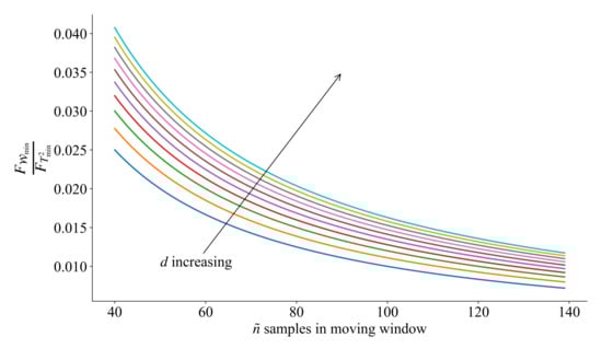
Figure 1. Sensitivity analysis.

4. Wasserstein Distance for Monitoring Non-Gaussian Process

Section 2 and Section 3 discussed how Wasserstein distance can be used to monitor Gaussian distributed process variables. However, in many industrial processes, process variables are often non-Gaussian distributed, whose PDFs can be difficult to estimate from data. In order to estimate the Wasserstein distance from non-Gaussian distributed data, this Section introduces the Riemannian block coordinate descent(RBCD) method for estimating Wasserstein distance between PDFs of non-Gaussian variables [29,37].

4.1. Riemannian Block Coordinate Descent for Estimation of Wasserstein Distance

This section considers the process monitoring problem under the multivariate statistical analysis framework, as projecting the original data space onto a low-dimensional subspace can effectively alleviate the curse of dimensionality. Let $\mathbf{z}$ and $\tilde{\mathbf{z}}$ be the d-dimensional score vectors obtained from non-Gaussian distributed data sources according to Equations (1) and (2). Instead of continuous probability measures, estimation of Wasserstein distance under the non-Gaussian case requires definition of discrete probability measures for $\mathbf{z}$ and $\tilde{\mathbf{z}}$ as $\mathbf{\mu }={\sum }_{i=1}^m{r}_i{\delta }_{{\mathbf{z}}_i}$ and $\mathbf{\nu }={\sum }_{k=1}^n{\tilde{r}}_k{\delta }_{{\tilde{\mathbf{z}}}_k}$, with $\mathbf{r}={(r_1,r_2,\cdots ,r_m)}^T$ and $\tilde{\mathbf{r}}={({\tilde{r}}_1,{\tilde{r}}_2,\cdots ,{\tilde{r}}_n)}^T$ being the probability simplex and $\delta$ the Dirac function. According to Ref. [29], computing the Wasserstein distance between $\mathbf{\mu }$ and $\mathbf{\nu }$ is equivalent to solving an optimal transport problem as follows.

$$\underset{\mathbf{R}\in \mathcal{M}}{max}\underset{\mathbf{\pi }\in \mathsf{\Pi }(\mathbf{\mu },\mathbf{\nu })}{min}\sum _{i=1}^m\sum _{k=1}^n{\mathbf{\pi }}_{ik}{∥{\mathbf{R}}^T{\mathbf{z}}_i-{\mathbf{R}}^T{\tilde{\mathbf{z}}}_k∥}^2$$

(32)

Here $\mathbf{R}\in {\mathbb{R}}^{d\times d^{\prime }}\left(1\le d^{\prime }<d\right)$ is the projection matrix defined in a Stiefel manifold $\mathcal{M}=\left\{\mathbf{R}\right.$$\in {\mathbb{R}}^{d\times d^{\prime }}|{\mathbf{R}}^T\mathbf{R}={\mathbf{I}}_{d^{\prime }\times d^{\prime }}\}$, $\mathsf{\Pi }(\mathbf{\mu },\mathbf{\nu })$ is the transportation polytope $\mathsf{\Pi }(\mathbf{\mu },\mathbf{\nu }):=\left\{\mathbf{\pi }\in {\mathbb{R}}^{m\times n}|\mathbf{\pi }\mathbf{1}=\mathbf{r},\right.$$\left.{\mathbf{\pi }}^T\mathbf{1}=\tilde{\mathbf{r}}\right\}$, $\mathbf{1}$ is the vector of ones. The purpose of introducing the projection matrix $\mathbf{R}$ is to reduce the computation load and increase robustness. As can be seen from Equation (32), the optimization problem is nonconvex and difficult to solve. In order to improve the computation efficiency, Lin et al. [37] considered the following entropy-regularized optimization problem.

$$\begin{array}{cc}\hfill & \underset{\mathbf{R}\in \mathcal{M}}{max}\underset{\mathbf{\pi }\in \mathsf{\Pi }(\mathbf{\mu },\mathbf{\nu })}{min}\sum _{i=1}^m\sum _{k=1}^n{\mathbf{\pi }}_{ik}{∥{\mathbf{R}}^T{\mathbf{z}}_i-{\mathbf{R}}^T{\tilde{\mathbf{z}}}_k∥}^2-\epsilon H\left(\mathbf{\pi }\right)\hfill \\ \hfill & s.t.\phi \left(\mathbf{\pi }\right)=\mathbf{\pi }\mathbf{1}=\mathbf{r},\rho \left(\mathbf{\pi }\right)={\mathbf{\pi }}^T\mathbf{1}=\tilde{\mathbf{r}},\mathbf{R}\in \mathcal{M}\hfill \end{array}$$

(33)

Here $H\left(\mathbf{\pi }\right)=-{\displaystyle \sum _{i,k}^{}}\left({\mathbf{\pi }}_{ik}log{\mathbf{\pi }}_{ik}-{\mathbf{\pi }}_{ik}\right)$ is the entropy regularization term and $\epsilon \ge 0$ is the regularization parameter. By introducing the entropy-regularization, Equation (33) can be effectively solved using the Riemannian block coordinate descent(RBCD) method [29] by alternatively estimating $\mathbf{R}$ and $\mathbf{\pi }$.

Assume $\mathbf{R}$ is determined, Equation (33) reduces to a convex problem with respect to $\mathbf{\pi }$ as follows.

$$\underset{{\mathbf{\beta }}_1,{\mathbf{\beta }}_2}{max}\underset{\mathbf{\pi }}{min}\sum _{i,k}^{}{\mathbf{\pi }}_{ik}{∥{\mathbf{R}}^T{\mathbf{z}}_i-{\mathbf{R}}^T{\tilde{\mathbf{z}}}_k∥}^2-\epsilon H\left(\mathbf{\pi }\right)+{\mathbf{\beta }}_1^T\left(\phi \left(\mathbf{\pi }\right)-\mathbf{r}\right)+{\mathbf{\beta }}_2^T\left(\rho \left(\mathbf{\pi }\right)-\tilde{\mathbf{r}}\right)$$

(34)

Here ${\mathbf{\beta }}_1$ and ${\mathbf{\beta }}_2$ are the Lagrange multipliers of the two equality constraints. Taking the first-order partial derivative of $\mathbf{\pi }$ and setting it to zero, it is easy to obtain $\mathbf{\pi }$ as follows.

$${\mathbf{\pi }}_{ik}=exp\left(\left(-{\mathbf{\beta }}_{1,i}-{\mathbf{\beta }}_{2,k}-{∥{\mathbf{R}}^T{\mathbf{z}}_i-{\mathbf{R}}^T{\tilde{\mathbf{z}}}_k∥}^2\right)/\epsilon \right)$$

(35)

with ${\mathbf{\beta }}_{1,i}$ being the i-th element of ${\mathbf{\beta }}_1$ and ${\mathbf{\beta }}_{2,k}$ is the k-th element of ${\mathbf{\beta }}_2$. The optimization problem in Equation (35) can be easily solved. It should be noted that once $\mathbf{\pi }$ is determined, the two discrete probability vectors $\mathbf{r}$ and $\tilde{\mathbf{r}}$ can be obtained.

By defining $\mathbf{u}=-{\mathbf{\beta }}_1/\epsilon$ and $\mathbf{v}=-{\mathbf{\beta }}_2/\epsilon$, Equation (35) is rewritten as follows.

$${\left[\mathbf{\pi }(\mathbf{u},\mathbf{v},\mathbf{R})\right]}_{ik}=exp\left(-\frac{1}{\epsilon }{∥{\mathbf{R}}^T({\mathbf{z}}_i-{\tilde{\mathbf{z}}}_k)∥}^2+{\mathbf{u}}_i+{\mathbf{v}}_k\right)$$

(36)

Noting that the optimality condition of the minimization problem in Equation (34) is Equation (36).

On the other hand, substituting Equation (36) into Equation (33), if $\mathbf{\pi }$ is determined, the optimization problem for $\mathbf{R}$, $\mathbf{u}$ and $\mathbf{v}$ can be defined as follows.

$$\underset{\mathbf{R}\in \mathcal{M},\mathbf{u},\mathbf{v}}{min}{\mathcal{W}}^{*}(\mathbf{u},\mathbf{v},\mathbf{R})=\sum _{i,k}^{}{\left[\mathbf{\pi }\left(\mathbf{u},\mathbf{v},\mathbf{R}\right)\right]}_{ik}-{\mathbf{r}}^T\mathbf{u}-{\tilde{\mathbf{r}}}^T\mathbf{v}$$

(37)

Solution of Equation (37) can be achieved using the RBCD iteration, which performs by updating one parameter each time while fixing other parameters. The detailed Riemannian optimization routines can be referred to Huang et al. [29].

The procedures of alternatively estimating $\mathbf{R}$ and $\mathbf{\pi }$ are conducted until convergence. On convergence, the estimation of Wasserstein distance under non-Gaussian data source can be defined as

$${\mathcal{W}}^{*}=min\sum _{i=1}^m\sum _{k=1}^n{\mathbf{\pi }}_{ik}{∥{\mathbf{R}}^T{\mathbf{z}}_i-{\mathbf{R}}^T{\tilde{\mathbf{z}}}_k∥}^2-\epsilon H\left(\mathbf{\pi }\right)$$

(38)

4.2. Process Statistics and Null Hypothesis Rejection Region

From the above discussion, the Wasserstein distance of non-Gaussian data can be estimated by RBCD method. Thus, it is necessary to establish corresponding monitoring statistic for fault detection. Since we calculate ${\mathcal{W}}^{*}$ from Section 4.1, statistic based on Wasserstein distance for non-Gaussian distributed data is given by:

$${\mathbb{W}}_k\left(\widehat{f},{\widehat{\tilde{f}}}^k\right)={\mathcal{W}}^{*}$$

(39)

where, k is the sample index. The control limit of the statistic can be estimated by kernel density estimation [38] with the significant level of $\alpha$. By replacing the ${\mathbb{W}}_k\left(\widehat{f},{\widehat{\tilde{f}}}^k\right)$ with ${\mathcal{W}}^{*}$ and replacing the control limit value ${\chi }_{1,\alpha }^2$ with the estimated PDF of ${\mathbb{W}}_k\left(\widehat{f},{\widehat{\tilde{f}}}^k\right)$ under normal condition, the online strategy introduced in Section 3.1 can be used to monitor non-Gaussian processes.

5. Fault Isolation Method Based on the Wasserstein Distance

Once a fault is detected, it becomes extremely important to isolate and identify faulty variables in time to facilitate subsequent correcting operations. Although researchers have made considerable progress in detection of incipient faults, fault isolation remains a problem for non-Gaussian distributed data. This section develops a fault isolation method based on the Wasserstein distance, so that a unified process monitoring framework for incipient faults can be constructed. Consider the fault model introduced in Equation (25), the optimization problem for fault isolation can be defined as follows.

$$\Delta \widehat{\mathbf{x}}=\underset{\Delta \mathbf{x}}{argmin}\sum _{i=1}^m\sum _{k=1}^{\tilde{n}}{\mathbf{\pi }}_{ik}\left(\left|\right|{\mathbf{R}}^T{\mathbf{w}}^T{\mathbf{x}}_i-{\mathbf{R}}^T{\mathbf{w}}^T\left({\overline{\mathbf{x}}}_k+\Delta \mathbf{x}\right){\left|\right|}^2+{\lambda \left|\right|\Delta \mathbf{x}\left|\right|}_1\right)$$

(40)

Here, $\Delta \widehat{\mathbf{x}}$ is the estimation of the true fault vector, $\lambda$ is the regularization parameter. It should be noted that by introducing the $l_1$ regularization term a sparse faulty variable set can be obtained [39]. The optimization problem in Equation (40) can be divided into a series of sub-problems.

$$\Delta {\widehat{\mathbf{x}}}_{ik}=\underset{\Delta {\mathbf{x}}_{ik}}{argmin}\left|\right|{\mathbf{R}}^T{\mathbf{w}}^T{\mathbf{x}}_i-{\mathbf{R}}^T{\mathbf{w}}^T\left({\overline{\mathbf{x}}}_k+\Delta {\mathbf{x}}_{ik}\right){\left|\right|}^2+\lambda \left|\right|\Delta {\mathbf{x}}_{ik}{\left|\right|}_1$$

(41)

As discussed in Section 4.1, after estimating the Wasserstein distance in a sub-window, $\mathbf{R}$ and $\mathbf{\pi }$ are fixed. Therefore, by denoting ${\mathbf{R}}^T{\mathbf{w}}^T\left({\mathbf{x}}_i-{\overline{\mathbf{x}}}_k\right)$ as dependent variables, ${\mathbf{R}}^T{\mathbf{w}}^T$ as independent variable and $\Delta {\widehat{\mathbf{x}}}_{ik}$ as regression coefficients, Equation (41) can be solved as Lasso regression problem. And the reconstructed fault vector can be described as:

$$\Delta \widehat{\mathbf{x}}=\frac{1}{m\tilde{n}}\sum _{i=1}^m\sum _{k=1}^{\tilde{n}}{\mathbf{\pi }}_{ik}\Delta {\widehat{\mathbf{x}}}_{ik}$$

(42)

Consequently, $\Delta {\widehat{\mathbf{x}}}_l$ obtained by Equation (42) is zero if the lth variable is normal, otherwise it is faulty. It is worth noting that $\mathbf{\pi }$ keeps changing as the sliding window moves and the estimation of $\Delta \mathbf{x}$ is related to $\mathbf{\pi }$ according to Equation (42), making the results more reliable and robust for dynamically changing data.

6. Application Studies

This section tests the effectiveness of the Wasserstein distance-based process monitoring method using application studies to a simulation example and a real-time boiler water wall over-temperature process.

6.1. Simulation Example

Consider a simulation example generated by the following multivariate process:

$$\mathbf{x}=\mathbf{Bs}+\mathbf{e}$$

(43)

Here, $\mathbf{B}=\left[\begin{array}{cccc}0.55& 0.72& 0.60& 0.54\\ 0.42& 0.65& 0.44& 0.89\\ 0.96& 0.38& 0.79& 0.53\\ 0.57& 0.93& 0.07& 0.09\\ 0.02& 0.83& 0.78& 0.87\\ 0.98& 0.80& 0.46& 0.78\end{array}\right]$. This simulation example involving six input variables defined as $\mathbf{x}={\left[x_1,\cdots ,x_6\right]}^T$, which are linear combination of four multivariate normal distribution data sources $\mathbf{s}={\left[s_1,\cdots ,s_4\right]}^T\sim \mathcal{N}\left(\mathbf{\mu },\mathbf{I}\right),\mathbf{\mu }={\left[1.2,0.7,2.3,1.7\right]}^T$, corrupted by Gaussian distributed noises $\mathbf{e}={\left[{\mathbf{e}}_1,\cdots ,{\mathbf{e}}_6\right]}^T\sim \mathcal{N}\left(\mathbf{0},{\mathsf{\Sigma }}_{\mathbf{e}}\right)$, ${\mathsf{\Sigma }}_{\mathbf{e}}=\mathrm{diag}\{0.031,0.023,0.192,$$0.173,0.150,0.113\}$.

For the purpose of model training, a total of 700 samples are generated as the training set. An additional 300 samples are generated as the test set, which involves a ramp fault on ${\mathbf{x}}_4$ as ${\widehat{\mathbf{x}}}_4={\mathbf{x}}_4+0.01\times (k-700),k=701,\cdots ,1000$. For the purpose of process monitoring, PCA is first applied and the Wasserstein distance based monitoring statistics are computed based on Equation (22) for the PCs and residuals. Based on the moving window approach proposed in Section 3.1, a series of monitoring statistics can be calculated. For the proposed method, a window length of 100 is considered and it is found that retaining 3 principal components (PCs) captures more than 95% variance, so that the number of PCs is set as 3. For comparison, PCA based method and an incipient fault detection method based on statistics Mahalanobis distance(SMD) [21] are considered. The window lengths for SMD is also set as 100. In addition, the significance level for all the three methods is set as 0.01 and the monitoring results are shown in Figure 2.

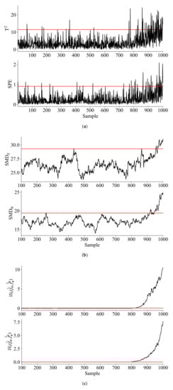
Figure 2. Monitoring results for the simulation example: (a) PCA (b) SMD (c) Wasserstein distance.

As is observed from Figure 2, the monitoring statistics of conventional PCA and SMD failed to detect the ramp fault in the early stage. In contrast, it can be seen that the ramp fault was successfully detected in both the principle component space and the residual space by the monitoring statistics based on Wasserstein distance. This is expected, as the sensitivity analysis in Section 3.2 shows that the monitoring statistics based on Wasserstein distance show higher sensitivity, indicating that it is suitable for monitoring of incipient faults. In order to further evaluate the performance of the proposed method, Table 1 presents the fault detection rate(FDR) and fault alarm rate(FAR) of the considered methods. Also, to indicate the performance for incipient fault detection, the time of first detection(TFD) is also presented.

Table 1. Comparison of fault detection performance for the simulation example.

	PCA		SMD		Wasserstein Distance
	T${}^2$	SPE	SMD${}_{\mathbf{z}}$	SMD${}_{\mathbf{e}}$	${\mathbb{W}}_{\mathit{k}}\left({\widehat{\mathit{f}}}_{\mathbf{z}},{\widehat{\tilde{\mathit{f}}}}_{\mathbf{z}}^{\mathit{k}}\right)$	${\mathbb{W}}_{\mathit{k}}\left({\widehat{\mathit{f}}}_{\mathbf{e}},{\widehat{\tilde{\mathit{f}}}}_{\mathbf{e}}^{\mathit{k}}\right)$
TFD	766	730	863	916	813	783
FDR	1.57%	1.20%	13.67%	23.33%	62.00%	70.67%
FAR	0.7%	0.9%	0.17%	0.17%	0.17%	0.17%

Table 1 confirms that the monitoring statistics based on Wasserstein distance outperform those of PCA and SMD. More specifically, the ${\mathbb{W}}_k\left({\widehat{f}}_{\mathbf{e}},{\widehat{\tilde{f}}}_{\mathbf{e}}^k\right)$ statistic for Wasserstein distance has an FDR of 70.67%. In contrast, the FDRs for PCA based statistics are lower than 5% and those for SMD are lower than 30%.

6.2. Application to a CSTR Process

This section discusses the effectiveness of the proposed method in a CSTR process [40]. The dynamic characteristics of the CSTR process can be described by material conservation and energy conservation respectively,

$$\begin{array}{c}\frac{dC}{dt}=\frac{F}{V}\left(C_0-C\right)-k_0{e}^{-\frac{E}{RT}}C+v_1\end{array}$$

(44a)

$$\begin{array}{c}\frac{dT}{dt}=\frac{F}{V}\left(T_0-T\right)+\frac{-\Delta H}{\rho C_p}{k}_0{e}^{-\frac{E}{RT}}C+\frac{UA}{V\rho C_p}\left(T_C-T\right)+v_2\end{array}$$

(44b)

where $C_0$ is the reactor inlet concentration, C is the outlet concentration, F is the flow rate at the reactor inlet, T is the reaction temperature, $T_0$ is the reactor inlet temperature, $T_C$ is the cooling water temperature and $v_1$, $v_2$ are independent noise, other variables are described in Table 2, the parameters and conditions of the whole process are the same as in Li et al. [41] and Ji et al. [42].

Table 2. CSTR process variable description and its initial value.

Variable	Description	Initial Value
$-\Delta H$	Chemical reaction heat	17,835.821 J/mol
$\rho$	Solvent density	1000 g/L
$E/R$	Activation energy and gas constant	5360 K
V	Reactor volume	100 L
$UA$	Thermal Conductivity	11,950 J/(min K)
$k_0$	Arrhenius reaction rate constant	exp(13.4) min${}^{-1}$
$C_p$	Reactant specific heat	0.239 J/(gK)
$C_0$	Reactor inlet concentration	1 mol/L
T	Reaction temperature	446 K
$T_C$	Cooling water temperature	419 K
F	Flow rate at the reactor inlet	100 L/min
$T_0$	Reactor inlet temperature	400 K
$v_1,v_2$	Gaussian noise	$\mathcal{N}(0,0.01)$

In order to describe the dynamic and non-linearity of this process, we define ${\tau }_1=\frac{C_0-C}{C_0}$, ${\tau }_2=\frac{\gamma \left(T-T_0^{*}\right)}{T_0^{*}}$, $u=\frac{\gamma \left(T_C-T_0^{*}\right)}{T_0^{*}}$ and $\xi =\frac{\gamma \left(T_0-T_0^{*}\right)}{T_0^{*}}$, then Equations (44a) and (44b) are normalized using dimensionless variable ${\zeta }_1$, ${\zeta }_2$, u and $\xi$ [43,44],

$$\begin{array}{c}{\dot{\tau }}_1=-{\theta }_1{\tau }_1+D_{{\theta }_1}(1-{\tau }_1)e^{\frac{{\tau }_2}{1+{\tau }_2/\gamma }}\end{array}$$

(45a)

$$\begin{array}{c}{\dot{\tau }}_2=-{\theta }_1{\tau }_2+B{D}_{{\theta }_1}(1-{\tau }_1)e^{\frac{{\tau }_2}{1+{\tau }_2/\gamma }}-{\theta }_2{\tau }_2+{\theta }_{2}u+{\theta }_1\xi \end{array}$$

(45b)

where, $\gamma =\frac{E}{RT}$, $B=\frac{\gamma \Delta HC}{C_p{T}_0^{*}}$, $D_{{\theta }_1}=k_0{e}^{(-\gamma )}$, ${\theta }_1=\frac{V}{F}$ and ${\theta }_2=\frac{UA}{V\rho C_p}$, $\dot{{\tau }_1}$ ($\dot{{\tau }_2}$) represents the first derivative with respect to ${\tau }_1$ (${\tau }_2$). Thus, Equations (45)a,b can be regarded as a nonlinear mathematical model. Since we study the ideal CSTR process, it contains the following assumptions [45], (1) composition and temperature are uniform everywhere in the tank; (2) the effluent composition is the same as that in the tank; and (3) the tank operates at steady state.

The sample measured in this system contains six variables, i.e., $\mathbf{x}={[C,T,T_C,F,C_0,T_0]}^T$. Here, C and T are the controlled objects with nomianl values, $T_C$ and F are the controllable variables with feedback from control errors and the negative feedback inputs are added to $T_C$ and F through the transfer function form of the PID controller (P = 1, I = 10, D = 0.1), $C_0$ and $T_0$ are the input variables. The sampling interval of the system is 1 second and 1000 sampling points under normal conditions are collected as training data. In order to verify the validity of the algorithm, a fault is artificially assumed, a sensor bias fault of 5 L/min is applied to the fourth variable F at 1001∼1600 samples, which can be seen as an incipient fault since this bias is small for the initial value.

It is worth noting that the collected data is non-Gaussian distributed and noisy, the proposed method introduced in Section 4 is used, with the learning rate and penalty parameter set as 0.1 and 0.5, also compared with PCA and SMD. It is found that retaining 4 principal components (PCs) is able to capture more than 80% variance, hence the number of PCs is set as 4. The window lengths used for SMD method and the proposed method are both 100. The significance level is set as 0.01 for all the methods and the monitoring results are shown in Figure 3.

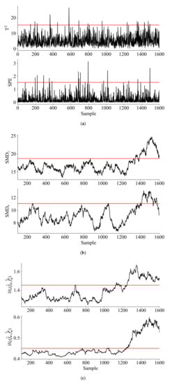
Figure 3. Monitoring results for the CSTR process: (a) PCA (b) SMD (c) Wasserstein distance.

It can be seen from Figure 3 that the proposed method can detected fault at the early stage, while PCA and SMD failed to detect the fault. Table 3 shows the detailed results of TFD, FDR and FAR for the three methods.

Table 3. Comparison of fault detection performance on CSTR.

	PCA		SMD		Wasserstein Distance
	T${}^2$	SPE	SMD${}_{\mathbf{z}}$	SMD${}_{\mathbf{e}}$	${\mathbb{W}}_{\mathit{k}}\left({\widehat{\mathit{f}}}_{\mathbf{z}},{\widehat{\tilde{\mathit{f}}}}_{\mathbf{z}}^{\mathit{k}}\right)$	${\mathbb{W}}_{\mathit{k}}\left({\widehat{\mathit{f}}}_{\mathbf{e}},{\widehat{\tilde{\mathit{f}}}}_{\mathbf{e}}^{\mathit{k}}\right)$
TFD	1237	1196	1346	1400	1123	1027
FDR	1.60%	1.00%	40.16%	26.83%	65.50%	62.00%
FAR	1.40%	1.10%	0.11%	0.33%	0.62%	0.11%

Table 3 confirmed that the monitoring statistics based on Wasserstein distance have better performance for both FDR and FAR. Specifically, the monitoring statistics ${\mathbb{W}}_k\left({\widehat{f}}_{\mathbf{e}},{\widehat{\tilde{f}}}_{\mathbf{e}}^k\right)$ of Wasserstein distance identified the bias fault at sample No.1027, significantly earlier than the method of SMD.

In order to isolate the bias fault, the method proposed in Section 5 is applied and the regularization parameter $\lambda$ is set as 0.001. Also, we compare the proposed method with the BRNN with LDR-based fault isolation method [27]. Figure 4 presents the sample-by-sample fault isolation result, the darker the color in the figure, the greater the fault score of this sampling point and the fault contribution during the process.

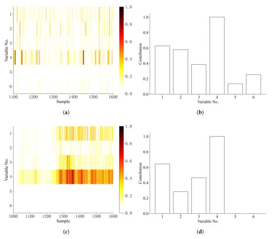
Figure 4. Fault isolation results for the CSTR process (a) BRNN with LDR isolation (b) BRNN with LDR contribution (c) Wasserstein distance isolation (d) Wasserstein distance contribution.

From Figure 4 is can be seen that the fourth variable was successfully identified as faulty using the Wasserstein distance based fault isolation method, this is in accordance with the previous setting. Though BRNN can identify $x_4$ as the fault variable, it cannot obtain sparse fault isolation results and is not sensitive to the fault.

6.3. Application to a Boiler Water Wall Over-Temperature Process

This section discusses the effectiveness of the proposed method on a real-time boiler water wall data. The water wall is an important part of the boiler system, which is a neatly arranged metal pipe that clings to the inside of the furnace. Its function is to absorb the radiant heat of the high temperature flame or flue gas in the furnace, generate steam or hot water in the tube, and reduce the temperature of the furnace wall to protect the furnace wall. Due to its material properties, the water wall has a corresponding limit to withstand temperature. In this example, the limit temperature is 460 ℃, which is provided by the boiler producer according to their design specifications. Working above the limit temperature for long will lead to the severe accident of burnout of tubes. So, it is also important to keep the absolute temperature of water wall tubes below the limit temperature to ensure safety. In order to minimize the losses caused by the overtemperature of the water wall, it is necessary to monitor the variables that affect the temperature of the water wall. The temperature of the water wall in this case rises slowly, which can be considered as an incipient fault in the industrial process.

Figure 5 shows the process flow chart of coal-fired power plant. It can be seen from the figure that after the coal enters the coal box, it is sent to the coal mill to be ground into pulverized coal and the air is preheated after entering the blower, and then divided into primary air and secondary air, the primary air contains air and pulverized coal. The primary air and secondary air enter the boiler for combustion after passing through the baffle, and the boiler feed water is heated to generate superheated steam to drive the generator to generate electricity. After combustion, coal ash and waste gas are removed from the system.

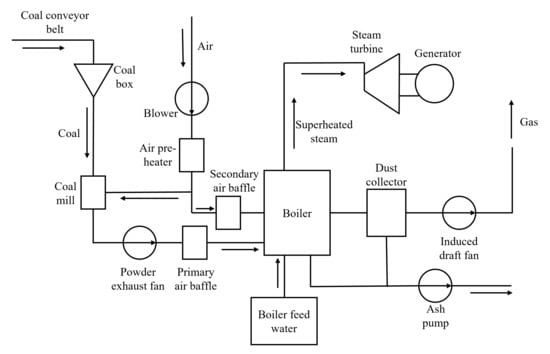
Figure 5. Process flow chart of coal-fired power plant.

In this process, a total of 10 variables are considered and listed in Table 4. Samples are collected every 15 seconds for each variable, and a total 1100 sample points are collected, including 600 normal samples and 500 faulty samples. The fault occurs when the positional deviation of the secondary air baffle causes the deviant combustion of the flame, and the primary wind speed deviation causes the flame to brush the wall. In addition, the sample data is non-Gaussian, and there is no obvious correlation between variables in a long sampling period.

Table 4. Variables and description for boiler water wall over-temperature process.

Variable	Description
$x_1$	Boiler feed water valve inlet pressure
$x_2$	Boiler feed water temperature
$x_3$	Boiler load
$x_4$	Water to coal ratio
$x_5$	Total air flow
$x_6$	Furnace pressure
$x_7$	Primary air baffle position
$x_8$	Secondary air baffle position
$x_9$	Feedback signal of coal feeding amount of coal feeder
$x_{10}$	primary airflow speed

Similar to Section 6.1, PCA is first applied and the Wasserstein distance based monitoring statistics are computed using the RBCD algorithm in Section 4, with the learning rate and penalty parameter set as 0.1 and 1.6. It is found that retaining 4 principal components (PCs) captures more than 85% variance so that the number of PCs is set as 4. The window lengths used for SMD method and the proposed method are both 100. The significance level is equally set as 0.01 for all the methods and the monitoring results are shown in Figure 6.

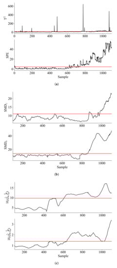
Figure 6. Monitoring results for the boiler water wall over-temperature process: (a) PCA (b) SMD (c) Wasserstein distance.

Figure 6 shows that the fault is successfully detected by all the three methods at the later stage. However, at the early stage, PCA and SMD failed to detect the fault, indicating they are not sensitive enough for this fault. In contrast, the monitoring statistics based on Wasserstein distance successfully detected the fault at an earlier stage. Table 3 shows the comparison results of TFD, FDR and FAR for the three methods.

From Table 5 it can be seen that the monitoring statistics based on Wasserstein distance shows much higher FDR than other methods. A closer inspection also shows that the monitoring statistic ${\mathbb{W}}_k\left({\widehat{f}}_{\mathbf{z}},{\widehat{\tilde{f}}}_{\mathbf{z}}^k\right)$ of Wasserstein distance identified the fault at the earliest stage at sample No.607, which further verified the previous results on sensitivity analysis.

Table 5. Comparison of fault detection performance on boiler water wall over-temperature process.

	PCA		SMD		Wasserstein Distance
	T${}^2$	SPE	SMD${}_{\mathbf{z}}$	SMD${}_{\mathbf{e}}$	${\mathbb{W}}_{\mathit{k}}\left({\widehat{\mathit{f}}}_{\mathbf{z}},{\widehat{\tilde{\mathit{f}}}}_{\mathbf{z}}^{\mathit{k}}\right)$	${\mathbb{W}}_{\mathit{k}}\left({\widehat{\mathit{f}}}_{\mathbf{e}},{\widehat{\tilde{\mathit{f}}}}_{\mathbf{e}}^{\mathit{k}}\right)$
TFD	625	621	870	857	607	634
FDR	39.60%	81.80%	31.20%	48.80%	98.6%	92.4%
FAR	1.33%	0.83%	1.00%	0.25%	0.40%	0.80%

As for fault isolation, the regularization parameter $\lambda$ is set as 0.02 in our method. Also, we compare the proposed method with the BRNN with LDR-based fault isolation method [27]. Figure 6 and gives the sample-by-sample fault isolation results and the fault contribution during the process.

It can be seen from Figure 7 that Wasserstein distance based method can isolate faulty variable $x_8$ and $x_{10}$ at an early stage and The fault contribution values of $x_8$ and $x_{10}$ are the largest. This indicates that the failure of the position of the secondary air baffle position and the primary wind speed caused the overtemperature of the water wall, which is consistent with the actual situation. While BRNN with LDR-based method can isolate $x_8$ successfully, the fault scores of $x_{10}$ is not that significant comparing to other variables.

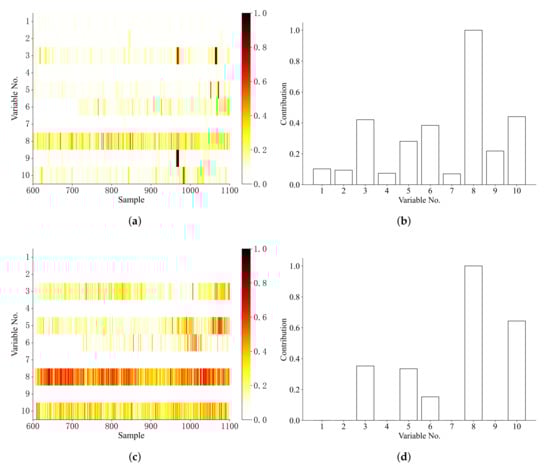
Figure 7. Fault isolation results for the boiler over-temperature process (a) BRNN with LDR isolation (b) BRNN with LDR contribution (c) Wasserstein distance isolation (d) Wasserstein distance contribution.

7. Conclusions

This paper proposes an incipient fault detection method based on Wasserstein distance of industrial systems. For both Gaussian and non-Gaussian cases, a theoretical model is proposed and widely show the effectiveness of Wasserstein distance for fault detection. It is found that there is a normally distributed relationship between the empirical estimated value and the true value of Wasserstein distance, a confidence limit based on Wasserstein distance of two Gaussian data sets can be easily obtained. The sensitivity of Wasserstein distance is compared with Hotelling’s $T^2$ statistics, which increases as the number of variable increases. For the source signals do not have a Gaussian distribution, we proposed a RBCD method under the PCA framework. We use PCA to project high-dimensional data into low-dimensional space to establish a projection robust Wasserstein distance model, a Riemannian block coordinate descent algorithm is adopted to speed up the solution of the model and the monitoring method is then test on fault monitoring of a simulation example, a CSTR process and a real-time boiler water wall over-temperature process. After detecting the fault, we proposed a reconstruction method based on Wasserstein distance to isolate fault. The fault detection based on Wasserstein distance is then compared with other fault detection methods and the results show that it has better sensitivity and higher fault detection rate. Future work on the Wasserstein distance-based fault detection method could be extended to nonlinear and time-varying industrial processes.

References

- Liu, Y.; Zeng, J.; Bao, J.; Xie, L. A unified probabilistic monitoring framework for multimode processes based on probabilistic linear discriminant analysis. IEEE Trans. Ind. Inform. 2020, 16, 6291–6300. [Google Scholar] [CrossRef]
- Ge, Z. Review on data-driven modeling and monitoring for plant-wide industrial processes. Chemom. Intell. Lab. Syst. 2017, 171, 16–25. [Google Scholar] [CrossRef]
- Jolliffe, I.T.; Cadima, J. Principal component analysis: A review and recent developments. Philos. Trans. R. Soc. A Math. Phys. Eng. Sci. 2016, 374, 20150202. [Google Scholar] [CrossRef] [PubMed]
- Ajami, A.; Daneshvar, M. Data driven approach for fault detection and diagnosis of turbine in thermal power plant using Independent Component Analysis (ICA). Int. J. Electr. Power Energy Syst. 2012, 43, 728–735. [Google Scholar] [CrossRef]
- Zhong, K.; Han, M.; Qiu, T.; Han, B. Fault diagnosis of complex processes using sparse kernel local fisher discriminant analysis. IEEE Trans. Neural Netw. Learn. Syst. 2020, 31, 1581–1591. [Google Scholar] [CrossRef] [PubMed]
- Yin, S.; Ding, S.X.; Xie, X.; Luo, H. A review on basic data-driven approaches for industrial process monitoring. IEEE Trans. Ind. Electron. 2014, 61, 6418–6428. [Google Scholar] [CrossRef]
- Zhu, J.; Ge, Z.; Song, Z.; Zhou, L.; Chen, G. Large-scale plant-wide process modeling and hierarchical monitoring: A distributed Bayesian network approach. J. Process Control 2018, 65, 91–106. [Google Scholar] [CrossRef]
- Zhao, Y.; He, X.; Zhang, J.; Ji, H.; Zhou, D.; Pecht, M.G. Detection of intermittent faults based on an optimally weighted moving average T2 control chart with stationary observations. Automatica 2021, 123, 109298. [Google Scholar] [CrossRef]
- Zeng, J.; Kruger, U.; Geluk, J.; Wang, X.; Xie, L. Detecting abnormal situations using the Kullback–Leibler divergence. Automatica 2014, 50, 2777–2786. [Google Scholar] [CrossRef]
- Qin, Y.; Yan, Y.; Ji, H.; Wang, Y. Recursive correlative statistical analysis method with sliding windows for incipient fault detection. IEEE Trans. Ind. Electron. 2021, 69, 4184–4194. [Google Scholar] [CrossRef]
- Zeng, J.; Xie, L.; Kruger, U.; Gao, C. Regression-based analysis of multivariate non-Gaussian datasets for diagnosing abnormal situations in chemical processes. AIChE J. 2014, 60, 148–159. [Google Scholar] [CrossRef]
- Shang, J.; Chen, M.; Ji, H.; Zhou, D. Recursive transformed component statistical analysis for incipient fault detection. Automatica 2017, 80, 313–327. [Google Scholar] [CrossRef]
- He, Z.; Shardt, Y.A.; Wang, D.; Hou, B.; Zhou, H.; Wang, J. An incipient fault detection approach via detrending and denoising. Control Eng. Pract. 2018, 74, 1–12. [Google Scholar] [CrossRef]
- Ji, H.; He, X.; Shang, J.; Zhou, D. Incipient fault detection with smoothing techniques in statistical process monitoring. Control Eng. Pract. 2017, 62, 11–21. [Google Scholar] [CrossRef]
- Zhao, C.; Huang, B. Incipient fault detection for complex industrial processes with stationary and nonstationary hybrid characteristics. Ind. Eng. Chem. Res. 2018, 57, 5045–5057. [Google Scholar] [CrossRef]
- Harmouche, J.; Delpha, C.; Diallo, D. Incipient fault detection and diagnosis based on Kullback–Leibler divergence using principal component analysis: Part I. Signal Process. 2014, 94, 278–287. [Google Scholar] [CrossRef]
- Chen, H.; Jiang, B.; Lu, N. An improved incipient fault detection method based on Kullback-Leibler divergence. ISA Trans. 2018, 79, 127–136. [Google Scholar] [CrossRef]
- Xiong, Y.; Chen, T. Abnormality detection based on the Kullback-Leibler divergence for generalized Gaussian data. Control Eng. Pract. 2019, 85, 257–270. [Google Scholar] [CrossRef]
- Cao, Y.; Jan, N.; Huang, B.; Fang, M.; Wang, Y.; Gui, W. Multimode process monitoring based on variational Bayesian PCA and Kullback-Leibler divergence between mixture models. Chemom. Intell. Lab. Syst. 2021, 210, 104230. [Google Scholar] [CrossRef]
- Zhang, X.; Delpha, C.; Diallo, D. Incipient fault detection and estimation based on Jensen–Shannon divergence in a data-driven approach. Signal Process. 2020, 169, 107410. [Google Scholar] [CrossRef]
- Ji, H. Statistics Mahalanobis distance for incipient sensor fault detection and diagnosis. Chem. Eng. Sci. 2021, 230, 116233. [Google Scholar] [CrossRef]
- Yang, J.; Delpha, C. An incipient fault diagnosis methodology using local Mahalanobis distance: Detection process based on empirical probability density estimation. Signal Process. 2022, 190, 108308. [Google Scholar] [CrossRef]
- Harmouche, J.; Delpha, C.; Diallo, D. Incipient fault amplitude estimation using KL divergence with a probabilistic approach. Signal Process. 2016, 120, 1–7. [Google Scholar] [CrossRef][Green Version]
- Ji, H.; He, X.; Zhou, D. Exponential smoothing reconstruction approach for incipient fault isolation. Ind. Eng. Chem. Res. 2018, 57, 6353–6363. [Google Scholar] [CrossRef]
- Yang, J.; Yang, Y.; Xie, G. Diagnosis of incipient fault based on sliding-scale resampling strategy and improved deep autoencoder. IEEE Sens. J. 2020, 20, 8336–8348. [Google Scholar] [CrossRef]
- Jana, D.; Patil, J.; Herkal, S.; Nagarajaiah, S.; Duenas-Osorio, L. Cnn and convolutional autoencoder (cae) based real-time sensor fault detection, localization, and correction. Mech. Syst. Signal Process. 2022, 169, 108723. [Google Scholar] [CrossRef]
- Sun, W.; Paiva, A.R.; Xu, P.; Sundaram, A.; Braatz, R.D. Fault detection and identification using bayesian recurrent neural networks. Comput. Chem. Eng. 2020, 141, 106991. [Google Scholar] [CrossRef]
- Arjovsky, M.; Chintala, S.; Bottou, L. Wasserstein GAN. arXiv 2017, arXiv:1701.07875. [Google Scholar]
- Huang, M.; Ma, S.; Lai, L. A riemannian block coordinate descent method for computing the projection robust wasserstein distance. In Proceedings of the International Conference on Machine Learning, PMLR, Virtual Event, 18–24 July 2021; pp. 4446–4455. [Google Scholar]
- Rüschenorf, L. Wasserstein Metric. In Encyclopedia of Mathematics; Hazewinkel, M., Ed.; Springer: Berlin/Heidelberg, Germany, 2001. [Google Scholar]
- Rudolf, D.; Schweizer, N. Perturbation theory for Markov chains via Wasserstein distance. Bernoulli 2018, 24, 2610–2639. [Google Scholar] [CrossRef]
- Villani, C. Optimal Transport: Old and New; Springer: Berlin/Heidelberg, Germany, 2009; Volume 338. [Google Scholar]
- Givens, C.R.; Shortt, R.M. A class of Wasserstein metrics for probability distributions. Mich. Math. J. 1984, 31, 231–240. [Google Scholar] [CrossRef]
- Rippl, T.; Munk, A.; Sturm, A. Limit laws of the empirical Wasserstein distance: Gaussian distributions. J. Multivar. Anal. 2016, 151, 90–109. [Google Scholar] [CrossRef]
- Ruymgaart, F.H.; Yang, S. Some applications of Watson’s perturbation approach to random matrices. J. Multivar. Anal. 1997, 60, 48–60. [Google Scholar] [CrossRef]
- Ver Hoef, J.M. Who invented the delta method? Am. Stat. 2012, 66, 124–127. [Google Scholar] [CrossRef]
- Lin, T.; Fan, C.; Ho, N.; Cuturi, M.; Jordan, M.I. Projection robust Wasserstein distance and Riemannian optimization. arXiv 2020, arXiv:2006.07458. [Google Scholar]
- Silverman, B.W. Density Estimation for Statistics and Data Analysis; Routledge: Oxfordshire, UK, 2018. [Google Scholar]
- Yan, Z.; Yao, Y. Variable selection method for fault isolation using least absolute shrinkage and selection operator (LASSO). Chemom. Intell. Lab. Syst. 2015, 146, 136–146. [Google Scholar] [CrossRef]
- Donghua, Z.; Yinzhong, Y. Modern Fault Diagnosis and Fault Tolerant Control; Tsing Hua University Publishing House: Beijing, China, 2000. [Google Scholar]
- Li, G.; Qin, S.J.; Ji, Y.; Zhou, D. Reconstruction based fault prognosis for continuous processes. Control Eng. Pract. 2010, 18, 1211–1219. [Google Scholar] [CrossRef]
- Ji, H.; He, X.; Shang, J.; Zhou, D. Incipient sensor fault diagnosis using moving window reconstruction-based contribution. Ind. Eng. Chem. Res. 2016, 55, 2746–2759. [Google Scholar] [CrossRef]
- Ghaffari, V.; Naghavi, S.V.; Safavi, A. Robust model predictive control of a class of uncertain nonlinear systems with application to typical cstr problems. J. Process Control 2013, 23, 493–499. [Google Scholar] [CrossRef]
- Wu, F. Lmi-based robust model predictive control and its application to an industrial cstr problem. J. Process Control 2001, 11, 649–659. [Google Scholar] [CrossRef]
- Foutch, G.L.; Johannes, A.H. Reactors in process engineering. In Encyclopedia of Physical Science and Technology, 3rd ed.; Meyers, R.A., Ed.; Academic Press: Cambridge, MA, USA, 2003; pp. 23–43. [Google Scholar]
Publisher’s Note: MDPI stays neutral with regard to jurisdictional claims in published maps and institutional affiliations. |
© 2022 by the authors. Licensee MDPI, Basel, Switzerland. This article is an open access article distributed under the terms and conditions of the Creative Commons Attribution (CC BY) license (https://creativecommons.org/licenses/by/4.0/).