Development of Artificial Neural Networks to Predict the Effect of Tractor Speed on Soil Compaction Using Penetrologger Test Results

Abstract

African agriculture is adversely impacted by arable soil compaction, the degree of which is affected by the speed at which the tractor is maneuvered on the fields, which affects the degree of soil compaction. However, there is no reliable, existing mathematical correlation between the extent of compaction on the one hand, and the tractor speed/s and soil moisture levels on the other. This paper bridges this gap in knowledge by resorting to the artificial neural networks (ANNs) method to predict the effects of tractor speed and soil moisture on the state of soil compaction. The models were ‘trained’ with penetration resistance (CPR) and bulk density test data obtained from field measurements. The resulting correlation coefficient (R = 0.9) showed good compliance of the prediction made with the ANN models with on-field data. It follows, thereby, that the model developed by the authors in this study can be effectively used for predicting the effects of speed, soil density, and moisture content on compaction of alluvial, poorly developed soil with much greater precision, thereby providing guidance to farmers around the world.

1. Introduction

Soil compaction is an aspect that is studied and researched by geotechnical engineers [1]. If we narrow down our focus to arable soil harnessed by the global agricultural sector, the imperative of feeding the growing population of the world—expected to reach 9 billion individuals by 2050—comes to mind [2]. It follows from this statistic that the cultivation of crops for supply to the food processing sector will have to increase by 70%. While this will necessitate the use of heavy machinery for harvesting, cropping, and other on-field farming activities, the risk of soil compaction will be greater, leading to soil degradation affecting an arable expanse of 68 million hectares [3,4]. Soil compaction can in turn be the cause of a host of adverse agronomic and environmental effects such as soil erosion, flooding, chemical leaching, surface water run-off, and emission of greenhouse gases [5,6,7]. The essential ecological functions of the soil are disrupted—porosity (the proportion of larger-sized pores), air-holding capacity, water infiltration capacity, and hydraulic conductivity decrease markedly [8,9,10]. In West Africa, reportedly, soil compaction has reduced crop yield by 40% to 90% [11,12]. It must, however, be noted here that it is not just the tractor-operation on the soil that is culpable, but also natural processes such as freezing, drying, swelling, and shrinking [13,14,15,16,17]. The soil has a certain degree of elasticity and thereby can resist externally applied stress to some extent, beyond which it becomes permanently (plastically) deformed [18,19].

Mechanically induced soil compaction, attributable to machinery and implements used by farmers, can be better understood by factoring in such operational variables as axle load, speed of the machine passages, number of passes, tire design, and inflation pressure [17,20,21,22,23,24,25]. Although the speed of machine passages contributes less, vis-à-vis the other variables, there is a direct correlation between the degree of soil compaction and the duration over which the external stress is applied. In other words, even though the dynamic effects—yawing, pitching, and accelerating—do increase the applied stress, a higher velocity tends to offset the effect to some extent [8,26].

In addition to these mechanical parameters related to the use of machinery on the soil, the moisture content of the arable soil is also a factor contributing to compaction [10,27,28,29]. Owing to the plethora of factors influencing the compaction, an accurate theoretical model has been difficult to construct. This has been overcome of late by taking recourse to artificial intelligence (AI) techniques such as artificial neural networks (ANNs) [30,31,32,33,34]. The use of ANN has enabled

• Determination of land cover [35].
• Modelling the dying kinetics of sesame seeds and proving that this technique was superior to traditional statistical modelling [36].
• Modelling soil properties in a better way than by using multivariate regression analysis [37].
• Predicting sugar diffusion capacity depending on the date-fruit variety, temperature, and spreading period.
• Predicting organic potato yield using tillage systems and soil properties as variables [5].

This study aims to

• Assess the impacts of tractor forward speed on the penetration resistance (PR) offered by the soil and the bulk density of the soil under different moisture level conditions.
• Evaluate the potential/capability of ANN to predict the degree of soil compaction from various sets of input data variables.

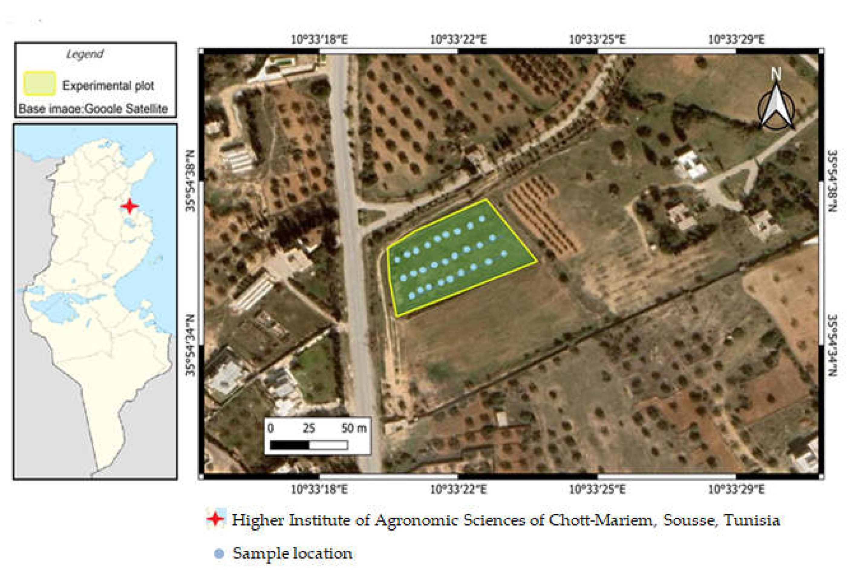
2. Materials and Methods

2.1. Experimental Site and Conditions

The experimental study was carried out on poorly developed alluvial soil at the Higher Institute of Agronomic Sciences of Chott-Mariem, Sousse University, Tunisia (depicted in Figure 1). The choice of location is guided by the fact that soil compaction is a common concern in the semi-arid/arid regions of Africa, and vast tracts of topsoil in North Africa conceal dense sub-soils beneath them. The location can be precisely described by the coordinates 35°54′40.2″ N 10°33′24.3″ E. The mean annual air temperature and annual precipitation at the location are 21 °C and 350 mm, respectively. The main soil characteristics of the 0–30 cm-layer horizon inserted can be listed as under:

• Sand particles (2000–50 μm), 480 g/kg of soil;
• Silt (50–2 μm), 300 g/kg of soil;
• Clay (less than 2 μm), 210 g/kg of soil.

Figure 1. Google Earth image and position of the Higher Institute of Agronomic Sciences of Chott-Mariem, Sousse, Tunisia. The yellow box indicates the boundary of the experimental plot, and the blue points indicate sample locations.

Figure 1. Google Earth image and position of the Higher Institute of Agronomic Sciences of Chott-Mariem, Sousse, Tunisia. The yellow box indicates the boundary of the experimental plot, and the blue points indicate sample locations.

The main crop cultivated on this alluvial soil is organic potato tilled conventionally with mold-board ploughing at a maximum depth of 30 cm. The soil organic matter content at the site was 1.2%. Soil organic matter at the experimental site was 1.2% at the time of the experiment. The experimental layout included tractor forward speed and soil moisture as the study factors. Two tractor forward speeds under three different soil moisture content scenarios were used in a completely randomized design (Figure 2). Each treatment was replicated 3 times: (C0: control, C1: speed₁ = 4 km/h, C2: speed₂ = 9 km/h), H0 (initial water content), H1 (water content after 15 days), and H2 (water content after 30 days). The tractor used for this experiment was the Foton TA700 with a total mass of 3.1 tonnes, power of 51 kW, and standard wheel-drive with a single rear-tire.

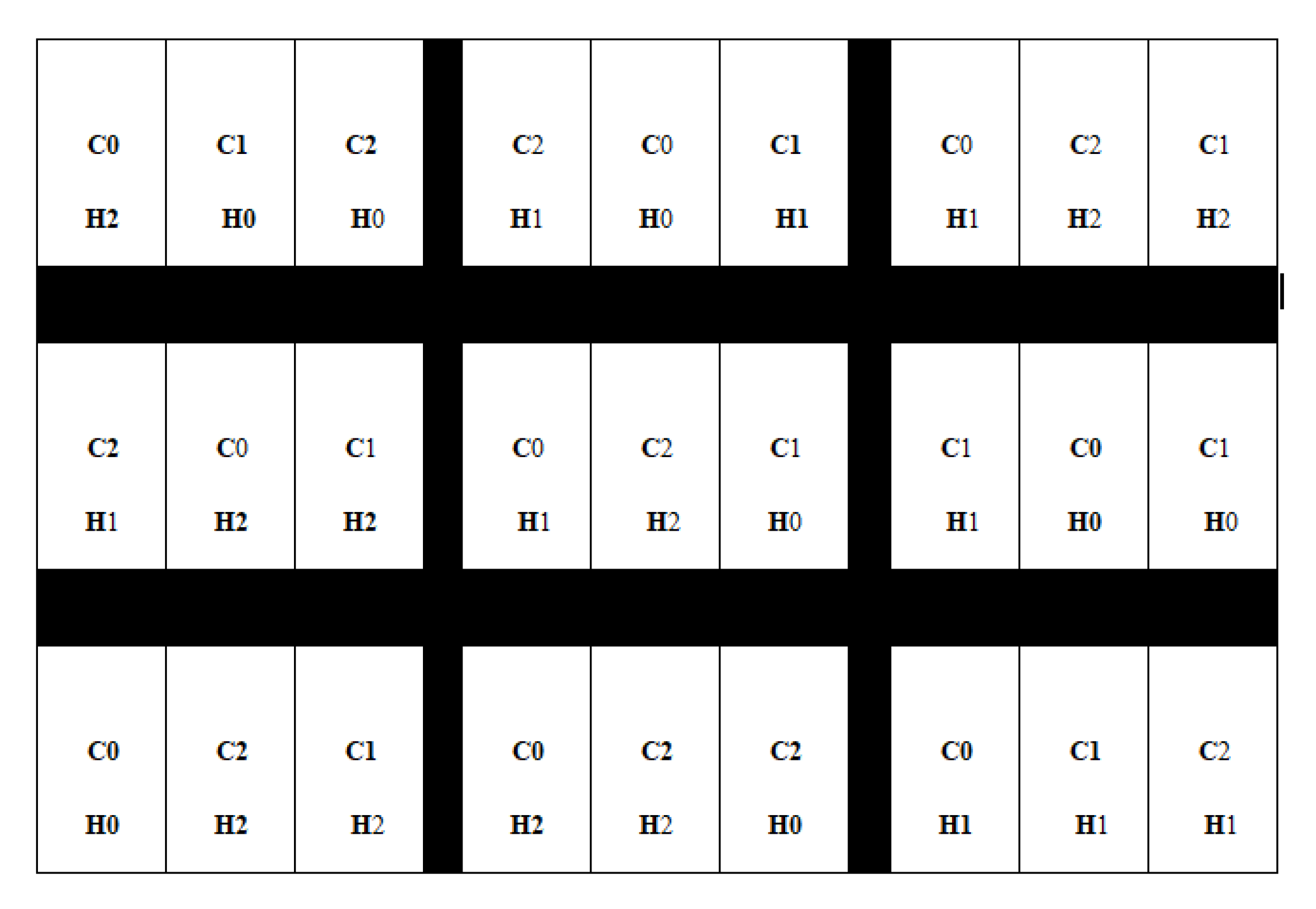
2.2. Soil Sampling and Analysis

Eighty-one undisturbed soil cores were randomly collected at depths of 10, 20, and 30 cm, using a portable soil sampler with steel cylinders (5 cm in height and diameter). Three similar samples were picked up from each layer. These were dried at 105 °C for 24 h in an oven. The bulk density (BD, Mg/m³) was determined by dividing the soil sample’s dry mass by the cylinder volume. The gravimetric water content, W (gkg⁻¹), was calculated as the mass of water in the soil sample divided by the mass of the dry soil. The organic matter content was calculated by wet oxidation [29]. The penetration resistance (CPR) is widely used to estimate the degree of compaction [38,39,40]. It is, simply put, the resistance of the soil to the force of penetration per unit area expressed in Nm⁻² or in MPa.

CPR was measured with a penetrologger (Eijkelkamp, Giesbeek, The Netherlands) to a depth of 50 cm. This device associates an electronic penetrometer to a built-in datalogger for storage and processing. It measures the mean vertical stress necessary for a cone penetration of 11.28 mm. The penetration depth is measured continuously as the cone is pressed within the soil. The operating range is 0–10 MPa (with a resolution of 0.01 MPa), and the measuring depth is from the surface down to 0.5 m (vertical resolution of 0.01 m) [5]. The penetration resistance is greatly affected by soil water content, soil texture, organic matter content, penetration speed, the length, and the cone tip angle [41]. The CPR was measured at about 108 measurement points; the penetration speed was 0.02 m/s with a 60° cone of 1 cm². The analysis of variance (ANOVA test) was performed at the 5% level of significance. When ANOVA indicated a significant F-value, multiple comparisons of mean values were performed by the Tukey adjustment method.

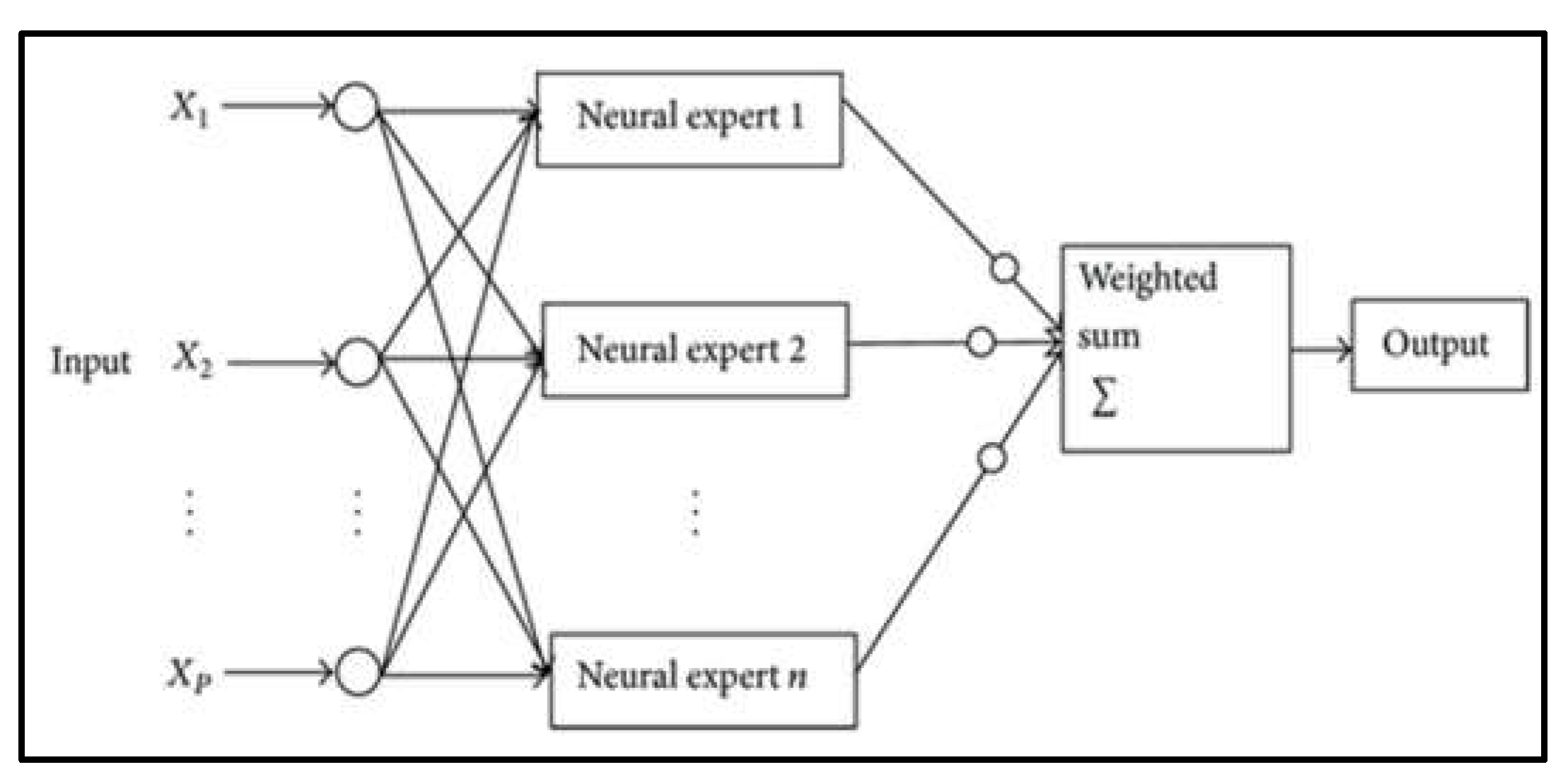
2.3. Developing the ANN Model

The artificial neural network is a data-based approach, different from conventional statistical methods. Therefore, a preliminary knowledge of the relationships among the input variables is not required in this case [42]. Furthermore, more reliable and robust relationships among the input and output parameters can be derived using the non-linear ANN models [43]. The published literature, although useful, is not all-encompassing, as far as the theory and methodology of ANN is concerned [42,44,45]. For this particular study, the ANN models employed to predict the impact of tractor speed on soil compaction using cone penetrologger test results were built by taking recourse to the Neuro Solutions software [46]. The used data for the calibration and the validation of the model included the penetration resistance data (CPR in other words) obtained from an electronic penetrologger. The model was developed using the steps outlined by the authors of [47]—identification of the relevant inputs and outputs, data division, architecture selection, optimization, validation, and model performance measurement.

2.4. Selection of Relevant Model Inputs/Outputs

In geotechnical engineering research, it is often common to rely on what is known about the system at the time of conducting the research—current knowledge, in other words. This is true for the analysis conducted by the authors of this paper as well. These input/output variables are selected in such a way as to include all the major factors that impact soil compaction.

Soil water content, bulk density, tractor forward speed, and other relevant soil characteristics. In this study, the electronic penetrologger measured the mean vertical stress necessary for cone penetration. This method provides the soil penetration resistance (CPR) output expressed in Nm⁻² or MPa. Moisture content is conjointly measured with the CPR data, as the latter is influenced by the former.

The Neuro Solutions software, which was used for this analysis, requires that one input node be allocated for every variable. The elaborated ANN models in the present study had a total of 4 input parameters consisting of 4 nodes, as listed hereunder:

(1)

Tractor speed (km/h);

(2)

Average depth below the ground surface, D (cm);

(3)

Soil bulk density (g/cm³);

(4)

Soil moisture content (%).

The single output variable is the final CPR (MPa) at depth D after compaction.

2.5. Data Division and Pre-Processing

The training, cross-validating, and testing of the model utilized 50%, 30%, and 20%, respectively, of the dataset [37] from 1000 to 10,000 iterations for the ANN structure reconstruction. Validation is considered the best point of generalization since it aborts the training when an accretion is noticed in the error. Once the network is trained with a testing set to compare its output with the desired output, the model weights are fixed [46]. The statistical characteristics assessed in the current study involved the mean, minimum, maximum, standard deviation, and range. After generating the clusters, samples were randomly identified and allocated correspondingly to the three data subsets. Before the calibration, the data were pre-processed by scaling. All the parameters were scalable in the selective [0.1–0.9] range (refer to Equation (1)). However, after training, the outputs of the model were inverse scaled.

I_scaled = a + ((I_unscaled − A) (b − a))/(B − A)

(1)

where A and B are the minima and maxima, respectively, of the unscaled dataset. Likewise, a and b are the minima and maxima of the scaly dataset.

To improve the ANN generalization ability, inputs and output data were normalized within the range 0–1 using Equation (2):

N = (X − X_min)/(X_max − X_min)

(2)

N is the normalized data; X is the measured value; and X_min and X_max are the minimum and maximum values, respectively.

2.6. Determination of Network Architecture

Modular feed forward (MFF) networks, MLPs (see Figure 3), used commonly for prediction and forecasting in geotechnical engineering [48], minimize the number of examples needed for the training without impacting the degree of accuracy [30].

The network geometry calls for identifying the numbers of hidden layers and nodes contained in each layer. Three layers including one hidden layer within the input and output layers [49,50] formed the MLP used in this research. According to [51], networks with one hidden layer and rather connection weights are capable of approaching any continuous function.

MLP is therefore able to capture the nonlinearity and complexity of the system by courtesy of the use of nonlinear activation functions in both the output and the hidden layers [52].

In order to achieve the optimum architecture, several ANN models were trained, starting with a single hidden layer neuron model and sequentially increasing the number of neurons to 11 [38]. In accordance with [5,53] and [38], the upper limit of hidden nodes necessary to map any continuous function for a network with I input nodes is equal to 2I + 1.

2.7. Model Optimization and Stopping Criterion

In an MFF neural network, the back-propagation algorithm is commonly adopted [1]. After the network is trained with a testing set to compare the output it yields with the desired output, the weights of the model are specified [5,53]. ANN performance should be evaluated using a validation dataset. Therefore, the optimum network is generated as soon as a rise in the test error is detected, presuming that the error area coincides with the overall minimum [1].

2.8. Model Validation and Performances Measures

The network is validated once the model has been optimized. The artificial neural network is envisaged to create non-linear relationships among the input and output parameters, instead of merely memorizing the forms that are outlined in the training data. Considering that the model is evaluated using a ‘hidden’ dataset, the results are substantial for the network performance evaluation [32]. The predictive performance was tested and compared using the determination coefficient (R²); the mean squared error (MSE); the mean absolute error (MAE); the % error; the Akaike information criterion (AIC); and the MDL criterion (minimum description length), which is similar to the AIC [38]. The goal is to minimize the AIC and MDL terms to build a network with the best generalization. MAE offers information on the error magnitude. The coefficient of correlation (R) determines the correlation between the measured and predicted data [1,5].

$$MSE=\frac{1}{n}{\displaystyle \sum _{i=1}^n(R_D}-R_P{)}^2$$

(3)

$$AIC(k)=n\log (MSE)+2k$$

(4)

$$MDL(k)=n\log (MSE)+0.5k\log (n)$$

(5)

$$R^2=\frac{RSS}{TSS}$$

(6)

where n is the number of exemplars of the training set; R_D and R_P are the measured and predicted values of penetration resistance, respectively; and k is the number of network weights. RSS and TSS coefficients present the sum of squares and the total sum of squares, respectively:

$$RSS={\displaystyle \sum _{i=1}^n(f_i}-\overline{f}{)}^2$$

(7)

$$TSS={\displaystyle \sum _{i=1}^n(Y_i}-\overline{Y}{)}^2$$

(8)

where $\overline{f}$ and $\overline{Y}$ are the means of the predicted values ($f_i$) and observed data ($Y_i$), respectively.

ǀRǀ > 0.8: a strong correlation exists between two sets of variables; 0.2 < ǀRǀ < 0.8: a correlation exists between two sets of variables; and ǀRǀ < 0.2: a weak correlation exists between two sets of variables [41].

2.9. Global Sensitivity Analysis

A sensitivity analysis of the selected optimum network was performed to identify the relative importance of the factors that are significant to improving predictions. The algorithm of [53] was used in this work, which partitions the network’s connection weights to define the relative importance of each input variable, just as many other researchers using this method have done earlier [32,34]. The sensitivity analysis was carried out twice with the connection weights obtained from the optimum ANN model that was ‘trained’ with 2 different models incorporating 2 hidden nodes.

3. Results and Discussion

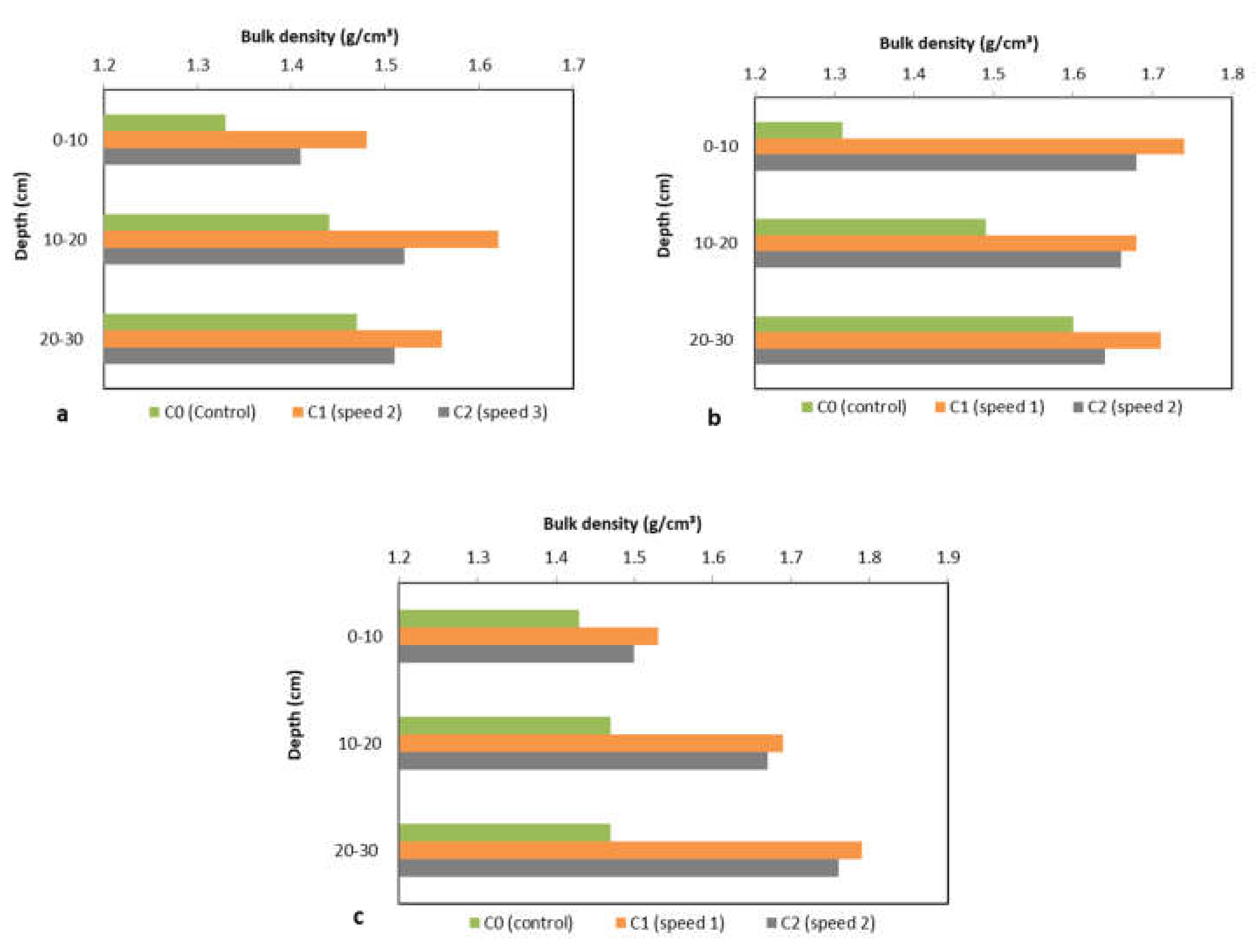
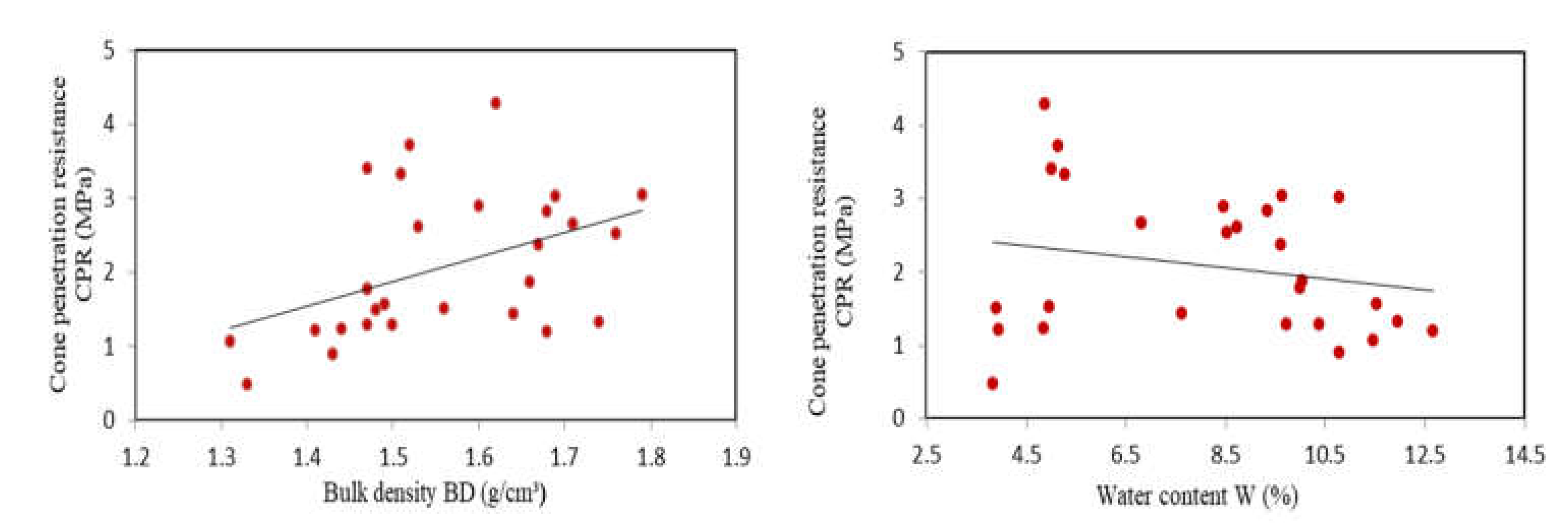
3.1. Bulk Density

It was noticed that the degree of soil compaction and the moisture content significantly affected the bulk density. The higher impact of tractor speed was noticed in the topsoil (Figure 4), which indicated that the subsoil was not as much affected as the topsoil. At lower speeds, the density increased up to a depth of 0–20 cm of the topsoil, but at depths greater than 20 cm, variation in the speeds did not result in any perceptible difference [8]. However, under the initial soil conditions (C0) and humidity H0, dry bulk density was already 1.33, 1.44, and 1.47 g/cm³ for layers 0–10, 10–20, and 20–30 cm, respectively. Statistical analysis (

Table 1. Comparison of bulk density BD (g/cm³) for different tillage horizons (cm) and speeds (km/h).

	Horizons	C0	C1	C2
H0	0–10	1.33 ± 0.05 a,A	1.48 ± 0.09 a,A,	1.41 ± 0.03 a,A
	10–20	1.44 ± 0.45 a,A	1.62 ± 0.05 a,B	1.52 ± 0.007 a,A,B
	20–30	1.47 ± 0.08 a,A	1.56 ± 0.10 a,A	1.51 ± 0.010 a,A
H1	0–10	1.31 ± 0.07 a,A	1.64 ± 0.01 a,B	1.68 ± 0.03 a,B
	10–20	1.49 ± 0.09 a,b,A	1.68 ± 0.14 a,A	1.66 ± 0.05 a,A
	20–30	1.6 ± 0.14 b,A	1.71 ± 0.18 a,A	1.64 ± 0.11 a,A
H2	0–10	1.46 ± 0.04 a,A	1.53 ± 0.06 a,A	1.5 ± 0.03 a,A
	10–20	1.47 ± 0.12 a,A	1.67 ± 0.06 a,b,A	1.67 ± 0.03 a,b,A
	20–30	1.47 ± 0.06 a,A	1.79 ± 0.07 b,B	1.76 ± 0.15 b,B

C0: no compaction, C1: speed 1 = 4 km h⁻¹, C2: speed 2 = 9 km h⁻¹, H0: initial water content = 4.6%, H1: water content after 15 days = 10%, H2: water content after 30 days = 9.8%, ±: standard deviation; the numbers followed by a common letter are not statistically different (p < 0.05): ^a,b: comparison of the horizons for the same modality, ^A,B: comparison of speeds by layer.

) of the obtained results revealed a significant impact of the tractor speed on soil bulk density (p < 0.05) for different depths and moisture contents. Increases in soil bulk density caused by the speed of tractor passages were observed to be higher at lower tractor speeds. In fact, for C1, the topsoil bulk density increased by 21%. In general, the soil bulk density increased with depth for all the treatments.

As soil moisture content increased, the effect of tractor speed on soil bulk density was greater, as has also been concluded by the authors of [54,55,56]. It can be generalized, in concert with [12], that tractor speed is an important determinant of soil compaction. There are studies [57] that have shown that a ‘cumulative compaction effect’ is observed with increasing speeds of passage.

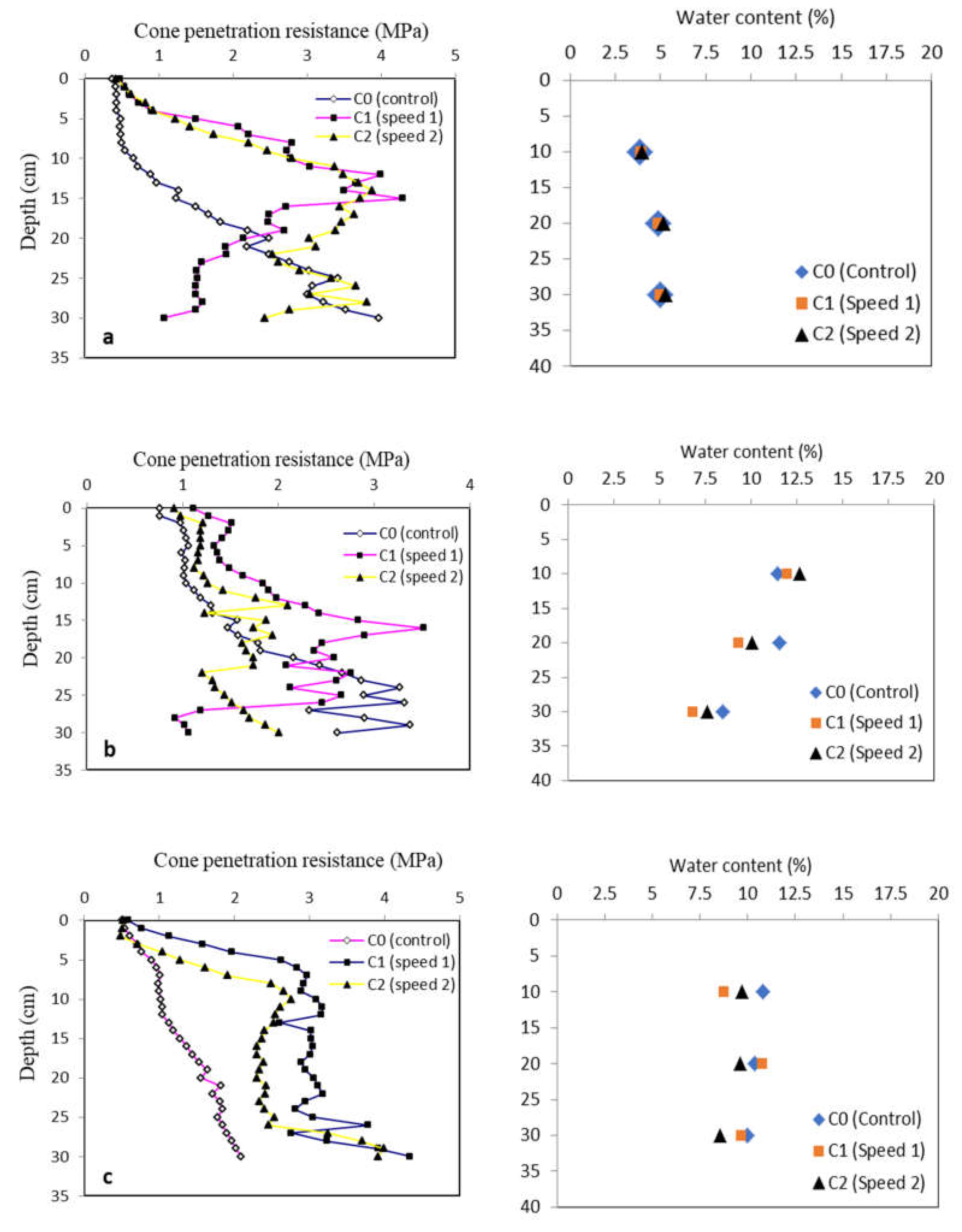
3.2. Cone Resistance to Penetration

Penetration resistance (CPR) data, as illustrated in Figure 5, showed a normal distribution. As reported by several studies [39,58,59,60], quite intuitively, CPR increases with an increase in the soil bulk density. The effect of tractor speed on CPR was significant (p < 0.01) for the topsoil (

Table 2. Comparison of penetration resistance (CPR) (in MPa) for different tillage horizons (cm) and speeds (km/h).

	Horizons	C0	C1	C2
H0	0–10	0.48 ± 0.01 a,A	1.5 ± 0.3 a,B	1.22 ± 0.2 a,B
	10–20	1.23 ± 0.02 b,A	4.29 ± 0.1 b,C	3.71 ± 0.03 c,B
	20–30	3.41 ± 0.01 c,C	1.52 ± 0.02 a,A	3.32 ± 0.04 b,B
H1	0–10	1.06 ± 0.02 a,A	1.33 ± 0.05 a,C	1.19 ± 0.03 a,B
	10–20	1.57 ± 0.03 b,A	2.83 ± 0.04 c,C	1.87 ± 0.1 c,B
	20–30	2.89 ± 0.1 c,C	2.66 ± 0.01 b,B	1.44 ± 0.05 b,A
H2	0–10	0.9 ± 0.2 a,A	2.62 ± 0.06 a,C	1.28 ± 0.03 a,B
	10–20	1.28 ± 0.04 a,A	3.02 ± 0.02 b,C	2.37 ± 0.03 b,B
	20–30	1.78 ± 0.2 b,A	3.04 ± 0.04 b,C	2.53 ± 0.05 c,B

C0: no compaction, C1: speed 1 = 4 km h⁻¹, C2: speed 2 = 9 km h⁻¹, H0: initial water content = 4.6%, H1: water content after 15 days = 10%, H2: water content after 30 days = 9.8%, ±: standard deviation; the numbers followed by a common letter are not statistically different (p < 0.05): ^a,b,c: comparison of the horizons for the same modality, ^A,B,C: comparison of speeds by layer.

). Comparison of CPR data at different speeds and layers for different soil conditions confirmed that the largest difference in the PR, among the treatments, was observed in the top 15 cm as for difference in the BD, where it was substantially higher for C1 (4 km h⁻¹) than for C0 and C2 (9 km h⁻¹) under the 10% water content. At 5 cm depth, the PR values were 0.48, 1.5, and 1.22 MPa, respectively, for treatments C0, C1, and C2, in dry conditions. At a depth of 15 cm, these values rose to 1.23, 4.29, and 3.71 MPa, respectively. The results obtained in this paper are not very different from the ones reported by the authors of [54], who concluded, inter alia, that an increase of approximately 221% in the tractor speed caused a drop in the cone index by 15% in both dry and wet conditions. It was observed that at a tractor speed of 9 km per hour, the degree of soil compaction was the lowest when the moisture content was 4.6%. The compaction of the topsoil was more perceptible, in comparison to soil at depths greater than 20 cm.

3.3. Prediction of Penetration Resistance PR

3.3.1. Descriptive Statistics

The summary of statistical characteristics of the data in the prediction of PR is presented in

Table 3. Residual analysis for the ANN model developed by the authors.

Model Variable	Minimum	Maximum	Mean	Median	SD	Skewness	Kurtosis
BD (g/cm3)	1.24	1.92	1.56	1.56	0.146	0.239	−0.324
W (%)	3.51	13.59	8.14	9.05	3.094	−0.101	−1.585
Speed (km/h)	0.00	9.00	4.33	4.000	4.509	0.330	−1.65
Depth (cm)	10	30	20	20	8.215	5.691 × 10−15	−1.518
CPR (MPa)	0.47	4.39	2.09	1.78	0.977	0.443	−0.801

.

Bulk density BD values varied between 1.24 and 1.92 g/cm³ (with an average value of 1.56 g/cm³)—a key finding of the electronic penetrologger tests. An already high soil BD at the outset may lead to a higher degree of soil compaction. The speeds tested ranged between 0 km/h (control, no compaction) and 9 km/h (with an average value of 4.33 km/h). ANN facilitates interpolation within the data fed into the model but is not used for extrapolation. Figure 6 shows the scatter plot relations among the PR and input data. The effects of speed, bulk density, and water content on penetration resistance are non-linear and complex, as is shown.

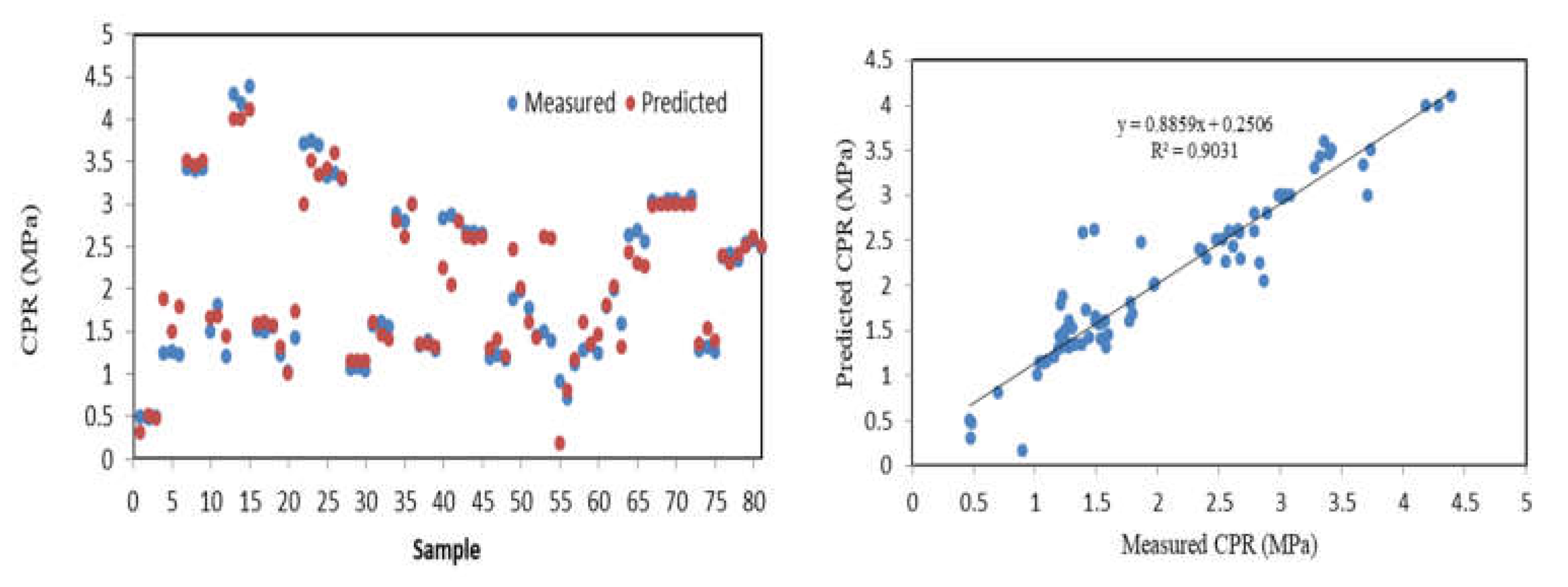
3.3.2. Results of the Optimal ANN Model

Several neurons and epochs were assessed by trial and error in order to find the best (optimum) ANN configuration for predicting the CPR (

Table 4. Performance of the optimal network with a single hidden layer and two nodes in a hidden layer.

		1. Speed
Input layer Hidden layer Output layer	Co-Variables	2. Depth
		3. Bulk density
		4. Moisture content
	Number of neurons	4
	Resizing method for covariates	Adjusted normalized
	Number of hidden layer/s	1
	Number of neurons in hidden layer	2
	Activation function	Hyperbolic tangent
	Dependent variable/s	1 CPRnce
	Number of neuron/s	1
	Resizing method for dependent scale variables	Standardized
	Error function	Sum of squares

). The ANN configuration regarded to be optimal should minimize the MSE value and the percentage error, as well as optimize R² [60]. The optimal ANN configuration from the network construction employed a single hidden layer, with two nodes in the upper and lower levels. The percentage error for this optimal configuration was 0.484 (

Table 5. Performance statistics of the optimum ANNs with single and two hidden layers.

Model	Activation Function	MSE	% Error	R
Single hidden layer model	TANH	0.056	0.484	0.95
Two hidden layer model	TANH	0.047	0.406	0.96

). The single optimum model and two hidden-layer models were compared among themselves for the accuracy of the predictions they could make. The two hidden-layer models registered a negligible improvement in performance (MSE difference of 0.009, percentage error equal to 0.078%, and difference in correlation R equal to 0.01). Therefore, the single hidden layer model was chosen. The model facilitates the expression of the relationship among the input and output variables as simple numerical equations.

The results shown in Figure 7 point to a robust agreement between the predicted and the measured values of CPR (R² = 0.90).

However, the impact of input data errors, operator errors committed during testing, shortcomings of equipment used, and unavoidable procedural errors on the performance of the ANN model must not be overlooked or wished away [1,61,62].

3.3.3. MLP-Based Numerical Equation

To simplify the propagation and implementation of the optimum MLP model, an adequately simple equation was established for predicting the impact of tractor speed on soil compaction using cone penetrologger test results. The optimum structure is presented in Figure 8, and the associated weights and biases are shown in

Table 6. Weights and minimum levels for the optimum ANN model.

Hidden Layer Node	Weight from Node i in Input Layer to Node j in Hidden Layer (wji)				Hidden Layer Threshold (ɵj)
	i = 1	i = 2	i = 3	i = 4
j = 5	−0.137	0.218	−0.302	−0.292	−0.277
j = 6	0.404	1.050	0.728	−0.656	0.238
Output Layer Node	Weight from Node j in Hidden Layer to Node k in Output (wkj)				Hidden layer Threshold (ɵk)
	j = 5		j = 6
k = 7	−0.007		0.748		−0.218

. Equation (9) shows the mathematical relation between the input and output variables.

$${\mathrm{O}}_{\mathrm{K}}={ʄ}_{\tanh }\{{\mathrm{ɵ}}_{\mathrm{k}}+{\sum }_{\mathrm{j}=5}^6{\mathrm{W}}_{\mathrm{k}\mathrm{j}}{ʄ}_{\tanh }[{\mathrm{ɵ}}_{\mathrm{j}}+{\sum }_{\mathrm{i}=1}^4\left({\mathrm{W}}_{\mathrm{j}\mathrm{i}}{\mathrm{I}}_{\mathrm{i}}\right)]\}$$

(9)

where O_K is the single output variable, the final CPR (MPa) at depth D below the ground; θ_k is the threshold value at the output layer, and w_kj is the connection weight between the jth neuron in the hidden layer and the kth neuron in output layer; θ_j is the minimum value of the jth hidden neuron, and w_ji is the connection weight between the ith input neuron and the jth hidden neuron; Ii is the ith input parameter; and ʄ_tanh is the hyperbolic tangent function.

Equation (10) can be further simplified as follows:

$${\mathrm{T}}_{\mathrm{j}=5,6}=\frac{1}{1+\exp \{-\lfloor ɵj+\sum _{i=1}^4\{\mathrm{w}\mathrm{j}\mathrm{i}I\mathrm{i}\rfloor \}}$$

(10)

$${\mathrm{O}}_{\mathrm{K}=7}=\frac{1}{1+\exp \{-\lfloor ɵ\mathrm{k}+\sum _{\mathrm{j}=5}^6\{\mathrm{w}\mathrm{k}\mathrm{j}\mathrm{T}\mathrm{j}\rfloor \}}$$

(11)

The variables I1, I2, I3, and I4 represent the forward tractor speed, soil depth, soil bulk density, and water content, respectively. These four input parameters are described with the aid of a binary representation, in which ‘0′ and ‘1′ stand for their absence and presence, respectively. In particular, the use of the numerical equation (Equation (12)) for the tractor speed, I1, is taken as unity. The remaining input variables, given by I2, I3, and I4, represent the average depth (D), the soil bulk density (BD), and the cone penetration resistance (CPR), respectively. Nevertheless, the input and output parameters need to be scaleable before being used in the Equations (12)–(14). This is done using Equation (1), scaled between 0.1 and 0.9, in accordance with the minima and maxima of the data used in the training set. The connection weights (w_ji and w_kj), as well as the threshold levels (θ_j and θ_k), used in Equations (13) and (14) are sourced from Table 5. Therefore, the mathematical relationship for the optimum model including two hidden neurons is presented as follows:

$$\mathrm{CPR}=\frac{1}{1+\exp (0.007T5-0.748T6+0.218)}$$

(12)

where

$${\mathrm{T}}_{5 }={\left[1+\exp \left(0.137\mathrm{I}1-0.218\mathrm{I}2+0.302\mathrm{I}3+0.292\mathrm{I}4+0.277\right)\right]}^{-1}$$

(13)

$${\mathrm{T}}_{6 }={\left[1+\exp \left(-0.404\mathrm{I}1-1.050\mathrm{I}2-0.728\mathrm{I}3+0.656\mathrm{I}4-0.238\right)\right]}^{-1}$$

(14)

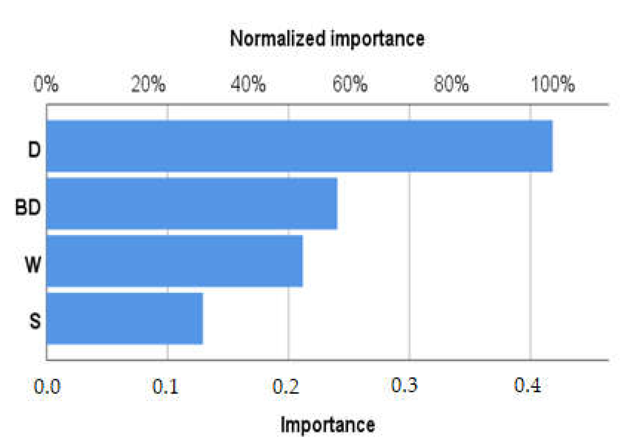
3.3.4. Selection of Significant Input Parameters

The relative importance of the variables in the improvement of prediction accuracy can be determined by performing a sensitivity analysis [61,62]. According to [60,63], the algorithm employed in the current study divides the connection weights of the network to set the relative importance of each input variable.

Figure 9 shows that there is a significant correlation between the input variables and the penetration resistance (PR). It can be proven that the most significant predictor variable is the depth below the soil surface D (42% of importance), followed by the soil bulk density BD (24%) and W (21%). The least significant parameter is the tractor speed (13%). In fact, BD impacts the available soil moisture content, movement of water and air in the soil, and the development of the roots of the crops. Bulk density thus is an important indicator of soil compaction, and thereby the resistance offered by the soil to penetration [5]. As BD increases, the PR increases along with it, affecting crop yields, and by decreasing the vegetative cover, hastens soil erosion. Understanding the relationship among BD, W, and PR is thereby of great interest and importance.

4. Conclusions

In this study, the effects of a set of variables—tractor speed, soil moisture content, bulk density, and average depth below the ground surface—on the degree of soil compaction were analyzed for alluvial, poorly developed soil samples collected in Tunisia. Among other findings, it was observed that at a tractor speed of 4 km per hour, the degree of soil compaction was the highest for higher moisture content. The compaction of the topsoil was more perceptible compared to soil at depths greater than 20 cm. Within the framework of the experimental setup, it can be concluded that the speed of the tractor did have a bearing on the degree of compaction of the topsoil, while soil depth and bulk density of the topsoil were the dominant parameters, as shown by the sensitivity analysis. At lower speeds, there was a conspicuous increase in the bulk density (of the topsoil, up to a depth of 15 cm) and thereby in the penetration resistance offered by it. The results posit the ANN model as an effective tool that can be used for accurately predicting (R value 0.95, MSE value 0.056) the degree of soil compaction (which, as has been pointed out earlier, results in a host of environmental and agronomic problems), contributing a numerical equation that can be used by geotechnical engineers in the future.

References

1. Ranasinghe, R.; Jaksa, M.; Kuo, Y.; Nejad, F.P. Application of artificial neural networks for predicting the impact of rolling dynamic compaction using dynamic cone penetrometer test results. J. Rock Mech. Geotech. Eng. 2017, 9, 340–349. [Google Scholar] [CrossRef] [Green Version]
2. Guengant, J.P.; May, J. Africa 2050: African Demography; Emerging Markets Forum: Washington, DC, USA, 2013; p. 60. [Google Scholar]
3. Jaksa, M.B.; Scott, B.T.; Mentha, N.L.; Symons, A.T.; Pointon, S.M.; Wrightson, P.T.; Syamsuddin, E. Quantifying the zone of influence of the impact roller. In Proceedings of the ISSMGETC International Symposium on Ground Improvement, Brussels, Belgium, 31 May–1 June 2012. [Google Scholar]
4. Oldeman, L.R. Global Extent of Soil Degradation; Bi-Annual Report; ISRIC: Wageningen, The Netherlands, 1991–1992; pp. 19–36. [Google Scholar]
5. Abrougui, K.; Gabsi, K.; Mercatoris, B.; Khemis, C.; Amami, R.; Chehaibi, S. Prediction of organic potato yield using tillage systems and soil properties by artificial neural network (ANN) and multiple linear regressions (MLR). Soil Tillage Res. 2019, 190, 202–208. [Google Scholar] [CrossRef]
6. Lull, H.W. Soil Compaction on Forest and Range Lands; Forest Service, US Department of Agriculture: Washington, DC, USA, 1959.
7. Soane, B.; van Ouwerkerk, C. Implications of soil compaction in crop production for the quality of the environment. Soil Tillage Res. 1995, 35, 5–22. [Google Scholar] [CrossRef]
8. Alakukku, L.; Peter Weisskopf, W.C.T.; Chamen, F.G.J.; Tijink, J.P.; van der Linden, S.; Pires, C.; Sommer, G. Prevention strategies for field traffic-induced subsoil compaction: A review: Part 1. Machine/soil interactions. Soil Tillage Res. 2003, 73, 145–160. [Google Scholar] [CrossRef]
9. Alaoui, A.; Lipiec, J.; Gerke, H. A review of the changes in the soil pore system due to soil deformation: A hydrodynamic perspective. Soil Tillage Res. 2011, 115–116, 1–15. [Google Scholar] [CrossRef]
10. Nawaz, M.F.; Bourrié, G.; Trolard, F. Soil compaction impact and modelling. A review. Agron. Sustain. Dev. 2012, 33, 291–309. [Google Scholar] [CrossRef] [Green Version]
11. Charreau, C.J. Problems posed by agricultural use of tropical soils by annual crops. Tropical Agronomy. Series 2, General Agronomy. Technical Studies. 27, 905–929. Conference on Soil Fertility, Ibadan, Nigeria. 1972. Available online: https://agritrop.cirad.fr/435651/ (accessed on 9 May 2022).
12. Kayombo, B.; Lal, R. Responses of Tropical Crops to Soil Compaction; Elsevier: Amsterdam, The Netherlands, 1994; pp. 287–316. [Google Scholar] [CrossRef]
13. Jabro, J.D.; Iversen, W.M.; Evans, R.G.; Allen, B.L.; Stevens, W.B. Repeated Freeze-Thaw Cycle Effects on Soil Compaction in a Clay Loam in Northeastern Montana. Soil Sci. Soc. Am. J. 2014, 78, 737–744. [Google Scholar] [CrossRef]
14. Cohron, G. Forces Causing Soil Compaction; Compaction of Agricultural Soils; FAO, AGRIS: Rome, Italy, 1971; pp. 106–122. [Google Scholar]
15. Greene, W.D.; Stuart, W.B. Skidder and Tire Size Effects on Soil Compaction. South. J. Appl. For. 1985, 9, 154–157. [Google Scholar] [CrossRef]
16. Schjønning, P.; van den Akker, J.; Keller, T.; Greve, M.; Lamandé, M.; Simojoki, A.; Stettler, M.; Arvidsson, J.; Breuning-Madsen, H. Driver-pressure-state-impact-response (DPSIR) analysis and risk assessment for soil compaction-a European perspective. Adv. Agron. 2015, 133, 183–237. [Google Scholar]
17. Ren, L.; D’Hose, T.; Ruysschaert, G.; de Pue, J.; Meftah, R.; Cnudde, V.; Cornelis, W.M. Effects of soil wetness and tyre pressure on soil physical quality and maize growth by a slurry spreader system. Soil Tillage Res. 2019, 195, 104344. [Google Scholar] [CrossRef]
18. Horn, R.; Domżżał, H.; Słowińska-Jurkiewicz, A.; van Ouwerkerk, C. Soil compaction processes and their effects on the structure of arable soils and the environment. Soil Tillage Res. 1995, 35, 23–36. [Google Scholar] [CrossRef]
19. Destain, M.F. La Compaction des Sols Agricoles en Wallonie, SPW; Université de Liège, Gembloux Agro-Bio Tech: Liege, Belgium, 2014; p. 54. [Google Scholar]
20. Chamen, T.; Alakukku, L.; Pires, S.; Sommer, C.; Spoor, G.; Tijink, F.; Weisskopf, P. Prevention strategies for field traffic-induced subsoil compaction: A review: Part 2. Equipment and field practices. Soil Tillage Res. 2003, 73, 161–174. [Google Scholar] [CrossRef]
21. Hamza, M.A.; Anderson, W.K. Soil compaction in cropping systems: A review of the nature, causes and possible solutions. Soil Tillage Res. 2005, 82, 121–145. [Google Scholar] [CrossRef]
22. Arvidsson, J.; Keller, T. Soil stress as affected by wheel load and tyre inflation pressure. Soil Tillage Res. 2007, 96, 284–291. [Google Scholar] [CrossRef]
23. Sakai, H.; Nordfjell, T.; Suadicani, K.; Talbot, B.; Bollehuus, E. Soil compaction on forest soils from different kinds of tires and tracks and possibility of accurate estimate. Croat. J. For. Eng. 2008, 29, 15–27. [Google Scholar]
24. Barbosa, L.A.; Magalhães, P.S. Tire tread pattern design trigger on the stress distribution over rigid surfaces and soil compaction. J. Terramech. 2015, 58, 27–38. [Google Scholar] [CrossRef]
25. Khemis, C.; Abrougui, K.; Lidong, R.; Mutuku, E.A.; Chehaibi, S.; Cornelis, W. Effects of tractor loads and tyre pressures on soil compaction in Tunisia under different moisture conditions. In Proceedings of the 19th EGU General Assembly, EGU2017. Vienna, Austria, 23–28 April 2017; p. 15218. [Google Scholar]
26. Khodaei, M. Evaluation of corn planter under travel speed, working depth, pressure wheel and cone index. Agric. Eng. Int. CIGR J. 2015, 17, 73–80. [Google Scholar]
27. Horn, R.; Albrechts, C. Stress strain effects in structured unsaturated soils on coupled mechanical and hydraulic processes. In Proceedings of the 18th World Congress of Soil Science, Philadelphia, PA, USA, 9–15 July 2003. [Google Scholar]
28. Hamza, M.A.; Al-Adawi, S.; Al-Hinai, K.A. Effect of combined soil water and external load on soil compaction. Soil Res. 2011, 49, 135–142. [Google Scholar] [CrossRef]
29. Destain, M.-F.; Roisin, C.; Dalcq, A.-S.; Mercatoris, B. Effect of wheel traffic on the physical properties of a Luvisol. Geoderma 2016, 262, 276–284. [Google Scholar] [CrossRef]
30. Günaydın, O. Estimation of soil compaction parameters by using statistical analyses and artificial neural networks. Environ. Earth Sci. 2008, 57, 203–215. [Google Scholar] [CrossRef]
31. Isik, F.; Ozden, G. Estimating compaction parameters of fine- and coarse-grained soils by means of artificial neural networks. Environ. Earth Sci. 2012, 69, 2287–2297. [Google Scholar] [CrossRef]
32. Shahin, M.A.; Jaksa, M.B. Pullout capacity of small ground anchors by direct cone penetration test methods and neural networks. Can. Geotech. J. 2006, 43, 626–637. [Google Scholar] [CrossRef] [Green Version]
33. Kuo, Y.; Jaksa, M.; Lyamin, A.; Kaggwa, W. ANN-based model for predicting the bearing capacity of strip footing on multi-layered cohesive soil. Comput. Geotech. 2008, 36, 503–516. [Google Scholar] [CrossRef]
34. Nejad, F.P.; Jaksa, M.B.; Kakhi, M.; McCabe, B.A. Prediction of pile settlement using artificial neural networks based on standard penetration test data. Comput. Geotech. 2009, 36, 1125–1133. [Google Scholar] [CrossRef] [Green Version]
35. Varella, C.; Pinto, F.; Queiroz, D.M.; Sena, D.G. Determinacao da cobertura do solo poranalise de imagensdigitais e redesneurais. Rev. Bras. Eng. Agric. Ambient. 2002, 6, 225–229. (In Portuguese) [Google Scholar] [CrossRef] [Green Version]
36. Khazaei, J.; Daneshmandi, S. Modeling of thinlayer drying kinetics of sesame seeds: Mathematical and neural networks modeling. Int. Agrophys. 2007, 21, 335–348. [Google Scholar]
37. Sarmadian, F.; Mehrjardi, T.; Akbarzadeh, A. Modeling of some soil properties using artificial neural network and multivariate regression in Gorgan province, north of Iran. Aust. J. Basic Appl. Sci. 2009, 3, 323–329. [Google Scholar]
38. Trigui, M.; Gabsi, K.; El Amri, I.; Helal, A.; Barrington, S. Modular feed forward networks to predict sugar diffusivity from date pulp Part, I. Model validation. Int. J. Food Prop. 2011, 14, 356–370. [Google Scholar] [CrossRef]
39. Bouwman, L.; Arts, W. Effects of soil compaction on the relationships between nematodes, grass production and soil physical properties. Appl. Soil Ecol. 2000, 14, 213–222. [Google Scholar] [CrossRef]
40. Sharifi, A.; Godwin, R.J.; O’Dogherty, M.J.; Dresser, M.L. Evaluating the performance of a soil compaction sensor. Soil Use Manag. 2007, 23, 171–177. [Google Scholar] [CrossRef]
41. Keller, T.; Défossez, P.; Weisskopf, P.; Arvidsson, J.; Richard, G. SoilFlex: A model for prediction of soil stresses and soil compaction due to agricultural field traffic including a synthesis of analytical approaches. Soil Tillage Res. 2007, 93, 391–411. [Google Scholar] [CrossRef]
42. Shahin, M.A. State-of-the-art review of some artificial intelligence applications in pile foundations. Geosci. Front. 2016, 7, 33–44. [Google Scholar] [CrossRef] [Green Version]
43. Onoda, T. Neural network information criterion for the optimal number of hidden units. In Proceedings of the International Conference on Neural Networks, Perth, Australia, 27 November–1 December 1995; pp. 275–280. [Google Scholar]
44. Hecht-Nielsen, R. Theory of the backpropagation neural network. In Proceedings of the International Joint Conference on Neural Networks (IJCNN), Washington, DC, USA, 6 August 1989; pp. 593–605. [Google Scholar]
45. Ripley, B.D. Neural Networks and Related Methods for Classification. J. R. Stat. Soc. Ser. B 1994, 56, 409–437. [Google Scholar] [CrossRef]
46. NeuroDimension Inc. Neurosolutions Software; NeuroDimension Inc.: Gainesville, FL, USA, 2006. [Google Scholar]
47. Maier, H.R.; Jain, A.; Dandy, G.C.; Sudheer, K. Methods used for the development of neural networks for the prediction of water resource variables in river systems: Current status and future directions. Environ. Model. Softw. 2010, 25, 891–909. [Google Scholar] [CrossRef]
48. Kim, M.; Gilley, J.E. Artificial Neural Network estimation of soil erosion and nutrient concentrations in runoff from land application areas. Comput. Electron. Agric. 2008, 64, 268–275. [Google Scholar] [CrossRef] [Green Version]
49. Kowalczyk-Juśko, A.; Pochwatka, P.; Zaborowicz, M.; Czekała, W.; Mazurkiewicz, J.; Mazur, A.; Janczak, D.; Marczuk, A.; Dach, J. Energy value estimation of silages for substrate in biogas plants using an artificial neural network. Energy 2020, 202, 117729. [Google Scholar] [CrossRef]
50. Erzin, Y.; Rao, B.H.; Patel, A.; Gumaste, S.; Singh, D. Artificial neural network models for predicting electrical resistivity of soils from their thermal resistivity. Int. J. Therm. Sci. 2010, 49, 118–130. [Google Scholar] [CrossRef]
51. Cybenko, G. Approximation by superpositions of a sigmoidal function. Math. Control Signals Syst. 1989, 2, 303–314. [Google Scholar] [CrossRef]
52. Hornik, K.; Stinchcombe, M.; White, H. Multilayer feedforward networks are universal approximators. Neural Netw. 1989, 2, 359–366. [Google Scholar] [CrossRef]
53. Garson, D.G. Interpreting neural network connection weights. AI Expert. 1991, 6, 47–51. [Google Scholar]
54. Horn, R.; Rostek, J.J. Subsoil compaction processes-state of knowledge. Adv. Geoecol. 2000, 32, 44–54. [Google Scholar]
55. Arman, K. Tractor forward velocity and tire load effects on soil compaction. J. Terramech. 1994, 31, 11–20. [Google Scholar] [CrossRef]
56. Ansorge, D.; Godwin, R.J.B.E. The Effect of Tyres and a Rubber Track at High Axle Loads on Soil Compaction Part 2. Multi-Axle Machine Studies; Cranfield University: Cranfield, UK, 2008; pp. 338–347. [Google Scholar]
57. Etana, A.; Håkansson, I. Swedish experiments on the persistence of subsoil compaction caused by vehicles with high axle load. Soil Tillage Res. 1994, 29, 167–172. [Google Scholar] [CrossRef]
58. Taylor, H.M.; Throckmorton, R.I.; van den Berg, G.E. Compaction of Agricultural Soils; ASAE: St. Joseph, MI, USA, 1971; pp. 292–305. [Google Scholar]
59. Servadio, P.; Marsili, A.; Vignozzi, N.; Pellegrini, S.; Pagliai, M. Effects on some soil qualities in central Italy following the passage of four wheel drive tractor fitted with single and dual tires. Soil Tillage Res. 2005, 84, 87–100. [Google Scholar] [CrossRef]
60. Abdipour, M.; Younessi-Hmazekhanlu, M.; Ramazani, S.H.R. Artificial neural networks and multiple linear regression as potential methods for modeling seed yield of safflower 496 (Carthamus tinctorius, L.). Ind. Crops Prod. 2019, 127, 185–194. [Google Scholar] [CrossRef]
61. Kowalski, P.A.; Kusy, M. Determining significance of input neurons for probabilistic neural network by sensitivity analysis procedure. Comput. Intell. 2017, 34, 895–916. [Google Scholar] [CrossRef]
62. Mehmet, A.B.; Ehsan, H.; Mehmet, F.; Seyed, E.; Aghakouchaki, H.; Ercan, I. A Hybrid ANN-GA Model for an Automated Rapid Vulnerability Assessment of Existing RC Buildings. Appl. Sci. 2022, 12, 5138. [Google Scholar]
63. Sung-Sik, P.; Peter, O.; Seung-Wook, W.; Dong-Eun, L. A Simple and Sustainable Prediction Method of Liquefaction-Induced Settlement at Pohang Using an Artificial Neural Network. Sustainability 2020, 12, 4001. [Google Scholar]
Figure 2. Experimental design (C0: control, C1: speed1 = 4 km/h, C2: speed2 = 9 km/h) under three moisture conditions, H0: initial water content (4.6%), H1: water content after 15 days (10%), and H2: water content after 30 days (9.8%).
Processes 10 01109 g002
Figure 3. General construction of modular feed forward (MFF) network.
Processes 10 01109 g003
Figure 4. Bulk density for three level of compaction and different tractor speeds C0: control, C1: speed1 = 4 km h−1, C2: speed2 = 9 km h−1 under three moisture conditions: (a) H0: initial water content (4.6%); (b) H1: water content after 15 days (10%); (c) H2: water content after 30 days (9.8%). The same tractor was used for all the treatments with a tire inflation pressure of 1500 kg/cm2.
Processes 10 01109 g004
Figure 5. Penetration resistance (CPR) at different depths after C0: no compaction, C1: speed1 = 4 km h−1, C2: speed2 = 9 km h−1 under three moisture conditions: (a) H0: initial water content (4.6%), (b) H1: water content after 15 days (10%), (c) H2: water content after 30 days (9.8%) and corresponding soil water contents.
Processes 10 01109 g005
Figure 6. Scatter plot displaying between penetration resistance CPR and input dataset.
Processes 10 01109 g006
Figure 7. Predicted final CPR (MPa) for the optimal ANN model.
Processes 10 01109 g007
Figure 8. Configuration of the optimum MLP model.
Processes 10 01109 g008
Figure 9. Normalized and absolute importance of the input variables for the MLP artificial neural network with better performance.
Processes 10 01109 g009