
Improved Employee Safety Behavior Risk Assessment of the Train Operation Department Based on Grids

Abstract
:1. Introduction
2. Literature Review
3. Methodology
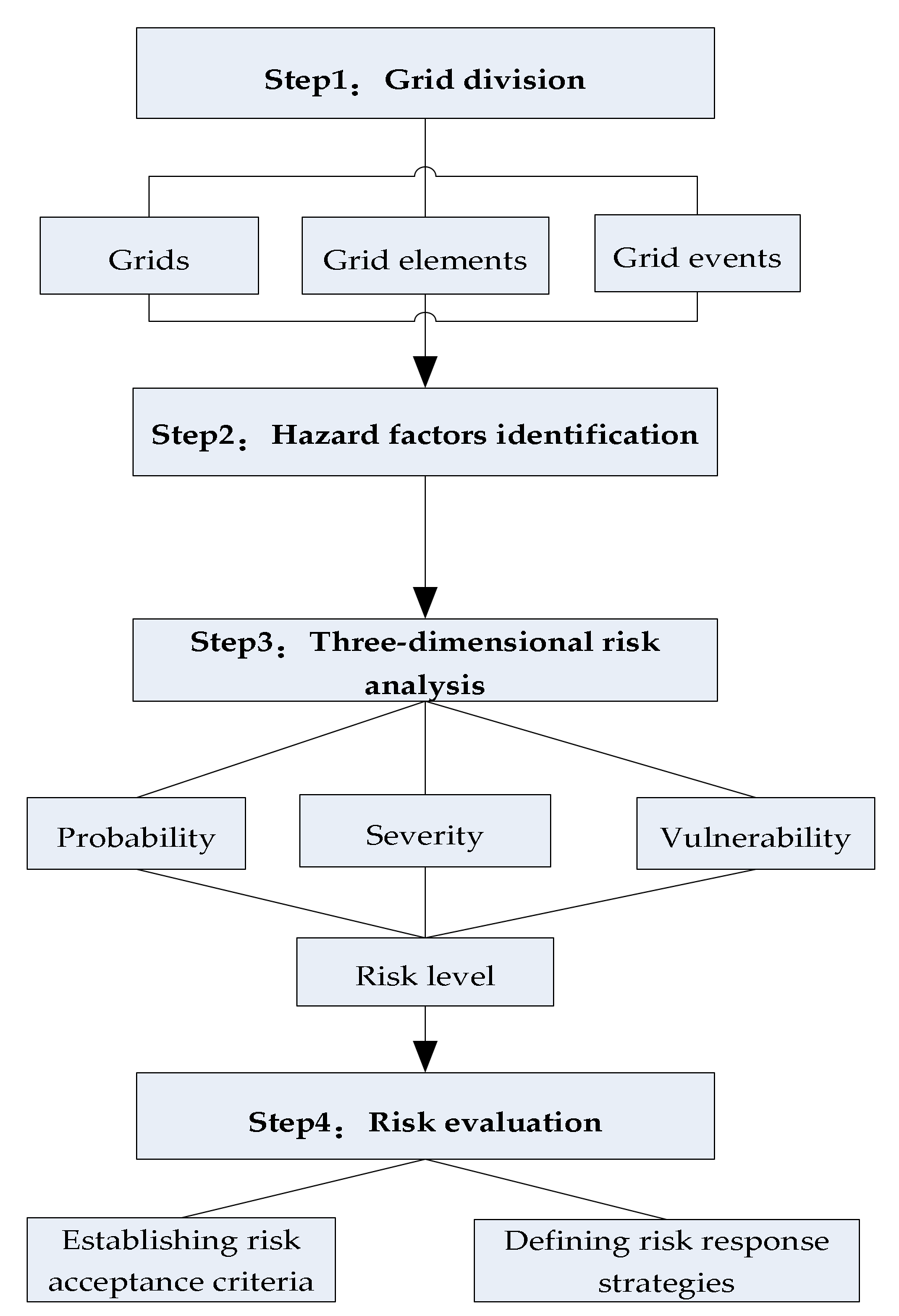
3.1. Proposed Framework
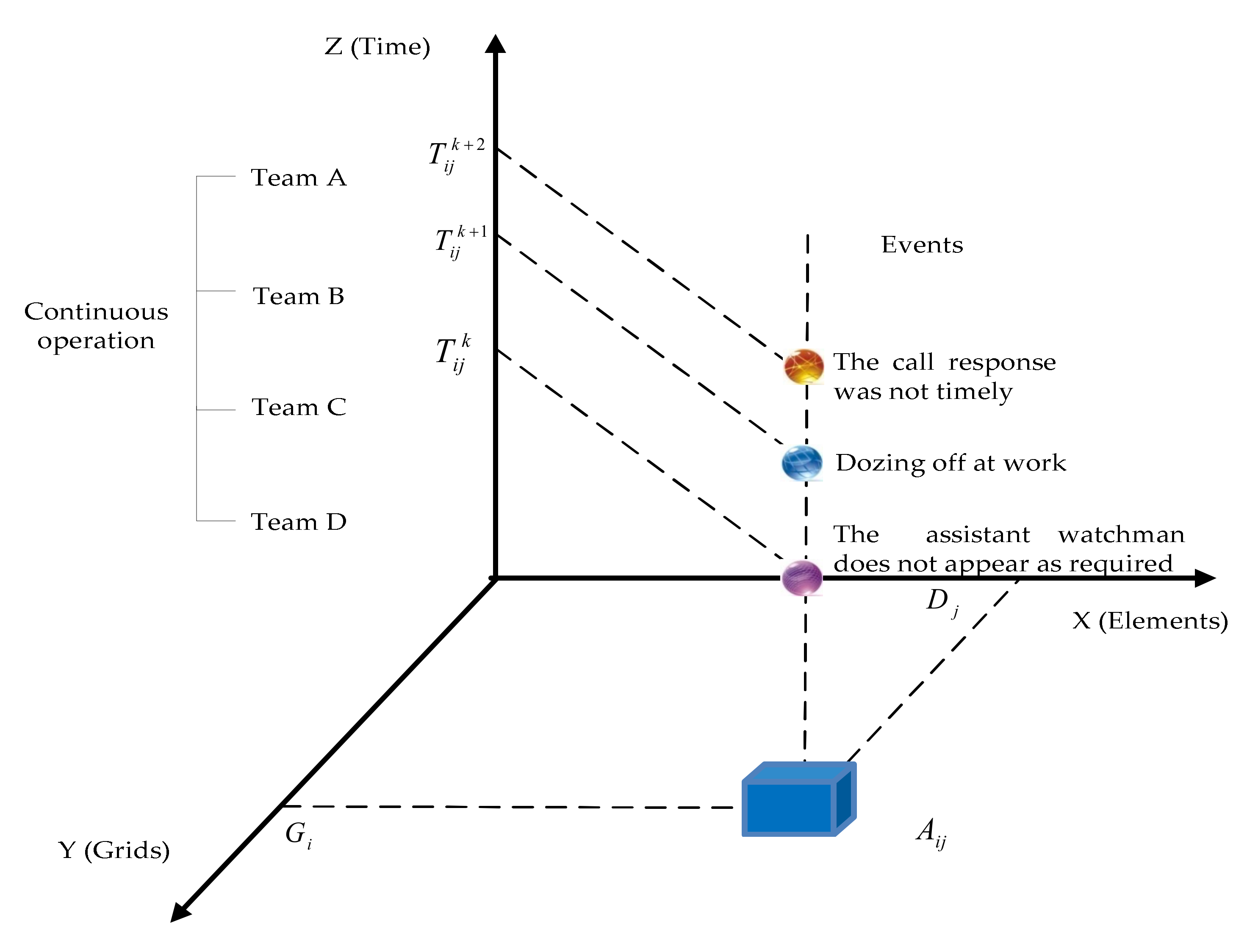
3.2. Grid Division
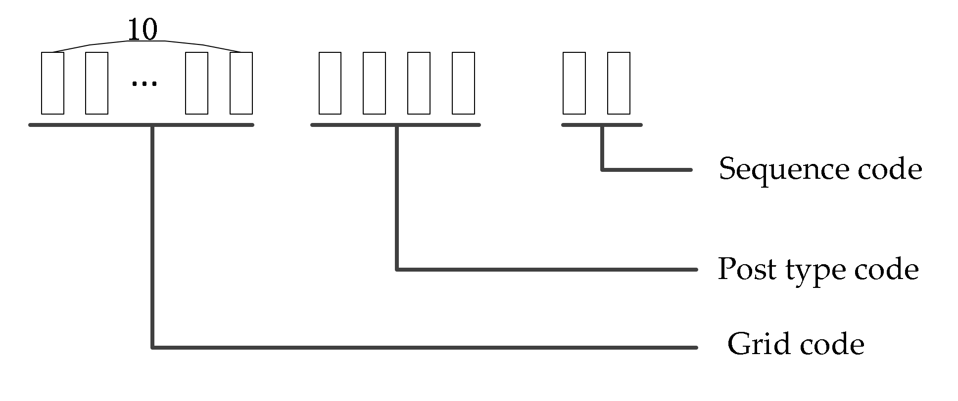
- (1)
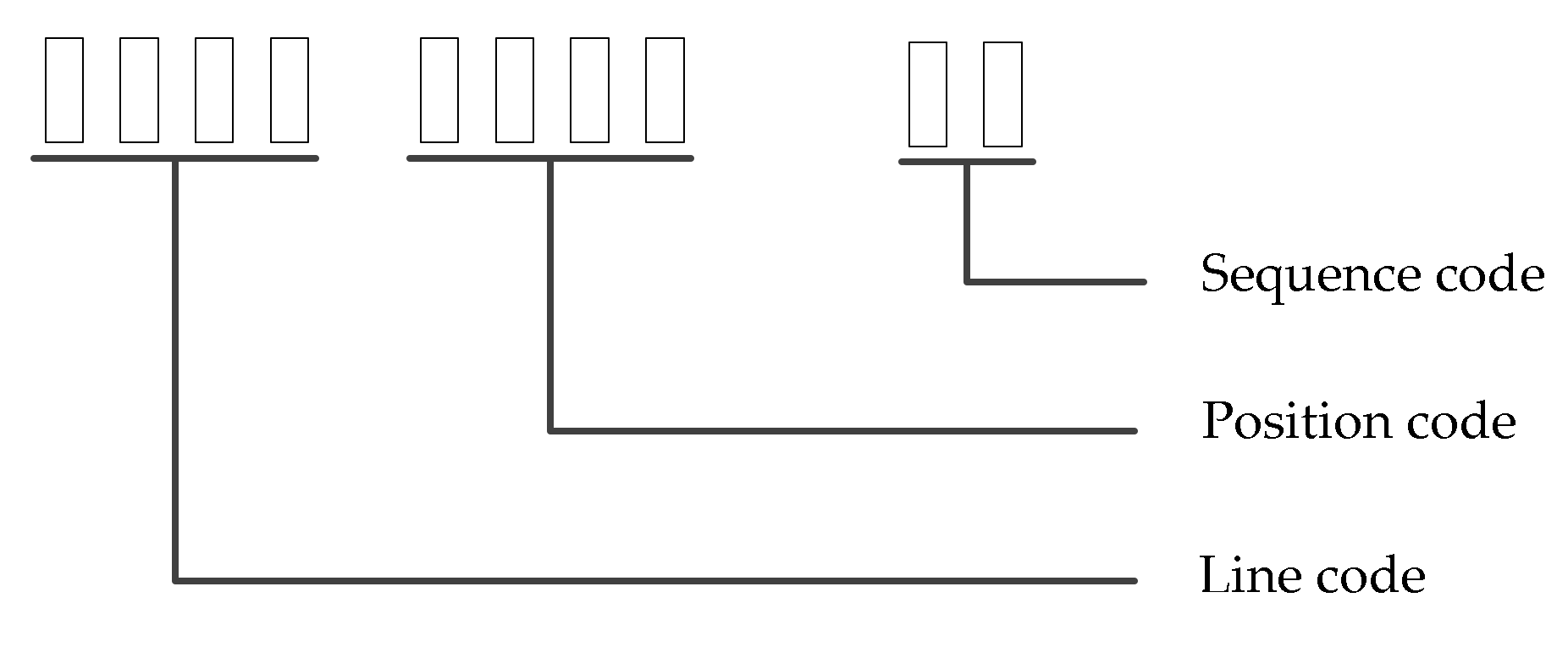
- Grid definition and coding
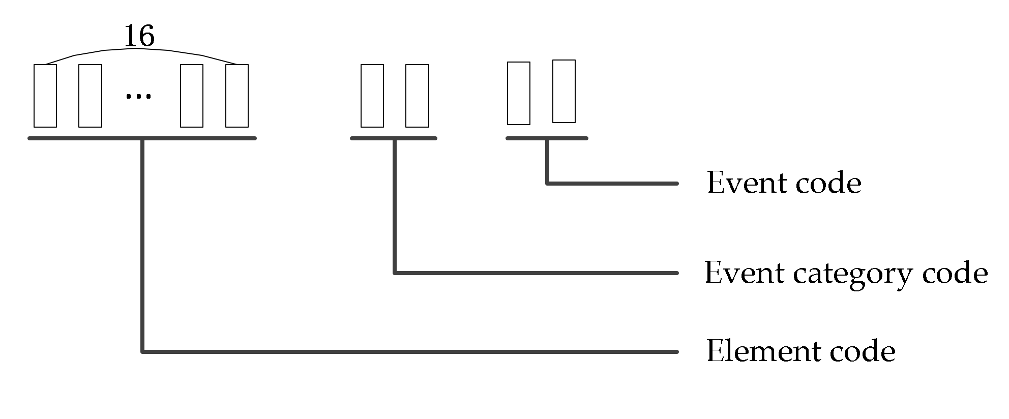
- (2)
- Definition and coding of grid elements
- (3)
- Definition and encoding of grid events
3.3. Hazard Factors Identification
3.4. Risk Analysis
- (1)
- Risk assessment criteria
- (2)
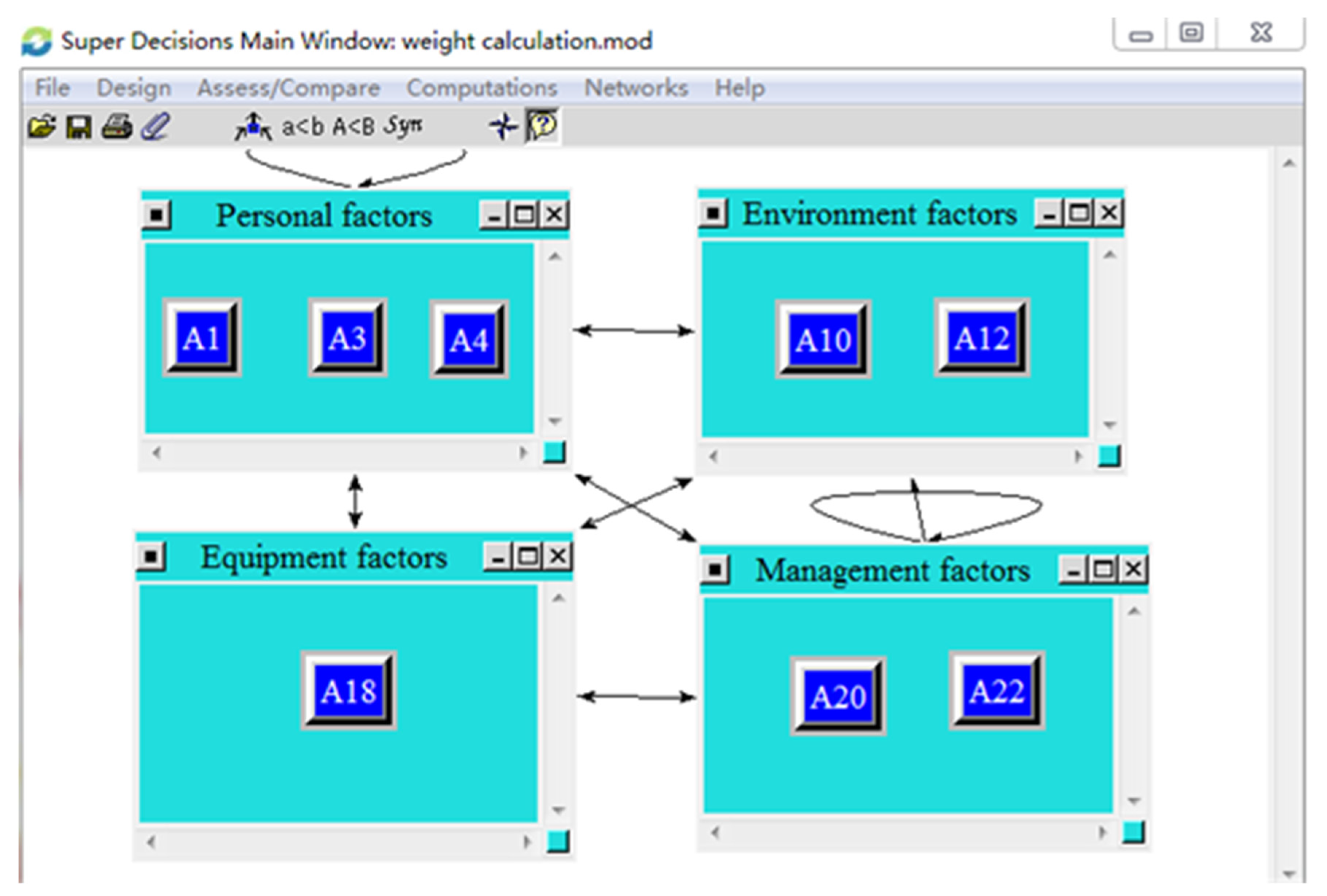
- Weights of the hazard factors
- (3)
- Probability calculation
- (4)
- Vulnerability calculation
- (5)
- Severity calculation
- (6)
- Risk level calculation
3.5. Risk Evaluation
- Risk response priorities;
- What approach should be taken to implement the selected response activities?
- Whether a response activity should be carried out;
- Whether a risk needs to be dealt with.
4. Case Study
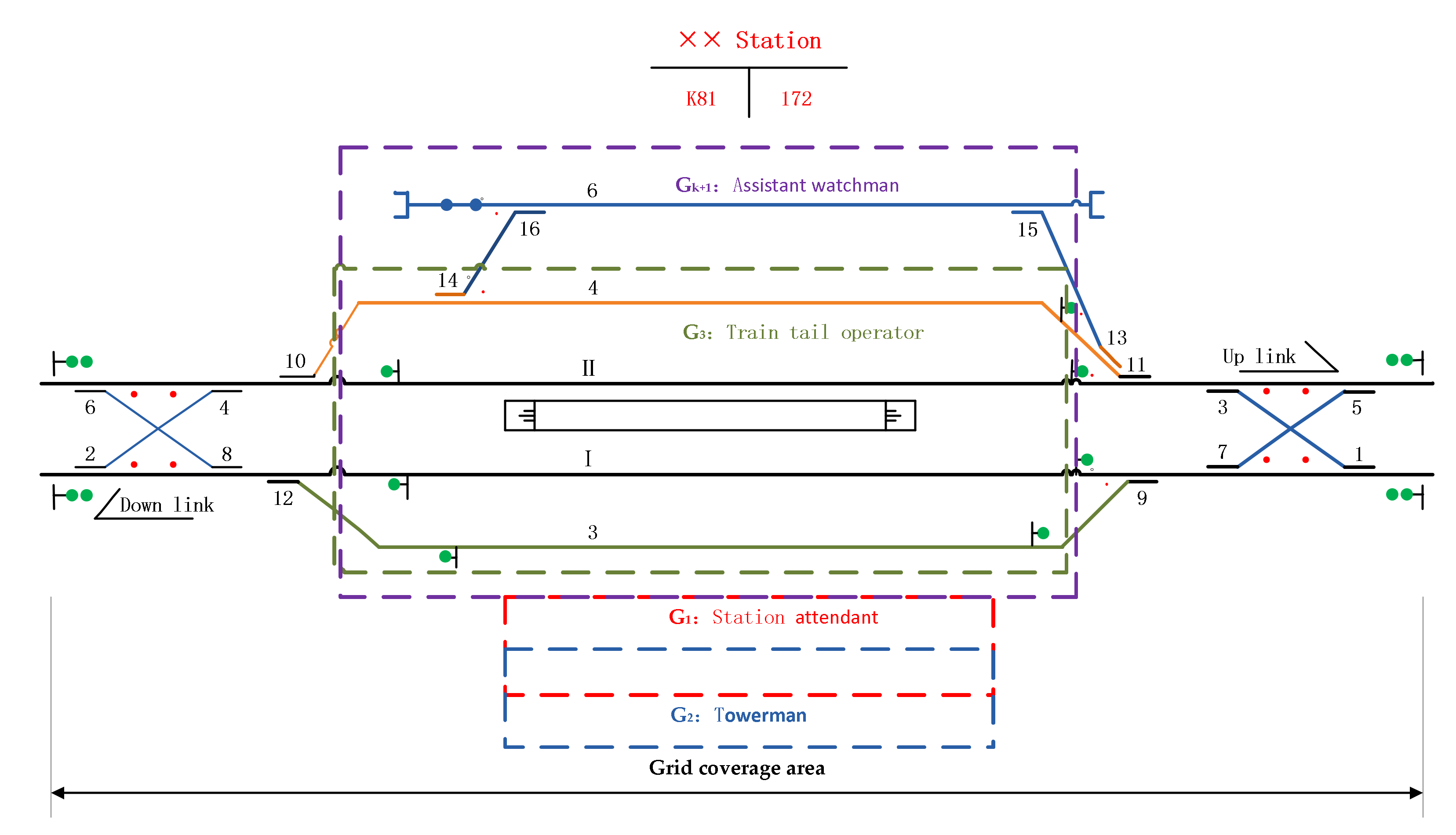
4.1. Application Scenario Description
- (1)
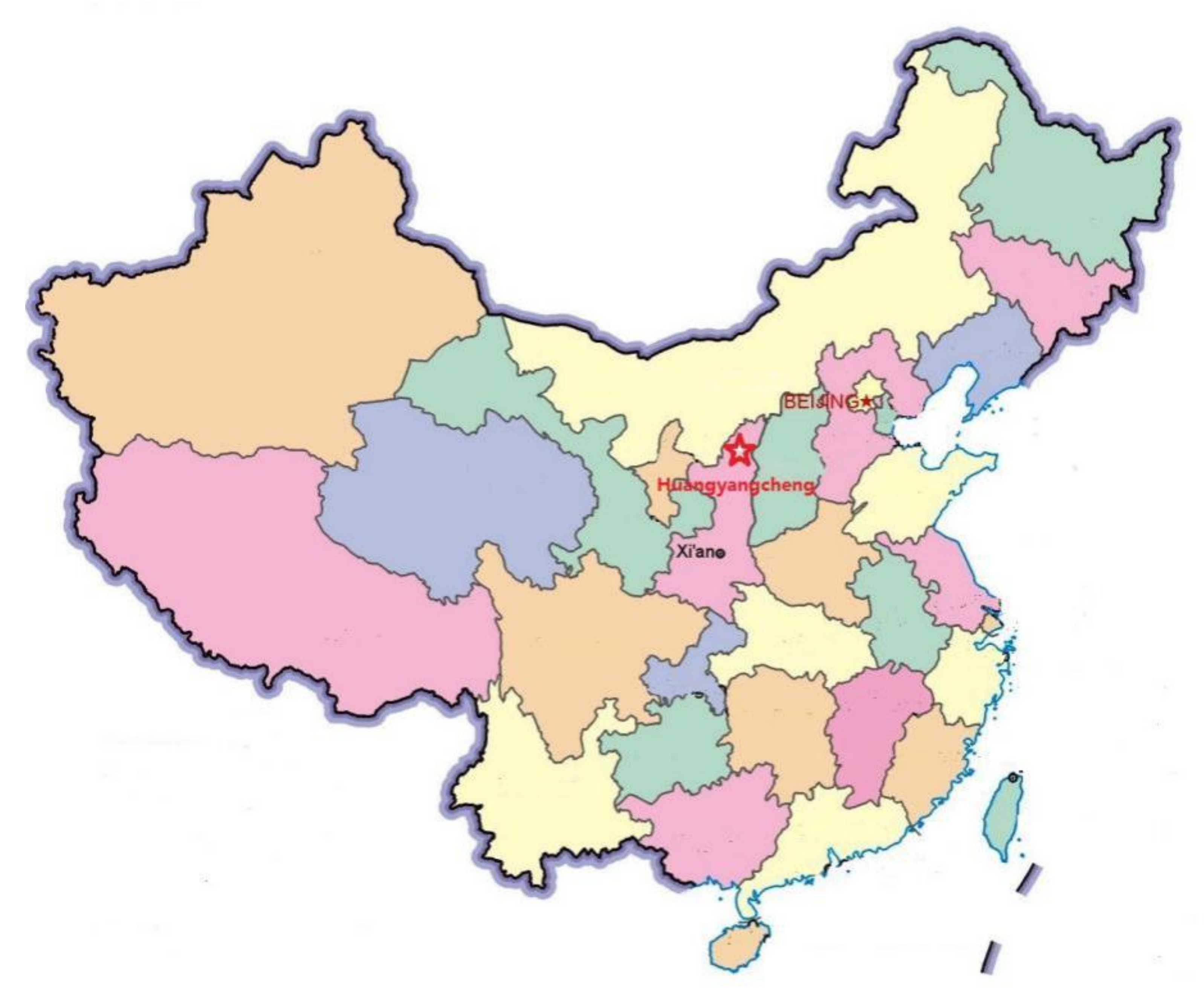
- Risk event based on data acquisition factors. Through many on-site investigations of Huangyangcheng station, we collected and sorted out a large number of hazard factor data, hidden accident dangers, and statistical accounts of education and training.
- (2)
- The operation area of the station assistant watchman spans the whole station, which has a wider operation scope than other positions and is affected by various hazard factors. If the assistant attendant does not follow the standard operation, the train operation status cannot be monitored, which may lead to derailment and personal injury. Moreover, the risk event has always been a “chronic problem” in the safety work of the station, which cannot help but be checked and prohibited, and the phenomenon of repeated occurrence is more prominent.
- (3)
- Risk event based on time characteristic factors. In view of this risk event, due to the low temperatures in winter, extremely cold weather often occurs and employees are prone to fear the cold. In addition, the inertia of station employees’ “two violations” has a certain time regularity, which is typically more in the four periods of shift handover, late midnight, lunchtime, and the weekend.
4.2. Hazard Factors Identification of “the Assistant Watchman Did Not Appear as Required”
4.3. Risk Analysis
- (1)
- Probability calculation
- (2)
- Severity calculation
- (3)
- Risk level calculation
4.4. Risk Evaluation
- (1)
- Analysis of the three-dimensional risk assessment results
- (2)
- Analysis of traditional two-dimensional risk assessment results
- (3)
- Comparative analysis
5. Conclusions
Author Contributions
Funding
Institutional Review Board Statement
Informed Consent Statement
Data Availability Statement
Acknowledgments
Conflicts of Interest
References
- Zhou, J.; Lei, Y. Paths between latent and active errors: Analysis of 407 railway accidents/incidents’ causes in China. Saf. Sci. 2018, 110, 47–58. [Google Scholar] [CrossRef]
- Zhan, Q.; Zheng, W.; Zhao, B. A hybrid human and organizational analysis method for railway accidents based on HFACS-Railway Accidents (HFACS-RAs). Saf. Sci. 2017, 91, 232–250. [Google Scholar] [CrossRef]
- Hui, X.; Yajian, Z.; Hongyang, L.; Martin, S.; Jun, Y.; Fang, Y. Safety risks in rail stations: An interactive approach. J. Rail Transp. Plan. Man 2019, 11, 100148.1–100148.11. [Google Scholar]
- ISO3100:2009; Risk Management Principles and Guidelines. ISO: Geneva, Switzerland, 2009.
- Hong, Y.; Pasman, H.J.; Quddus, N.; Mannan, M. Supporting risk management decision making by converting linguistic graded qualitative risk matrices through Interval Type-2 Fuzzy Sets. Process Saf. Environ. Prot. 2019, 134, 308–322. [Google Scholar] [CrossRef]
- Duijm, J.N. Recommendations on the use and design of risk matrices. Saf. Sci. 2015, 76, 21–31. [Google Scholar] [CrossRef] [Green Version]
- Baybutt, P. Guidelines for designing risk matrices. Process Saf. Prog. 2018, 37, 49–55. [Google Scholar] [CrossRef]
- Ghofrani, F.; He, Q.; Goverde, R.; Liu, X. Recent applications of big data analytics in railway transportation systems: A survey. Transp. Res. Part C Emerg. Technol. 2018, 90, 226–246. [Google Scholar] [CrossRef]
- Qiao, W.; Liu, Q.; Li, X.; Luo, X.; Wan, Y. Using data mining techniques to analyze the influencing factor of unsafe behaviors in Chinese underground coal mines. Resour. Policy 2018, 59, 210–216. [Google Scholar] [CrossRef]
- Dong-Han, H.; Jinkyun, P. Use of a big data analysis technique for extracting HRA data from event investigation reports based on the Safety-II concept. Reliab. Eng. Syst. Saf. 2018, 194, 106232. [Google Scholar]
- Lei, B.; Sun, Q.; Liu, R.; Wang, F.; Wang, F. A Segment-Based Model for Estimating the Service Life of Railway Rails. In Proceedings of the Cota International Conference of Transportation Professionals, Beijing, China, 25–27 July 2015. [Google Scholar]
- Liu, R.; Lei, B.; Wang, F.; Sun, Q.; Wang, F. Grid: A New Theory for High-Speed Railway Infrastructure Management. In Proceedings of the Transportation Research Board 94th Annual Meeting, Washington, DC, USA, 11–15 January 2015. [Google Scholar]
- Lei, B.; Zhang, Q.; Liu, R.; Wang, F.; Song, X. Grid-Based Framework for Railway Track Health Evaluation. In Proceedings of the International Conference on Green Intelligent Transportation System and Safety, Changchun, China, 1–2 July 2016; Springer: Singapore, 2016. [Google Scholar]
- Lei, B.; Rengkui, L.; Feng, W.; Sun, Q. Estimating railway rail service life: A rail-grid-based approach. Transp. Res. Part A Policy Pract. 2017, 105, 54–65. [Google Scholar]
- Fan, X. Research and Thinking on Grid Service and Management of Community in City S. Procedia Eng. 2017, 174, 1177–1181. [Google Scholar] [CrossRef]
- Zhang, H. A redefinition of the project risk process: Using vulnerability to open up the event-consequence link. Int. J. Proj. Manag. 2007, 25, 694–701. [Google Scholar] [CrossRef]
- Han, S.H.; Kim, D.Y.; Kim, H.; Jang, W. A web-based integrated system for international project risk management. Autom. Constr. 2008, 17, 342–356. [Google Scholar] [CrossRef]
- Duan, Y.; Zhao, J.; Chen, J.; Bai, J. A risk matrix analysis method based on potential risk influence: A case study on cryogenic liquid hydrogen filling system. Process Saf. Environ. Prot. 2016, 102, 277–287. [Google Scholar] [CrossRef]
- Meng, X.; Liu, Q.; Luo, X.; Zhou, X. Risk assessment of the unsafe behaviours of humans in fatal gas explosion accidents in China’s underground coal mines. J. Clean. Prod. 2019, 210, 970–976. [Google Scholar] [CrossRef]
- Zhang, H.; Sun, Q. Risk Assessment of Shunting Derailment Based on Coupling. Symmetry 2019, 11, 1359. [Google Scholar] [CrossRef] [Green Version]
- ISO Guide 73-2009; Risk Management Vocabulary. International Organization for Standardization, ISO: Geneva, Switzerland, 2009.
- Turner, B.L.; Kasperson, R.E.; Matson, P.A.; McCarthy, J.J.; Corell, R.W.; Christensen, L.; Eckley, N.; Kasperson, J.X.; Luers, A.; Martello, M.L.; et al. A framework for vulnerability analysis in sustainability science. Proc. Natl. Acad. Sci. USA 2003, 100, 8074–8079. [Google Scholar] [CrossRef] [Green Version]
- Sarewitz, D.; Pielke, R.; Keykhah, M. Vulnerability and Risk: Some Thoughts from a Political and Policy Perspective. Risk Anal. 2003, 23, 805–810. [Google Scholar] [CrossRef] [Green Version]
- IEC 31010-2009; Risk Management—Risk Assessment Techniques. ISO: Geneva, Switzerland, 2009.
- Huang, W.; Shuai, B.; Zhang, G. Improved WBS-RBS based identification of risks in railway transportation of dangerous goods. China Saf. Sci. J. 2018, 28, 93. [Google Scholar]
- Uğurlu, Ö.; Yıldız, S.; Loughney, S.; Wang, J. Modified human factor analysis and classification system for passenger vessel accidents (HFACS-PV). Ocean Eng. 2018, 161, 47–61. [Google Scholar] [CrossRef] [Green Version]
- Kyriakidis, M.; Majumdar, A.; Ochieng, W.Y. The human performance railway operational index—A novel approach to assess human performance for railway operations. Reliab. Eng. Syst. Saf. 2018, 170, 226–243. [Google Scholar] [CrossRef]
- Huang, W.; Shuai, B.; Zuo, B.; Xu, Y.; Antwi, E. A systematic railway dangerous goods transportation system risk analysis approach: The 24 model. J. Loss Prev. Process Ind. 2019, 61, 94–103. [Google Scholar] [CrossRef]
- GB/T 13861-2009; Classification and Code for the Hazardous and Harmful Factors in Process. General Administration of Quality Supervision, Inspection and Quarantine of the People’s Republic of China; Standardization Administration of the People’s Republic of China: Beijing, China, 2022.
- BS EN 50126-2; Railway Applications-The Specification and Demonstration of Reliability, Availability, Maintainability and Safety (RAMS)-Part 2: Guide to the Application of EN 50126-1 for Safety. British Standards Institution (BSI): London, UK, 2007.
- BS EN 50126-1; Railway Applications-The Specification and Demonstration Reliability, Availability, Maintainability and Safety (RAMS)-Part 1: Basic Requirements and Generic Process. British Standards Institution (BSI): London, UK, 1999.
- Kheybari, S.; Rezaie, F.M.; Farazmand, H. Analytic network process: An overview of applications. Appl. Math. Comput. 2020, 367, 124780. [Google Scholar] [CrossRef]
- Chukwuma, E.C.; Okonkwo, C.C.; Ojediran, J.O.; Anizoba, D.C.; Ubah, J.I.; Nwachukwu, C.P. A GIS based flood vulnerability modelling of Anambra State using an integrated IVFRN-DEMATEL-ANP model. Heliyon 2021, 7, e08048. [Google Scholar] [CrossRef] [PubMed]
- Liu, X.; Deng, Q.; Gong, G.; Zhao, X.; Li, K. Evaluating the interactions of multi-dimensional value for sustainable product-service system with grey DEMATEL-ANP approach. J. Manuf. Syst. 2021, 60, 449–458. [Google Scholar] [CrossRef]
- Salehi, R.; Asaadi, M.A.; Rahimi, M.H.; Mehrabi, A. The information technology barriers in supply chain of sugarcane in Khuzestan province, Iran: A combined ANP-DEMATEL approach. Inf. Process. Agric. 2020, 8.3, 458–468. [Google Scholar] [CrossRef]
- Nilashi, M.; Samad, S.; Manaf, A.A.; Ahmadi, H.; Rashid, T.A.; Munshi, A.; Almukadi, W.; Ibrahim, O.; Ahmed, O.H. Factors influencing medical tourism adoption in Malaysia: A DEMATEL-Fuzzy TOPSIS approach. Comput. Ind. Eng. 2019, 137, 106005. [Google Scholar] [CrossRef]
- Trivedi, A. A multi-criteria decision approach based on DEMATEL to assess determinants of shelter site selection in disaster response. Int. J. Disater Risk Reduct. 2018, 31, 722–728. [Google Scholar] [CrossRef]
- Asan, U.; Kadaifci, C.; Bozdag, E.; Soyer, A.; Serdarasan, S. A new approach to DEMATEL based on interval-valued hesitant fuzzy sets. Appl. Soft Comput. 2018, 66, 34–49. [Google Scholar] [CrossRef]
- Balsara, S.; Jain, P.K.; Ramesh, A. An integrated approach using AHP and DEMATEL for evaluating climate change mitigation strategies of the Indian cement manufacturing industry. Environ. Pollut. 2019, 252, 863–878. [Google Scholar] [CrossRef]
- Li, Y.; Mathiyazhagan, K. Application of DEMATEL approach to identify the influential indicators towards sustainable supply chain adoption in the auto components manufacturing sector. J. Clean. Prod. 2018, 172, 2931–2941. [Google Scholar] [CrossRef]
- Cagno, E.; Caron, F.; Mancini, M. A Multi-Dimensional Analysis of Major Risks in Complex Projects. Risk Manag. 2007, 9, 1–18. [Google Scholar] [CrossRef]


| Organizations, Institutions, or Scholars | Concepts |
|---|---|
| ISO [21] | The inherent nature of something that is sensitive to a risk source that can lead to a consequential event. |
| Turner [22] | The extent to which a particular system, subsystem, or component of a system may be harmed by exposure to hazards, pressures, or disturbances. |
| Sarewitz et al. [23] | A representation of the intrinsic properties of the system, which are the source of potential damage and have nothing to do with the probability of risk events occurring. |
| Main Categories | Subclass | Hazard Factors |
|---|---|---|
| Personal factors | Psychological factors | Obsessive-compulsive symptoms |
| Sensitive to interpersonal relationship | ||
| Physiological factors | somatization | |
| Professional quality | Business performance was not up to standard | |
| Low rank of professional title | ||
| Low education levels | ||
| Environment factors | Natural environment factors | Blizzard weather |
| Foggy weather | ||
| High temperature and heat | ||
| Low temperature and extreme cold | ||
| Operating environment factors | The working site conditions are inconsistent with the standards | |
| Poor lighting, ventilation, temperature, and other post conditions | ||
| Social environment factors | Poor working conditions after holidays | |
| Negative public opinion | ||
| Poor public safety environment | ||
| Equipment factors | Design and manufacturing factors | Poor equipment performance |
| Use and maintenance factors | Equipment failure | |
| Untimely maintenance | ||
| Incomplete or invalid spare parts | ||
| Management factors | Regulatory factors | Unscientific safety management system |
| Nonstandard operation standards and processes | ||
| Site management factors | The emergency operation organization is not in place | |
| Inadequate performance of safety inspection | ||
| Evaluation and supervision factors | Performance evaluation is not standardized | |
| Imperfect employment mechanism |
| Language Description | Frequency Range | Average Range | Qualitative Estimate (Number/Year) | Probability Range | Grade |
|---|---|---|---|---|---|
| Remote | 1 in 35 years to 1 in 175 years | 1 in 100 years | 0.01 | 1 | |
| Rare | 1 in 7 years to 1 in 35 years | 1 in 20 years | 0.05 | 2 | |
| Infrequent | 1 in 1.75 years to 1 in 7 years | 1 in 4 years | 0.25 | 3 | |
| Occasional | 1 in 3 months to 1 in 1.75 years | 1 in 9 months | 1.25 | 4 | |
| Regular | 1 in 20 days to 1 in 3 months | 1 in 2 months | 6.25 | 5 |
| Language Description | Qualitative Description | Casualty Estimate | Qualitative Estimate (Number/Year) |
|---|---|---|---|
| Minor | Minor injury | 0.005 | 1 |
| Marginal | Multiple minor injuries | 0.025 | 2 |
| Moderate | Single serious injury | 0.125 | 3 |
| Severe | Multiple serious injuries or single fatal injury | 0.625 | 4 |
| Catastrophic | Two to five fatal injuries | 3.125 | 5 |
| Language Description | Description | Value of Number Scale | Scale Value |
|---|---|---|---|
| Teeny | Weak feedback to the coupling effect | [1.00, 1.10) | 1 |
| Small | Slight feedback to the coupling effect | [1.11, 1.20) | 2 |
| Medium | Little reaction to the coupling effect | [1.21, 1.30) | 3 |
| Big | Obvious response to the coupling effect | [1.31, 1.50) | 4 |
| Large | Strong reaction to the coupling effect | [1.51, 2.00) | 5 |
| Risk Scores | Risk Category | Color | Description |
|---|---|---|---|
| [3, 6] | Negligible | Green | Risk is acceptable with/without the agreement of the railway authority |
| [7, 9] | Tolerable | Yellow | Acceptable with adequate control and with the agreement of the railway authority |
| [10, 12] | Undesirable | Orange | Shall only be accepted when risk reduction is impracticable and with the agreement of the railway authority |
| [13, 15] | Intolerable | Red | Risk must be reduced in exceptional circumstances |
| Main Categories | Hazard Factors |
|---|---|
| Personal factors | Obsessive-compulsive symptoms |
| Somatization | |
| Business performance was not up to standard | |
| Environment factors | Low temperature and extreme cold |
| Poor lighting, ventilation, temperature, and other post conditions | |
| Equipment factors | Equipment failure |
| Management factors | Unscientific safety management system |
| Inadequate performance of safety inspection |
| Hazards | Functions | Data | Induced Intensity | Data Sources |
|---|---|---|---|---|
| Obsessive symptom, | Symptom Check List-90 (SCL-90) test n = 2.5 | 0.006 | Shenshuo Railway “SCL-90 Mental Health Self-assessment scale” survey data, staff physical examination reports | |
| Somatization, | Symptom Check List-90 (SCL-90) test n = 1.6 | 0.003 | Shenshuo Railway “SCL-90 Mental Health Self-assessment scale” survey data, staff physical examination reports | |
| Business performance was not up to standard, | Monthly safety production knowledge test score of 85 | 0.0015 | Monthly safety production knowledge examination result of Shenshuo Railway. The examination score of 80 was qualified. | |
| Low temperature and extreme cold, | The lowest temperature of the day was −24 °C. | 0.01 | Meteorological statistics for Shenmu City | |
| Poor lighting, ventila-tion, temperature, and other post conditions, | Poor lighting conditions in the station at night | 0.003 | Daily safety inspection data and hidden trouble investigation data of Shenshuo Railway | |
| Equipment failure, | The battery capacity was insufficient, which affected the intercom call reliability | 0.004 | Equipment maintenance register | |
| Unscientific safety management system, | No mobile phone management system | 0.003 | Shenshuo railway quarterly acceptance inspection data statistics, safety audit | |
| Inadequate performance of safety inspection, | Inspection was done twice during the working week | 0.02 | Shenshuo railway quarterly acceptance inspection data statistics, safety audit |
| Hazards | Normalized by Cluster | Limiting |
|---|---|---|
| Obsessive-compulsive symptom | 0.37 | 0.19 |
| Somatization | 0.22 | 0.12 |
| Business performance was not up to standard | 0.41 | 0.21 |
| Low temperature and extreme cold | 0.61 | 0.10 |
| Poor lighting, ventilation, temperature, and other post conditions | 0.39 | 0.06 |
| Equipment failure | 0.20 | 0.06 |
| Unscientific safety management system | 0.33 | 0.11 |
| Inadequate performance of safety inspection | 0.47 | 0.15 |
| Hazard Factors | ||||||||
|---|---|---|---|---|---|---|---|---|
| 0 | 2 | 2 | 0 | 1 | 0 | 0 | 0 | |
| 1 | 0 | 2 | 0 | 0 | 0 | 0 | 2 | |
| 2 | 1 | 0 | 0 | 0 | 0 | 1 | 2 | |
| 3 | 4 | 1 | 0 | 1 | 1 | 0 | 2 | |
| 2 | 3 | 0 | 0 | 0 | 1 | 0 | 1 | |
| 0 | 1 | 0 | 0 | 1 | 0 | 0 | 0 | |
| 3 | 2 | 1 | 0 | 0 | 1 | 0 | 2 | |
| 4 | 1 | 2 | 0 | 0 | 1 | 0 | 0 |
| Row Sum | Column Sum | Coupling Strength |
|---|---|---|
| 0.55 | 1.56 | 1.39 |
| 0.57 | 1.39 | 1.36 |
| 0.68 | 1.06 | 1.32 |
| 1.28 | 0 | 0 |
| 0.72 | 0.33 | 1.19 |
| 0.22 | 0.36 | 1.10 |
| 0.96 | 0.14 | 1.19 |
| 0.82 | 0.97 | 1.33 |
| Grid Coding | Risk Size | Risk Level |
|---|---|---|
| 00010044010003020201 | 10 | Undesirable |
| 00010044010003030201 | 11 | Undesirable |
| 00010044010003040201 | 8 | Tolerable |
| 00010044010003050201 | 7 | Tolerable |
| 00010044010003060201 | 6 | Negligible |
| 00010044010003070201 | 7 | Tolerable |
| 00010044010003080201 | 9 | Tolerable |
| 00010044010003090201 | 10 | Undesirable |
| 00010044010003100201 | 8 | Tolerable |
| Risk Scores | Risk Category | Description |
|---|---|---|
| [1, 6] | Negligible | Risk is acceptable with/without the agreement of the railway authority |
| [7, 12] | Tolerable | Acceptable with adequate control and with the agreement of the railway authority |
| [13, 18] | Undesirable | Shall only be accepted when riskreduction is impracticable and with the agreement of the railway authority |
| [19, 25] | Intolerable | Risk must be reduced in exceptional circumstances |
| Date | Time | Three Violations Description | Inspection Situation |
|---|---|---|---|
| 9 January 2020 | 4:30 | Sleeping on duty | Yellow notice |
| 20 February 2020 | 23:10 | Trains were not received in time | White notice |
| 15 March 2020 | 17:00 | The busy board was not filled in timely | White notice |
| 3 April 2020 | 15:00 | Failed to use the intercom to answer the call in time | White notice |
| 17 May 2020 | 13:00 | The busy board was not filled | Yellow notice |
| 9 July 2020 | 4:30 | Dozed off on duty | White notice |
| 22 August 2020 | 7:20 | Trains were not received in time | White notice |
| 9 September 2020 | 2:30 | Sleeping on duty | Yellow notice |
| 21 October 2020 | 10:15 | Failed to use the intercom to answer the call in time | White notice |
| 5 November 2020 | 13:30 | Dozed off on duty | White notice |
Publisher’s Note: MDPI stays neutral with regard to jurisdictional claims in published maps and institutional affiliations. |
© 2022 by the authors. Licensee MDPI, Basel, Switzerland. This article is an open access article distributed under the terms and conditions of the Creative Commons Attribution (CC BY) license (https://creativecommons.org/licenses/by/4.0/).
Share and Cite
Zhang, H.; Qi, C.; Ma, M. Improved Employee Safety Behavior Risk Assessment of the Train Operation Department Based on Grids. Processes 2022, 10, 1162. https://doi.org/10.3390/pr10061162
Zhang H, Qi C, Ma M. Improved Employee Safety Behavior Risk Assessment of the Train Operation Department Based on Grids. Processes. 2022; 10(6):1162. https://doi.org/10.3390/pr10061162
Chicago/Turabian StyleZhang, Huafeng, Changmao Qi, and Mingyuan Ma. 2022. "Improved Employee Safety Behavior Risk Assessment of the Train Operation Department Based on Grids" Processes 10, no. 6: 1162. https://doi.org/10.3390/pr10061162
APA StyleZhang, H., Qi, C., & Ma, M. (2022). Improved Employee Safety Behavior Risk Assessment of the Train Operation Department Based on Grids. Processes, 10(6), 1162. https://doi.org/10.3390/pr10061162