The Role of Diffusivity in Oil and Gas Industries: Fundamentals, Measurement, and Correlative Techniques

Abstract

The existence of various native or nonnative species/fluids, along with having more than one phase in the subsurface and within the integrated production and injection systems, generates unique challenges as the pressure, temperature, composition and time (P-T-z and t) domains exhibit multi-scale characteristics. In such systems, fluid/component mixing, whether for natural reasons or man-made reasons, is one of the most complex aspects of the behavior of the system, as inherent compositions are partially or all due to these phenomena. Any time a gradient is introduced, these systems try to converge thermodynamically to an equilibrium state while being in the disequilibrium state at scale during the transitional process. These disequilibrium states create diffusive gradients, which, in the absence of flow, control the mixing processes leading to equilibrium at a certain time scale, which could also be a function of various time and length scales associated with the system. Therefore, it is crucial to understand these aspects, especially when technologies that need or utilize these concepts are under development. For example, as the technology of gas-injection-based enhanced oil recovery, CO₂ sequestration and flooding have been developed, deployed and applied to several reservoirs/aquifers worldwide, performing research on mass-transfer mechanisms between gas, oil and aqueous phases became more important, especially in terms of optimal design considerations. It is well-known that in absence of direct frontal contact and convective mixing, diffusive mixing is one of most dominant mass-transfer mechanisms, which has an impact on the effectiveness of the oil recovery and gas injection processes. Therefore, in this work, we review the fundamentals of diffusive mixing processes in general terms and summarize the theoretical, experimental and empirical studies to estimate the diffusion coefficients at high pressure—temperature conditions at various time and length scales relevant to reservoir-fluid systems.

1. Introduction

Molecular diffusion is one of the core transport mechanisms and has been of research interest to many scientists and engineers from various disciplines, including chemical reaction engineering [1,2,3,4,5], chromatography [6,7,8], separation technology [9,10,11,12], combustion technology [13,14,15,16], automotive industries [17,18,19], petroleum engineering [20,21,22,23,24,25,26,27,28,29,30], polymer science [31,32,33,34,35], biology [36,37], food technologies [38,39,40] and many more. In these applications, whenever convective mixing is not dominant, or direct frontal contact/convective mixing are absent, molecular diffusion is the only means of mixing. In addition, in many flow applications, the mixing in transverse direction (perpendicular to the flow) is governed by or coupled with molecular diffusion. For example, in porous catalysts or chemical reactors, the reactant species reach to the reacting sites via diffusion [1,2,3,4]. Similarly, diffusion-based separation is a well-known method to separate one component from the rest through molecular sieving [9,10,11,12]. Hydrogen separation from product gas streams is an example [9,41,42] of such an application. Another popular example is the separation of ortho- and para-xylene isomers where selective transport is governed by the difference in structure and hence diffusive capability through a porous medium [43,44,45].

In particular to petroleum engineering applications, diffusive mixing can be a dominant mechanism in various processes such as enhanced oil recovery in CO₂ flooding [20,21,22,23,24], Vapex [25,26], gas re-dissolution process in a depleted reservoir or solution gas drive process [27], drilling [28] and acid fracturing [29,30]. For example, in a depleted reservoir, where gas is injected to repressurize the reservoir via gas re-dissolution processes, the rate of gas dissolution is governed by molecular diffusion in the far field (because there is no mechanical/convective mixing mechanism in place within the reservoir). Thus, while the extent of dissolution (and hence re-pressurization) depends on gas solubility in the oil, the time of dissolution (or re-pressurization) is controlled mainly by molecular diffusion, even for light hydrocarbon systems [46,47,48,49,50]. In CO₂ flooding of a fractured reservoir [20,21,22,23,24], the direct contact between residual oil and CO₂ is blocked by high water saturation behind the displacement front, which prevents the development of miscibility and potentially leads to poor oil recovery. However, diffusion of CO₂ through the blocking water helps break the water barrier to a certain degree. This enables the mixing of CO₂ with residual oil, resulting in its swelling and viscosity reduction, which leads to higher oil recovery [23,24,25,26,27,28,29,30,51]. In the Vapex process for heavy oil and bitumen recovery [25,26], light hydrocarbons or non-hydrocarbons are injected. It is their diffusion into the oil beyond the potential fronts and/or convective zones that promote the effectiveness of the displacement process via reduction of in situ viscosities. In solution gas drive processes [27], the gas bubbles are evolved when reservoir pressure reduces below bubble point. It is the diffusion of gas bubbles into the oil that governs the rate of bubble growth, which directly impacts the gas mobilization and hence the oil recovery. Thus, the gas diffusivity in oil plays a key role in these displacement processes and accurate determination of it is essential to the design and understanding of such processes. In addition, the diffusive mixing is important in drilling operations [28] as well. Drilling fluids are used to insure enough hydrostatic pressure on formation to prevent the influx of formation fluids into the wellbore. However, diffusion of gases (present in the formation fluid) into the drilling fluid can lead to such an influx (also called gas kick), especially because of failures in the operation, such as insufficient drilling fluid weight and circulation loss. To detect and avoid such a mixing of gases from the formation with the drilling fluid, it is important to characterize the diffusive interactions between formation and drilling fluids along with their thermodynamic behavior.

Due to the significance of molecular diffusion in various disciplines, several studies have been performed to determine the diffusion of gas into solids and fluids. In most literature, the diffusive interactions to calculate the fluxes for the transport of molecules in oil/gases in straight tubes/pipes/pores or in the porous matrix of the catalysts/reservoir formation are characterized by the well-known Fick’s law [1]:

$$J=-D_m\nabla C$$

(1)

where $J$ is the diffusive molar flux (i.e., number of moles per unit area per unit time with the unit of ${\mathrm{mol} \mathrm{m}}^{-2}{\mathrm{s}}^{-1}$), $D_m$ is the molecular diffusion or diffusion coefficient or diffusivity (with the unit of ${\mathrm{m}}^2{\mathrm{s}}^{-1}$) and $\nabla C$ is the driving force or spatial gradient of concentration $C$. At room temperature, the typical value of diffusivity of a gas is of the order of ${10}^{-5} {\mathrm{m}}^2{\mathrm{s}}^{-1}$ into another gas, while of the order of ${10}^{-9} {\mathrm{m}}^2{\mathrm{s}}^{-1}$ in liquids and ${10}^{-12} {\mathrm{m}}^2{\mathrm{s}}^{-1}$ in solids. In dilute aqueous solutions at room temperature, the typical values of diffusion coefficients of most ions are similar to that of gas in liquids, i.e., in the range of $0.5\times {10}^{-9} {\mathrm{m}}^2{\mathrm{s}}^{-1}$ to $2\times {10}^{-9} {\mathrm{m}}^2{\mathrm{s}}^{-1}$. For biological molecules, the diffusion coefficients normally range from ${10}^{-11} {\mathrm{m}}^2{\mathrm{s}}^{-1}$ to ${10}^{-10} {\mathrm{m}}^2{\mathrm{s}}^{-1}$. While various correlations are available to estimate the diffusion of a gas into fluids/solids, very few theoretical and experimental studies are available in literature that address the diffusion of a gas in oils for the application of oil recovery, gas storage and CO₂ injection processes. Most of the theoretical studies [52,53,54,55,56,57,58] lead to correlations for diffusivity based on the well-known Stokes–Einstein relation [59] given by:

$$D_m=\frac{k_{B}T}{6\pi \mu \sigma }$$

(2)

where $T$ is temperature, $k_B$ is Boltzmann’s constant, $\mu$ is the oil viscosity and $\sigma$ is the molecular size (radius) of the gas. Note from the Stokes–Einstein relation given in Equation (2) that the gas diffusivity in a given liquid may increase with the temperature via two factors: (i) kinetic energy of the molecules ($k_{B}T$) increases with temperature leading to faster mixing and (ii) decrease in viscosity with temperature allowing better mixing. However, the increase in gas diffusivity from ambient to reservoir temperature may only be by a factor of two to three. On the other hand, the gas diffusivity can reduce significantly (i.e., several orders of magnitude) for highly viscous heavy oils as compared to that in water.

While the prediction of gas diffusivity from the Stokes–Einstein relation and similar correlations are acceptable for most gas–liquid systems containing few hydrocarbons or liquid alkanes oils, such predictions may only be qualitatively accurate for realistic gas–oil systems, especially for heavy oils and at high pressure conditions. Therefore, gas diffusivity for real oils and at reservoir conditions are obtained from experimental measurements. However, such experimental studies are limited in literature and the measurement methodologies can be classified into mainly two categories: (i) conventional and (ii) unconventional techniques. In conventional methods, direct measurement is performed for the amount of gas absorbed in the oil and spatial gradient of gas concentration in oil, which leads to the diffusivity estimation [60,61]. Such measurements require subsequent sampling and hence are system-intrusive and time consuming. On the other hand, in nonconventional techniques, a proxy measurement is performed instead of compositional measurements. The proxy quantity is then related to the diffusivity through a mathematical model that leads to estimation of the diffusivity. Examples of such indirect measurements are: (i) pressure-decay (PD) [46,47,48,49,50,52,53,56,60,61,62,63,64,65,66,67,68], (ii) constant pressure dissolving gas volumes (CPDGV) [56,60,61,62,63,64,65,66,67,68,69], (iii) the low-field nuclear magnetic resonance (NMR) [70,71], (iv) the X-ray computed assisted tomography (CAT) [72], (v) the gas permeation through immobilized liquid membrane (ILM) [73] and (vi) the dynamic pendant drop volume analysis (DPDVA) [74] methods. While each method has its own advantages and disadvantages, the PD method is the most widely used out of all these methods because of its simplicity, accuracy and convenience (while the classical methodologies may be time consuming). Therefore, we will provide a detailed review of the PD methods in a later section.

It should also be emphasized that most literature studies on experimental determination of gas diffusivity in oils deal mainly with the heavy oils or bitumens. These oils are usually in dead or near-dead conditions, i.e., have zero or very low gas-to-oil ratios (GOR). The GOR is a measure of the amount of gas dissolved in the oil and is defined as the ratio of volume of gas at standard condition (60F and 14.696 psi) liberated per unit of standard barrels of oil (when the oil is brought from reservoir conditions to the standard conditions). On the other hand, the in situ reservoir fluid systems may be in live conditions, i.e., having significant GOR. In addition, during recovery processes such as gas injection, the amount of gas dissolved in the oil may vary spatially in the reservoir, especially within the mixing zone. Since viscosity and other fluid properties depend strongly on GOR [75], the gas diffusivity may vary significantly in these mixing zones because of the GOR variation. However, there are practically no systematic experimental studies available in literature to capture the effect of the GOR on diffusivity. More recently, Ratnakar et al. [50] filled such a gap and presented the experimental data on the effect of the GOR on gas diffusivity (in oil), along with the physical interpretation of the developed empirical correlation.

In this article, we review all these aspects along with various ways to estimate the gas diffusivity. Specifically, we focus only on the calculations of molecular diffusion in all those applications that utilize conservation equations in a continuum regime (including flow simulations at various scales—micro, meso, macro or system). It should be noted that in an upscaled transport model, the effective/apparent diffusivities are utilized that depend on molecular diffusion and the coupling at scales and with other processes [4,18,30,50,76,77,78,79,80]. The estimation of the molecular diffusion part remains the same and is the focus of this work, but the coupling requires discussion case by case (i.e., coupling with flow, reaction, geometry or phases), which is out of the scope of this manuscript. In addition, calculations of diffusivities for molecular simulation may require additional efforts. Such efforts in a context of fluid-phase behavior and connection to continuum- and macro-scales can be found in the literature [81,82,83]. Therefore, this article is organized as follows: we first present the fundamental aspects of diffusion and discuss various correlations to estimate the diffusion of gas in solids, liquids and gases. Then, we review various measurement techniques to measure the diffusivity of gas in liquids and discuss one of the key measurement techniques (the pressure-decay technique) in detail. At the end, we discuss and summarize our main findings.

2. Fundamental Aspects

The concept of diffusion is usually introduced in two ways. One is the “phenomenological approach” where diffusive flux is expressed to be proportional to a driving force with the proportionality constant being a measure (or indicative) of the diffusion coefficient. Fick’s law given in Equation (1) is one of the “phenomenological approach” examples, where the driving force is the concentration gradient and the direction of the diffusive flux is from the high-concentration to the low-concentration region. Another is the “atomistic approach”, where random walk (or Brownian motion) of diffusing particles is considered. In this approach, diffusion is related to the spreading out of the particle from a point or location [59,84]. While the former approach is useful to obtain the rate of transport and identify various diffusion mechanisms, the latter approach is useful to estimate the diffusion coefficient based on intermolecular interactions or interaction of molecules with the medium. In this section, we cover the fundamental aspects of these approaches briefly.

2.1. Phenomenological Approach: Driving Force and Non-Equilibrium Thermodynamics

As stated earlier, in the phenomenological approach, diffusive flux is expressed in terms of a driving force. When the diffusion process is driven by the concentration difference, it is called ordinary or concentration diffusion. While concentration difference is normally the driving force for diffusive flux in most cases, other forces (such as pressure or temperature gradients, electrical potential, etc.) may also contribute to diffusive fluxes. In such cases, diffusion may occur from the low-concentration to the high-concentration region (intuitively contradictory to the normal diffusion). When various species diffuse under the influence of external forces, it is referred to as forced diffusion. For example, in ionic exchange membranes [85,86,87] or in charged hydrated biological tissues [88], ionic species can go under forced diffusion when exposed to an electric field. Similarly, it is called pressure diffusion when diffusive flux is caused by a pressure gradient. Microfluidic ultracentrifuge is an application example where a sufficiently large pressure gradient is applied to separate enzymes and proteins. Likewise, when diffusive flux is caused by a temperature gradient, it is called thermal diffusion or the Soret effect [89,90,91,92,93]. An important application of this effect/phenomena is the use of a Clusius–Dickel column in separation [94,95,96,97].

In addition to these driving forces, the diffusive flux of one species can also be influenced by the concentration gradient of other species in a multicomponent system, where fluxes and concentration gradients of all the species are coupled and expressed using Maxwell–Stefan equations [1,98,99]. The contribution of these driving force can be quantitatively explained using nonequilibrium thermodynamics, which is summarized in [1]. Therefore, we review some of the aspects of it here only briefly and discuss the main concept: diffusivity.

Nonequilibrium Thermodynamics and Multicomponent Diffusion

All dynamical systems that are continuously or discontinuously changing with time cannot be explained by equilibrium thermodynamics. Most of the natural systems and processes come under this category where transport and reaction are changing the behavior of such systems continuously. The behavior of such a system requires nonequilibrium thermodynamics.

While detailed concepts of nonequilibrium thermodynamics can be found in various textbooks, for example, the textbook by de Groot et al. [100], here we discuss only key points that are used to determine the driving force and the relevant model for multicomponent diffusion. The key points are as follows:

(1)

Quasi-equilibrium postulate: while real systems may lie very far from the equilibrium, especially when the gradients (in pressure, temperature, concentration, etc.) present in the system are very strong, these systems could be assumed to be in quasi-equilibrium locally, where equilibrium thermodynamics could still be applicable. Since nonequilibrium thermodynamics is still a developing area, this assumption enables us to use the equilibrium thermodynamics equations for relating state variables (especially the first and the second law of thermodynamics) as expressed by:

$$d{U}_t=Td{S}_t-Pd{V}_t+{\displaystyle \sum }_{i=1}^{N_c}{\widehat{\mu }}_{i}d{n}_i$$

(3)

where $U_t$, $S_t$ and $V_t$ are total internal energy, entropy and volume of the system, respectively; P and T are pressure and temperature, respectively; ${\widehat{\mu }}_i$ is the chemical potential of its component, $n_i$ is the number of moles of ith component; and $N_c$ is the number of components present in the system. While, in reality, the change in internal energy of the system (left-hand side of Equation (3)) is either less than or equal to the right-hand side term, locally, they are assumed to be the same.

(2)

Linearity postulate: all the fluxes in the system may be expressed as a linear combination of all the forces present in the system. This is a very important assumption that suggests that all the fluxes, such as heat flux, mass flux, momentum flux, etc., can be written as a linear function of all the driving forces, including temperature gradient ($\nabla T$), concentration or activity gradients ($\nabla c_i$ or $\nabla a_i$) of each component, pressure gradient ($\nabla P$), velocity gradient ($\nabla v$) and external forces such as gravity. This is a very important postulate that also indicates that the driving force for diffusion of species could also include the concentration/activity gradient of other species.

(3)

Curie postulate [101]: when the flux and driving forces have tensorial orders that differ by an odd number, then they are not coupled with each other. Note that the heat and mass transfer fluxes are vectors (tensor of order unity) while the gradient in velocity ($\nabla v$) is a second order-tensor. Thus, the deference in their tensorial order is unity (an odd number) and, hence, according to the Curie postulate, the heat and mass transfer fluxes cannot depend on velocity gradient directly. In other words, heat and mass transfer fluxes depend directly only on concentration/activity gradients, pressure gradients, temperature gradients and external forces. Indirectly, these fluxes can depend on the velocity gradient only when it creates gradients in concertation, temperature and/or pressure.

(4)

Symmetry (Onsager’s reciprocal approximation [102,103]): the coefficient matrix relating the flux and driving force is symmetric. This leads to the diffusivity and conductivity matrices being symmetric. (Note: it was shown later by Truesdell [104] using second law of thermodynamics that the diffusivity and conductivity tensors must be positive definite.)

The above postulates coupled with mass, momentum and energy conservations laws lead to the multicomponent diffusion model as follows (see the detail in [1,100,105,106,107,108,109]):

$$J_k=-D_k^T\nabla \ln T-{\displaystyle \sum }_{j=1}^{N_c}{D}_{kj}{x}_k\left[x_j\nabla \ln a_j+\left(\frac{x_j{\widehat{V}}_j}{RT}\right)\nabla p-\left(\frac{x_j}{RT}\right)g_j\right]$$

(4)

where $J$ is the diffusive flux; $a$ is the activity; $x$ is the mole fraction; $\widehat{V}$ is the partial molar volume; and $g$ is the external force per mole. The first term represents the thermal diffusion where $D_k^T$ is the multicomponent thermal diffusion coefficient that satisfies: $\sum _k{D}_k^T=0$. The second term represents the diffusional driving force that consists of a concentration/activity gradient, a pressure gradient and external forces (forced diffusion). Here $D_{kj}$ can be referred as the multicomponent diffusivity, which may be different than the binary diffusivities. Equation (4) is also referred to as the generalized Fick’s law.

The above four postulates and conservation laws can also be rearranged to express the diffusional flux and driving forces in more general form, as follows:

$$d_j=-{\displaystyle \sum }_{i\ne j}^{N_c}\frac{x_i{x}_j}{D_{ij}^{\prime }}\left(\frac{D_j^T}{c_j}-\frac{D_i^T}{c_i}\right)\nabla \ln T-{\displaystyle \sum }_{i\ne j}^{N_c}\frac{\left(x_i{J}_j-x_j{J}_i\right)}{c{D}_{ji}}$$

(5)

where $d_j$ is the net diffusional driving forces (including concentration/activity, pressure, and forced diffusion), expressed as follows:

$$cRT{d}_j=c_{j}RT\nabla \ln a_j+\left(c_j{\widehat{V}}_j-x_j\right)\nabla p-c_j{g}_j+x_j{\displaystyle \sum }_{i=1}^{N_c}{c}_i{g}_i$$

(6)

where $c_j$ is the molar concentration of jth component and $c$ is the total molar concentration. The above Equations (5) and (6) are referred to as generalized Maxwell–Stefan equations. Note that the diffusivities $D_{ij}$ in Equation (5) may not be the same as the diffusivities $D_{ij}$ in Equation (4).

For the case of multicomponent low-density gases, the activity coefficients can be taken as a unity, (i.e., $a_j=c_j=c{x}_j$). In this case, when the concentration gradient is the only driving force, the multicomponent diffusion model (Equations (5) and (6)) reduces to the well-known Maxwell–Stefan equation [1,98,99]:

$$\nabla x_j=-{\displaystyle \sum }_{i=1}^{N_c}\frac{\left(x_i{J}_j-x_j{J}_i\right)}{c{D}_{ji}}={\displaystyle \sum }_{i=1}^{N_c}\frac{\left(x_i{N}_j-x_j{N}_i\right)}{c{D}_{ji}}={\displaystyle \sum }_{i=1}^{N_c}\frac{x_i{x}_j\left(v_j-v_i\right)}{D_{ji}}, j=1,2,\dots N_c$$

(7)

where $D_{ji}$ is the binary diffusivity; $N_i=J_i+c{x}_i{v}^{*}$ is the net molar flux including the diffusive and convective fluxes; and $v^{*}$ is the molar velocity of the gas. As per Onsager’s reciprocal approximation, the diffusivities $D_{ji}$ are symmetric, i.e., $D_{ji}=D_{ij}$.

The Maxwell–Stefan model (Equation (7)) is also obtained by extending the Chapman–Enskog theory to a multicomponent system [110]. While this is good for low-density gases, they work well even with dense gases, liquids and polymers, with the exception that the diffusivities may be different than binary diffusivity and may be strongly dependent on concentration. It can also be seen that when there are only two components, Equation (7) reduces to the Fick’s law, given in Equation (1), where diffusion flux of a component is always proportional to the negative of its concentration gradient. However, for a multicomponent system, this may not be the case. In fact, a component can diffuse in the absence of its concentration gradient or against its own gradient, depending on other driving forces. In addition, the diffusion flux of a component may be zero (i.e., no diffusion), even when its concentration gradient is present (this is called barrier diffusion). Furthermore, the diffusion flux may not be collinear with the concentration gradient of the other species.

However, in most practical applications, diffusive flux is proportional to the negative of the concentration gradients of all concentrations and can be represented by the multicomponent version of Fick’s law as:

$$J_k={\displaystyle \sum }_{i=1}^{N_c}c{D}_{ki}\nabla x_i, k=1,2,\dots N_c$$

(8)

where $D_{ki}$ is the binary diffusivity. In the case of dilute systems, Fick’s law can be simplified further to:

$$J_k=c{D}_{km}\nabla x_k, k=1,2,\dots N_c$$

(9)

where $D_{km}$ is the diffusivity of kth component in the mixture. In the following sections, we present various correlations and experimental techniques to obtain this quantity.

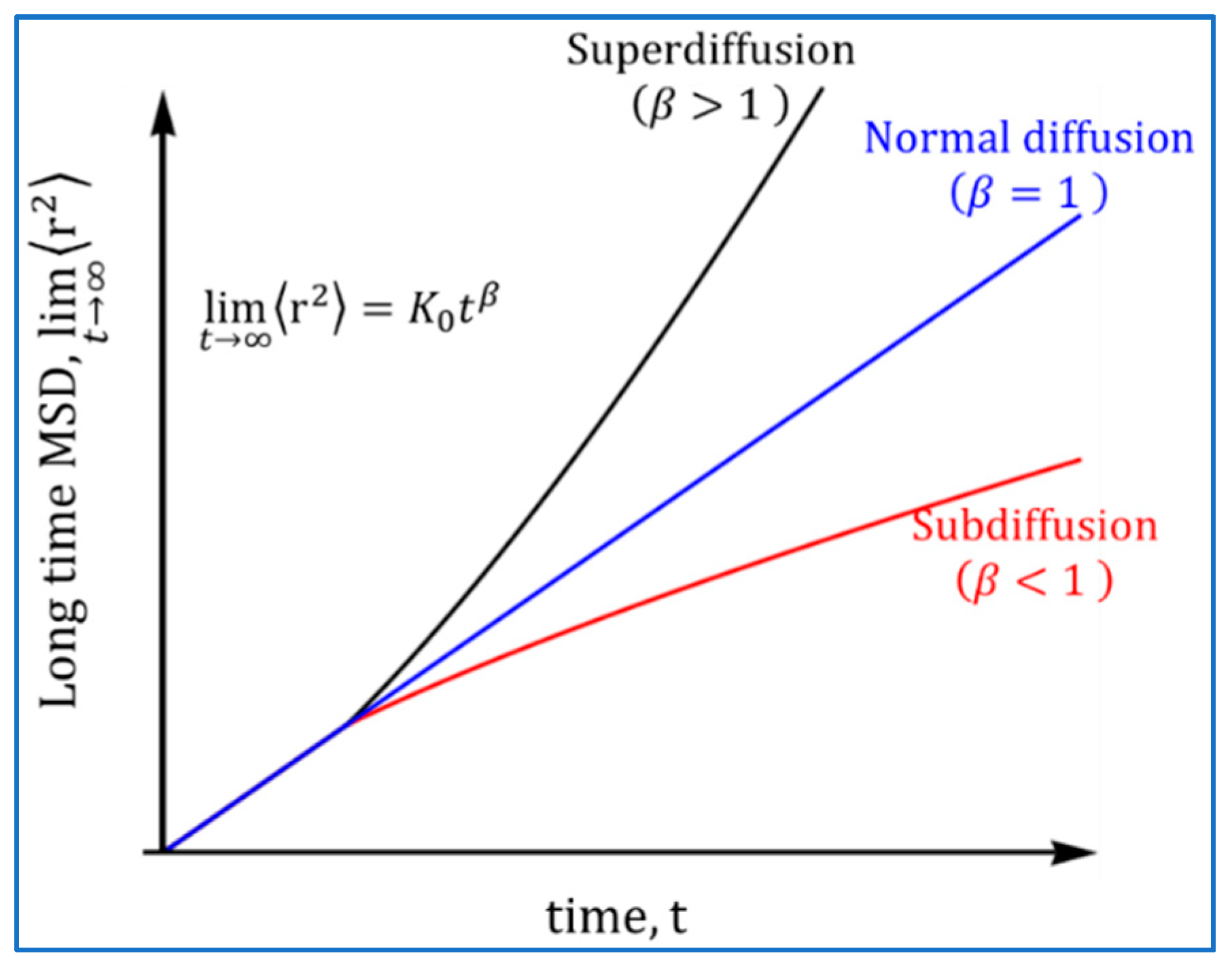
2.2. Atomistic Approach: Normal and Anomalous Diffusion

The atomistic approach is based on the modeling of Brownian motion of atomic particle by Einstein [59,84], who defined diffusion as a means of spreading out particles from a point location in an irregular/random walk motion. The notion of Brownian motion came into the picture by the experiments performed by Brown [111,112] on random trajectories of small particles of pollen and inorganic matter. This irregular motion was modeled by random walk by Einstein [59,84], where the mean square displacement of particles $\langle {\left(\mathsf{\Delta }r\right)}^2\rangle$ increases with time $t$ in linear fashion as follows:

$$\underset{t\to \infty }{\lim }\langle r^2\rangle =2s{D}_{m}t,$$

(10)

where s is the spatial dimension and $D_m$ is the diffusivity. Equation (10) was obtained by combining the kinetic theory with Fick’s law, leading to a 1D transient diffusion equation in number density $n\left(x,t\right)$ as:

$$\frac{\partial n\left(x,t\right)}{\partial t}=D_m\frac{{\partial }^{2}n\left(x,t\right)}{\partial x^2}; n\left(x\ne 0,t=0\right)=0; {{\displaystyle \int }}_{-\infty }^{\infty }n\left(x,t\right)dx=N_t,$$

(11)

which after solving (with the assumption of symmetry, i.e., $n\left(-x,t\right)=n\left(x,t\right)$ and the total $N_t$ particles located initially at the origin) gives the solution as:

$$n\left(x,t\right)=\frac{N_t}{\sqrt{4\pi D_{m}t}}\exp \left(-\frac{x^2}{4D_{m}t}\right).$$

(12)

The above solution yields the mean square displacement as:

$$\underset{t\to \infty }{\lim }\langle x^2\rangle =\frac{1}{N_t}{{\displaystyle \int }}_{-\infty }^{\infty }{x}^{2}n\left(x,t\right) dx=2D_{m}t.$$

(13)

This result can easily be generalized for 2D and 3D, which in general could be written as in the form of Equation (10). Furthermore, considering the molecules as non-interacting spherical particles with radius $r_p$ in a liquid with viscosity $\mu$, Einstein [59] developed the well-known Stokes–Einstein relation expressed by Equation (2), which forms a basis for many correlations developed in the literature [52,53,54,55,56,57,58] for estimating the diffusivity of gas in oils.

It should be noted that the linear relationship between mean square displacement and time may not always be applicable. When the relationship between the two is linear, it is called normal diffusion, otherwise called anomalous diffusion. The cause of anomalous (non-linear) behavior can vary from system to system and may include factors such as heterogeneity and complexity in the medium, fractal structure and geometries, interaction between various length and time scales, and many more. Such anomalous behavior is represented as power-law as given by:

$$\underset{t\to \infty }{\lim }\langle r^2\rangle =K_0{t}^{\beta },$$

(14)

where $K_0$ is called the generalized diffusion coefficient and the power index $\beta$ depends on the system under consideration. For example, it is called normal diffusion when $\beta =1$, subdiffusion when $\beta <1$ and superdiffusion when $\beta >1$ (see Figure 1). Since oil-and-gas-industry-related applications utilize the phenomenological description of diffusion processes (coupled with velocity gradients when flow is present) to model the transport of gases in oil reservoirs, we limit the atomistic description to only a basic introduction and refer the details to the published literature [113,114,115,116,117,118,119,120,121,122,123,124,125].

3. Physics-Based and Empirical Correlations for Diffusivity Estimation

As discussed earlier, diffusion coefficients are required for the calculation of fluxes for the transport of molecules in straight pores or in porous media including the porous matrix of the catalysts and reservoir formations. Depending on the molecular size and pore size of the capillary or the fabric of the porous matrix/tortuosity, the diffusivity of a gas varies in orders of magnitude. Figure 2 shows schematics of the order of diffusivities of gases with respect to pore size (obtained from [3,126]).

It can be seen from this figure that when the pore size is large (greater than 2000 Ǻ or 0.2 µm), regular or bulk diffusion occurs where diffusivity is roughly in the order of 1 cm²/s, while for pores with sizes between 10–2000 Ǻ the molecules are either in a transition regime or Knudsen regime where diffusivity decreases with pore size. Typically, the Knudsen diffusivity in a porous matrix is in the order of 10⁻⁴ to 1 cm²/s and depends on gases. However, under vacuum or extremely low-pressure conditions or free space, it can be as high as 104 cm²/s. In pores with sizes below 10 A°, either no diffusion takes place or configurational diffusion takes place. More detailed discussion will be presented below. Figure 2 also shows schematically that (i) the bulk diffusivity of gases may decrease with pressure and (ii) diffusivity of gases in liquids are typically of the order of 10⁻⁶ to 10⁻⁵ cm²/s, which is usually lower than the Knudsen diffusivity. In the rest of this section below, we briefly review various mechanisms of diffusion and the correlations to estimate the corresponding diffusion coefficients in gas- and liquid-filled pores in a straight capillary and in a porous material.

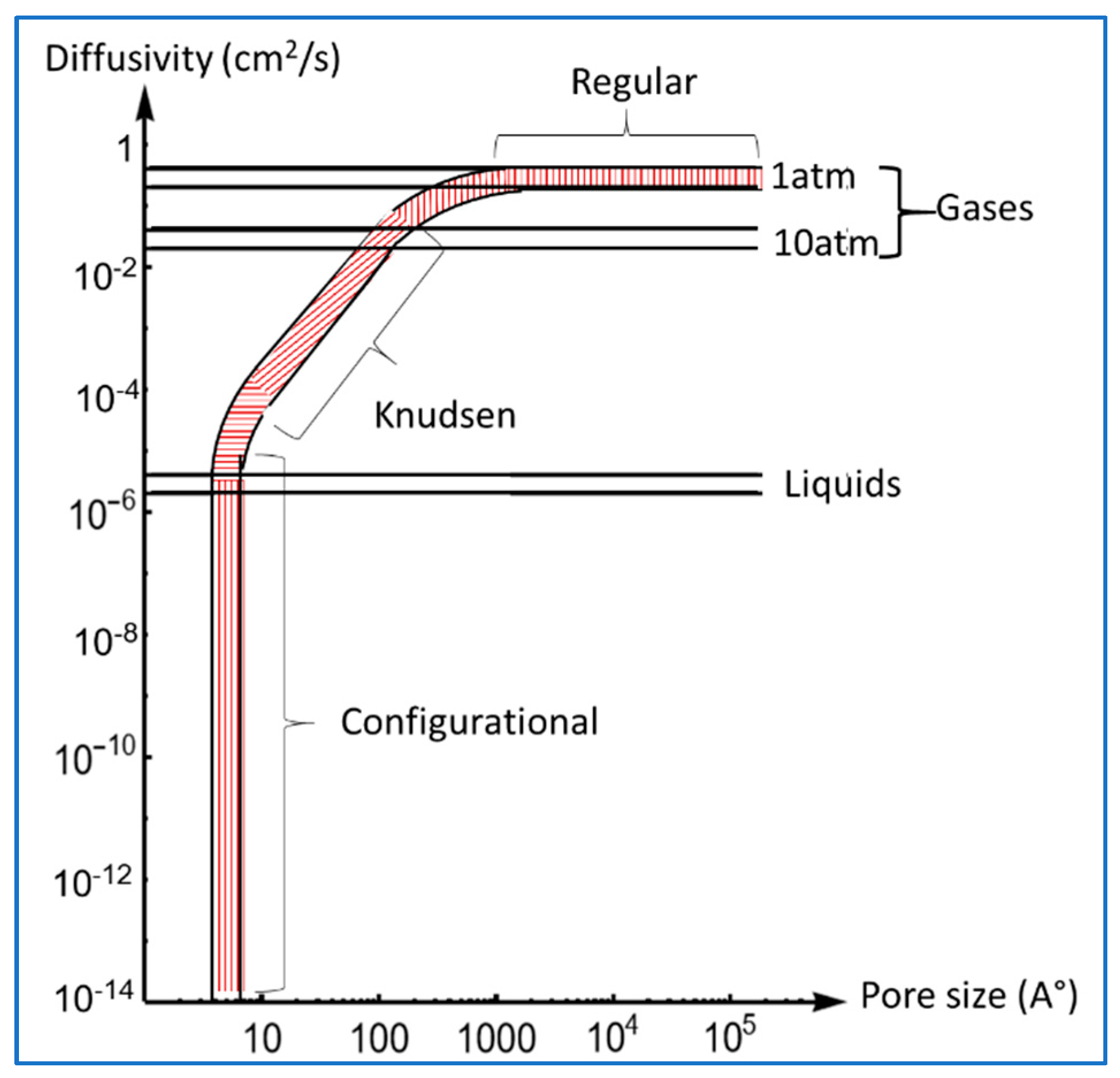
3.1. Various Mechanism of Diffusion in a Capillary

There are primarily six mechanisms for molecular transport in a capillary [3,5], namely (i) viscous flow, (ii) bulk diffusion, (iii) Knudsen diffusion, (iv) surface diffusion, (v) capillary condensation, and (vi) activated diffusion (see Figure 3 for schematics). One particular mechanism may be dominant over another depending on pressure, temperature, pore size and pore-fluid interactions. In addition, the diffusion rate may also vary from one mechanism to another. For example, a gas can diffuse faster if the pore size is larger, while diffusion can be slower or restricted when the pore size is smaller. Similarly, the chemistry at the pore level (such as adsorption) can also alter the way a gas will diffuse through the pore. In general, the diffusion rate decreases as we go from viscous flow (first mechanism) to activated diffusion (sixth mechanism). In the first two mechanisms (viscous flow and bulk diffusion), where the diffusion rate is higher, the diffusion is independent of solid–fluid interaction and the property of the fluid is the same as in the bulk (uniform), while in the other mechanisms (Knudsen, surface, capillary condensation and activated diffusion), the fluid may interact with pores and the fluid properties may be different than the properties in bulk.

The underlying causes for these transport mechanisms vary (see [3,5] for brief summary). For example, viscous flow in a large pore is governed by the pressure difference, $\mathsf{\Delta }P$, across the pore, where flow velocity of the fluid is expressed by the Hagen–Poiseuille law [1]. For dilute gas mixtures, since pressure and concentration are related by the ideal gas law, $P=cRT$, the viscous flux $N_k^v$ of a gaseous solute (kth species) can be represented as the concentration gradient ($\mathsf{\Delta }c$) over the pore length $\left(L\right)$, as follows:

$$N_k^v=c_{k}v=c_k\frac{d_p^2\left(-\mathsf{\Delta }p\right)}{32\mu L}=c_k\frac{d_p^{2}RT\left(-\mathsf{\Delta }c\right)}{32\mu L}=\left(\frac{d_p^{2}RTc}{32\mu }\right)\left(\frac{-\mathsf{\Delta }{c}_k}{L}\right),$$

(15)

This leads to the proportionality factor (or equivalent diffusivity or pressure diffusivity) expressed by $D_{visc,k}=\frac{d_p^{2}RTc}{32\mu }$, which is a function of pressure (or concentration) and temperature and the pore size $d_p$.

When the overall pressure difference is zero (i.e., $\mathsf{\Delta }p=0$), but not the partial pressure of an individual species, this leads to the concentration difference of the species across the subject pore. Such concentration differentials lead to molecular diffusion and are expressed in terms of Fick’s law as shown in Equation (1). In such cases, when a pore is large enough (as compared to the mean free path of the gas), the transport is expressed in terms of bulk diffusivity. But when pore size is small (i.e., the same order as the mean free path of the molecule), the transport is governed by the Knudsen diffusivity. Additionally, when the pore size is of the same order as (slightly larger than) the size of the molecule, the transport is referred to as molecular sieving or configurational diffusion or activated diffusion. Molecular sieving has been exploited in many separation applications such as separation of the linear alkanes from branched alkanes (including isomers). For example, para-xylene (being linear molecules) can diffuse faster in the pores of a zeolite than the branched ortho- or meta-xylene when pore size is comparable to the molecular size. In the case of external forces such as electric fields acting as potential barriers, the small-charged molecules can diffuse even faster. This is one way to sperate protons (hydrogen) and is referred to as activated diffusion.

The gaseous molecules can also interact with the solid surface and can get adsorbed physically or chemically. In the case of physisorption (i.e., when adsorption energy is less than $k_{B}T$), molecules are loosely bound with the surface and are mobile. In this case, the flux is represented as Fick’s law with the driving force being the difference in adsorbed concentration. However, in the case of chemisorption (i.e., when adsorption energy is greater than $k_{B}T$), the gas molecules are tightly bound and require additional heat to desorb. In this case, the molecules are tightly bound with the surface (with hindered mobility) and move along the surface by hopping from one site to other. This adds to the net flux of the molecules and is expressed in terms of surface diffusivity similar to Fick’s law. In both of these cases, accumulation to the surface and hopping along the surface leads to effective diffusivity being dependent on the adsorption isotherm (see [3,6,77,127]).

Finally, when pore sizes are too small (lower than the Knudsen and surface diffusion regime), the vapor pressure of gases may be altered because of the pore confinement (see the brief review in [81]). Therefore, when the temperature is below critical value (i.e., in subcritical region), phase change may occur because of altered vapor pressure and gases could condensate to form a liquid phase. This is referred to as capillary condensation. The condensation could lead to a convective flow of the gas, resulting in much faster transport as compared to diffusion alone. In this case, the effective diffusion coefficients are comprised of diffusion and convection contributions [5] (i.e., dispersion). Since the critical temperature of CO₂ is 304 K, while that of methane is 190.56 K, separation of CO₂ from methane could be performed at room temperature (~298 K), taking advantage of the capillary condensation phenomenon. Another example is cryo-pumping [128,129] to create vacuum in many applications (though cryo-pumping may also cause integrity issues in some applications such as cryogenic hydrogen storage—see the review paper [130]).

3.2. Diffusion in Gas-Filled Pores

As discussed earlier, viscous flow is driven by the overall pressure difference across a pore, while bulk and Knudsen diffusion are driven by the difference in partial pressure or concentration across the pore. Capillary condensation is important when dealing with vapor and may consist of diffusion in both gases and saturated liquids. The surface diffusion can also be significant because of adsorption, such as in unconventional reservoirs and chromatography applications. The activated or configurational diffusion may be important in separating isomers or when dealing with charged particles or when potential barrier exists. The importance of these mechanisms depends on the relative size of molecules $\sigma$ and mean free path $\lambda$ to the pore diameter $d_p$.

The mean free path $\lambda$ is the average distance traveled by the molecules between collisions, and may be obtained from the kinetic theory of gases at pressure P as:

$$\lambda =\frac{1}{\sqrt{2} \pi {\sigma }^2{n}_g }=\frac{k_{B}T}{\sqrt{2} \pi {\sigma }^{2}P},$$

(16)

where $n_g$ is the number density of the molecule (i.e., number of molecules per unit volume). The ratio of the mean free path to the pore diameter is called Knudsen number $K_n$, i.e.,:

$$K_n=\frac{\lambda }{d_p}=\frac{k_{B}T}{\sqrt{2} \pi {\sigma }^{2}P{d}_p }$$

(17)

Similarly, the mean velocity of the molecule from the kinetic theory of gases can be expressed as:

$$\overline{v}=\sqrt{\frac{8RT}{\pi M_w}} ,$$

(18)

where $M_w$ is the molecular weight of the subject gas and R is the gas constant.

In most applications, such as catalytic reactors and reservoir formations, the dominant mechanisms of molecular transport are viscous flow, bulk diffusion and Knudsen diffusion. The diffusivity corresponding to the viscous flow is described earlier in Equation (15), the Knudsen and bulk diffusivity in the next two subsections.

3.2.1. Knudsen Diffusion ($K_n\gg 1$ or $\lambda \gg d_{\mathrm{p}}$)

When Knudsen number $K_n$ is high (>> 1), i.e., mean free size is greater than the pore size, most molecules collide with the wall before they collide with each other. In this case, the molecular transport is mainly due to the collisions with the walls and is referred to as the Knudsen flow. In this case, the average distance traveled between the molecule–wall collision can be assumed to be same as pore diameter, and hence the Knudsen diffusivity, $D_{Kn},$ can be expressed as:

$$D_{Kn}=\frac{1}{3}{d}_p\overline{v}=d_p\sqrt{\frac{8RT}{9\pi M_w}}=0.532d_p\sqrt{\frac{RT}{M_w}} .$$

(19)

Equation (19) suggests that the Knudsen diffusion of a gas is independent of pressure and primarily depends on temperature, molecular weight of the gas and the pore diameter. In the case of irregular-shaped pores, the diameter can be replaced by the characteristic pore size (which is the ratio of volume to the surface area). Typical values for Knudsen diffusivity in a porous matrix are in the range of 10⁻⁴ to 1 cm²/s as shown in Figure 2. Under low-pressure (or near-vacuum) conditions, the mean free path can be very small (see Equation (17)), which may lead to a Knudsen flow regime and diffusivity can be as high as 10⁴ cm/s.

3.2.2. Bulk Diffusion ($K_n\ll 1$ or $\lambda \ll d_{\mathrm{p}}$)

When Knudsen number $K_n$ is low (<< 1), i.e., the mean free path is smaller than the pore size, most molecules collide with each other and spread in every direction (unless restricted by the pore wall). In this case, the molecular transport is mainly due to the collisions between molecules and is referred to as bulk diffusion. Thus, the bulk diffusivity is independent of the wall effects and the average distance traveled by the molecules before sequential collision is the same as the mean free path. This leads to the bulk diffusivity $D_m$ from the kinetic theory of gases as:

$$D_m=\frac{1}{3}\lambda \overline{v}=\frac{1}{3}\frac{k_{B}T}{\sqrt{2} \pi {\sigma }^{2}P }\sqrt{\frac{8RT}{9\pi M_w}}\propto \frac{T^{3/2}}{P{M}_w^{1/2}{\sigma }^2}.$$

(20)

Equation (20) suggests that the bulk diffusivity depends on the pressure (unlike the Knudsen diffusivity) and gas properties. Following the same concept as in Equation (20), the bulk diffusivity can be obtained from two ways as described below.

Chapman–Enskog formula. The binary diffusivity for a mixture of gases A and B can be obtained from the Chapman–Enskog formula as derived and described in [1,131] as follows:

$$D_{AB}=\frac{0.0018583}{P{\sigma }_{AB}^2{\mathsf{\Omega }}_{AB}}\sqrt{T^3\left(\frac{1}{M_{w,A}}+\frac{1}{M_{w,B}}\right)}; \left[D_{AB}\right]={\mathrm{cm}}^2{\mathrm{s}}^{-1};\left[P\right]=\mathrm{bar}; \left[{\sigma }_{AB}\right]={\mathrm{A}}^{°}$$

(21)

where $M_{w,A}$ and $M_{w,B}$ are the molecular weights of the gases A and B, respectively; ${\sigma }_{AB}=\frac{\left({\sigma }_A+{\sigma }_B\right)}{2}$ is the mean of molecular sizes ${\sigma }_A$ and ${\sigma }_B$ of gases A and B, respectively, which is also referred to as the characteristic length of the intermolecular force law; and ${\mathsf{\Omega }}_{AB}$ is the collision integral for diffusion for the binary gas mixture that depends on the temperature and the intermolecular interaction energies between the colliding molecules.

The collision integral ${\mathsf{\Omega }}_{AB}$ is obtained from the Lennard–Jones parameters. For example, one of the well-known correlations for expressing intermolecular energy $\psi$ in terms of intermolecular distance $r$ is given from the Lennard–Jones potential model [132,133,134]:

$$\psi =4ϵ\left[{\left(\frac{\sigma }{r}\right)}^{12}-{\left(\frac{\sigma }{r}\right)}^6\right]$$

(22)

where $ϵ$ and $\sigma$ are characteristic Lennard–Jones energy and length, respectively. For binary mixtures, these parameters are given by geometric and arithmetic mean, respectively, i.e., ${ϵ}_{AB}=\sqrt{{ϵ}_A{ϵ}_B}$ and ${\sigma }_{AB}=\frac{\left({\sigma }_A+{\sigma }_B\right)}{2}$. The collision integral ${\mathsf{\Omega }}_{AB}$ is expressed by using these parameters as a function of $\frac{k_{B}T}{{ϵ}_{AB}}$ (see [131] for various approximations). One of the accurate correlations proposed by Neufeld et al. [135] is:

$${\mathsf{\Omega }}_{AB}=\frac{1.06036}{T_D^{0.15610}}+\frac{0.19300}{\exp \left(0.47635T_D\right)}+\frac{1.03587}{\exp \left(1.52996T_D\right)}+\frac{1.76474}{\exp \left(3.89411T_D\right)};$$

(23)

where $T_D=\frac{k_{B}T}{{ϵ}_{AB}}.$

The values of energy $ϵ$ and length $\sigma$ for various gases can easily be found in the literature [131]. When these parameters are not available, following empirical expression for $T_D$ in terms of critical temperature, $T_c,$ and molar volume, ${\widehat{V}}_b,$ can be used (see [131] for details).

$$T_D=\frac{k_{B}T}{{ϵ}_{AB}}\approx \frac{1.3T}{T_c}; \sigma \approx 1.18 \sqrt[3]{{\widehat{V}}_b} ; \left[\sigma \right]={\mathrm{A}}^{°}; \left[{\widehat{V}}_b\right]={\mathrm{cm}}^3{\mathrm{mol}}^{-1}$$

(24)

Fuller–Schettler–Giddings correlation. An alternate method to estimate bulk diffusivity of a binary gas mixture is based on the Fuller–Schettler–Giddings correlation [136]:

$$D_{AB}=\frac{{10}^{-3}{T}^{1.75}}{P{\left[{\left({\sum }_A\widehat{V}\right)}^{\frac{1}{3}}+{\left({\sum }_B\widehat{V}\right)}^{\frac{1}{3}}\right]}^2}\sqrt{\left(\frac{1}{M_{w,A}}+\frac{1}{M_{w,B}}\right)}; \left[D_{AB}\right]={\mathrm{cm}}^2{\mathrm{s}}^{-1};\left[P\right]=\mathrm{bar};$$

(25)

where $\sum _A\widehat{V}$ represents the diffusion volume of gas A, which can be either obtained directly from

Table 1. Atomic diffusion volumes obtained from [131].

Atomic and Structural Diffusion Volume Increment for Various Substances
C	15.9	H	2.31	O	6.11	N	4.54
F	14.7	Cl	21.0	Br	21.9	I	29.8
S	22.9	Atomic ring or Heterocyclic ring			−18.3
Diffusion volume for simple molecules
He	2.67	Ne	5.98	Ar	16.2	Kr	24.5
Xe	32.7	H2	6.12	D2	6.84	N2	18.5
O2	16.3	CO	19.0	CO2	26.9	N2O	35.9
NH3	20.7	H2O	13.1	SF6	71.3	Cl2	38.4
Br2	69.0	SO2	41.8	Air	19.7

provided in [131,136] or by summing the diffusion volume of all atoms of A from the same table. These values (obtained from [131]) are reported here in Table 1 for the completeness.

For example, to calculate the diffusion volume of CHCl₃, Table 1 can be used to sum the diffusion volume of all atoms as: $\sum _A\widehat{V}$ = $\left(1\right) \left(15.9\right)+\left(1\right)\left(2.31\right)+\left(3\right)\left(21.0\right)=60.21$, and so forth.

Thus, when the Lennard–Jones parameters are not available for some molecules, then the Fuller–Schettler–Giddings correlation (Equation (25) can be utilized to estimate the diffusivity, and vice versa. It should be noted that this correlation suggests that the bulk diffusivity varies by the power-law of temperature with the exponent of 1.75, while the Chapman–Enskog theory (Equation (21)) suggests the exponent to be 1.5 when the collision integral has weak dependence on temperature. The error in estimation from both methods is small (within 2%) for most typical gases at ambient (or close to ambient) conditions. The typical range of bulk diffusivity is in the range of 0.1 to 1 cm²/s as shown in Figure 2

3.3. Diffusion of Gases in Porous Media

Porous media such as a porous catalyst or reservoir formation have complicated irregular and interconnected pores, which alters the diffusivity, as presented earlier for a single straight pore. To describe the molecular diffusion flux in porous media, the two main factors must be accounted for: (i) only a fraction of the porous media is available for molecules to move—an effect of porosity, and (ii) pores are irregular, interconnected and tortuous—effects of tortuosity and connectivity.

The most simplified modification is obtained by considering the effective gradient length being increased because of tortuosity (one of the measures of the distance traveled, which is also related to system permeability) and is given by:

$$D^e=\frac{D_m\epsilon }{\tau },$$

(26)

where $\epsilon$ and $\tau$ are the porosity and tortuosity of the porous media; and $D^e$ is the effective diffusivity. While this approximation is good for narrow pore size distribution, it may not lead to accurate estimation for wide pore distribution where the range of pore size are significant (i.e., varying from continuum to Knudsen or configurational regime). For example, when pore sizes are close to the mean free path of the molecule, the approximation given in Equation (26) may be appropriate with $D_m$ being the Knudsen diffusivity $D_{Kn}.$ Similarly, when the majority of the pores are larger than the mean free path of the molecules, the approximation given in Equation (26), with $D_m$ being the bulk diffusivity, may be acceptable. However, when pore sizes include both of these regimes, the effective diffusivity in the porous media must contain all diffusional resistances.

Figure 2 shows the typical ranges of pore size for the Knudsen and continuum regimes. When pore size distribution is such that both Knudsen and bulk diffusion transport may be dominant, depending on the pore size and pressure/temperature conditions, the effective diffusivity can be obtained by adding the diffusional resistances corresponding to both regimes. In addition, when a pressure gradient exists (either through external boundary constraints or when reactions involved in the process results in a change in number of moles), the viscous flow also become important and must be included. These contributions could be captured through the electrical analogue, as is shown in Figure 4. Thus, the effective diffusional resistance can be obtained by adding the Knudsen and bulk diffusional resistance in series and viscous resistance in parallel.

As discussed earlier, the viscous flux can be re-written from Equation (15) for porous media of permeability $\kappa$ using Darcy’s law as:

$$N_i^v=-\frac{x_i\kappa P}{\mu RT}\nabla P,$$

(27)

while diffusion flux can be expressed using the dusty-gas model, which extends the Maxwell–Stefan Equation (7) to porous media as follows:

$$-\frac{1}{RT}\nabla {\widehat{P}}_j=\frac{J_j}{D_{Kn}^e}+{\displaystyle \sum }_{i=1}^{N_c}\frac{\left(x_i{J}_j-x_j{J}_i\right)}{D_{ji}^e}, j=1,2,\dots N_c$$

(28)

Since the net flux is the addition of the diffusive and viscous fluxes (see Figure 4), i.e., $N_i=N_i^v+J_i$, the diffusive flux can also be written by using Equation (27) as:

$$J_i=N_i-N_i^v=N_i+\frac{x_i\kappa P}{\mu RT}\nabla P.$$

(29)

Thus, the dusty-gas model (Equation (28)) can be re-written in terms of net flux $N_i$ as follows:

$$-\frac{1}{RT}\nabla {\widehat{P}}_j=\frac{N_i}{D_j^e}=\frac{N_i}{D_{Kn,j}^e}+\frac{x_i\kappa P}{\mu RT{D}_{Kn}^e}\nabla p+{\displaystyle \sum }_{i=1}^{N_c}\frac{\left(x_i{N}_j-x_j{N}_i\right)}{D_{ji}^e}, j=1,2,\dots N_c$$

(30)

which can be used to solve for the flux of each component in terms of their concentration gradient or partial pressure ${\widehat{P}}_j=x_{j}P$, and leads to the effective diffusivity of that component.

In applications where viscous resistance is negligible, the effective diffusivity can be the result of only Knudsen and bulk diffusion. In such applications, one way to obtain effective diffusivity is by using the Bosanquet formula [137], which is given for binary mixture of gases A and B as follows:

$$\frac{1}{D_A^e}=\frac{1}{D_{Kn}^e}+\frac{1}{D_{AB}^e}=\frac{\tau }{\epsilon }\left(\frac{1}{D_{Kn}}+\frac{1}{D_{AB}}\right).$$

(31)

However, the Bosanquet formula (given in Equation (31)) is valid only when the net molar flux is zero, i.e., $N_A+N_B=0$. For a more general case, the effective diffusivity for a binary mixture in absence of a viscous flow can be obtained by simplifying Equation (30) which gives:

$$-\frac{1}{RT}\nabla {\widehat{P}}_A=\frac{N_A}{D_A^e}=\frac{N_A}{D_{Kn,A}^e}+\frac{\left(x_B{N}_A-x_A{N}_B\right)}{D_{AB}^e}$$

(32)

$$-\frac{1}{RT}\nabla {\widehat{P}}_B=\frac{N_B}{D_B^e}=\frac{N_B}{D_{Kn,B}^e}+\frac{\left(x_A{N}_B-x_B{N}_A\right)}{D_{BA}^e}$$

(33)

Since $\nabla P=0$ or ${\widehat{P}}_A+{\widehat{P}}_B=P=\mathrm{constant}$ and $D_{AB}^e=D_{BA}^e$, due to symmetry, summation of Equations (32) and (33) leads to $\frac{N_A}{D_{Kn,A}^e}+\frac{N_B}{D_{Kn,B}^e}=0$, i.e., $N_A\sqrt{M_{wA}}+N_B\sqrt{M_{WB}}=0$. The latter relation is also referred to as Graham’s law of diffusion. Thus, the effective diffusivity can be obtained from Equation (32) by writing $x_B=1-x_A$ as follows:

$$\begin{gathered} -\frac{1}{RT}\nabla {\widehat{P}}_A=\frac{N_A}{D_A^e}=N_A\left[\frac{1}{D_{Kn,A}^e}+\frac{1}{D_{AB}^e}-\frac{x_A}{D_{AB}^e}\left(1+\frac{N_B}{N_A}\right)\right]=N_A\left[\frac{1}{D_{Kn,A}^e}+\frac{1}{D_{AB}^e}-\frac{x_A}{D_{AB}^e}\left(1-\sqrt{\frac{M_{wA}}{M_{wB}}}\right)\right] \\ \Rightarrow \frac{1}{D_A^e}=\frac{1}{D_{Kn}^e}+\frac{1}{D_{AB}^e}-\frac{x_A}{D_{AB}^e}\left(1-\sqrt{\frac{M_{wA}}{M_{wB}}}\right). \end{gathered}$$

(34)

where $D_{Kn}^e=\frac{\epsilon }{\tau }{D}_{Kn}$ and $D_{AB}^e=\frac{\epsilon }{\tau }{D}_{AB}$. In general, the porosity and tortuosity of the porous structure have to be determined experimentally. In the absence of data, typically the porosity distribution may be assumed to be log-normal with mean values between 0.2 to less than 0.5, while tortuosity may be estimated from the relation [138]: $\tau ={\left(2-\epsilon \right)}^{1+m}{\epsilon }^{1-m}$, with parameter m depending on material.

3.4. Diffusion of Gases in Liquids

Diffusivities of gases in liquids are much smaller than the bulk or Knudsen diffusivities. They usually lie in the order of 10⁻⁵ cm²/s (see Figure 2). Various correlations [52,53,54,55,56,57,58] have been developed to estimate gas diffusivity in oils. Most of these correlations are based on the well-known Stokes–Einstein relation [59]. One of the most widely used correlations for diffusivity $D_{AB}^0$ in dilute liquids B is the Wilke–Chang technique [139]:

$$D_{AB}^{°}=\frac{7.4\times {10}^{-8}{\left({\varphi }_B{M}_{wB}\right)}^{1/2}T}{{\mu }_B{\widehat{V}}_A};\left[D_{AB}^{°}\right]={\mathrm{cm}}^2{\mathrm{s}}^{-1};\left[{\mu }_B\right]=\mathrm{cP};\left[{\widehat{V}}_A\right]={\mathrm{cm}}^3{\mathrm{mol}}^{-1}$$

(35)

where ${\varphi }_B$ is the association factor of liquid B and ${\widehat{V}}_A$ is the molar volume of solute A. The association factor ${\varphi }_B$ was chosen to be 2.6 for water, 1.9 for methanol, 1.5 for ethanol and 1.0 if liquid is unassociated. Several other authors have suggested further modifications, but the error does not improve significantly. For detailed discussion on these modifications, and on diffusivity in other materials such as solids, polymers and electrolytes, we refer to the textbooks [5,131].

It should be noted that when liquid is concentrated, the dilute approximation (Equation (35)) may exhibit significant errors that are due to non-ideality. In such cases, the diffusion coefficient may depend on the concentration of the solute. Such dependency is not simple and may vary non-linearly. In these systems, diffusivity may be obtained by a linear relation in the concentration between the two limiting coefficients. However, it may also significantly deviate in positive or negative direction from the linearity (see [140], which presents the non-linear behavior of diffusion coefficient for aniline-carbon tetrachloride at 298 K).

The most simplistic modification for diffusivity in concentrated liquids is based on the functional dependency of the activity coefficient on the solute concentration. As we discussed earlier, the main driving force for diffusion mixing is the chemical potential, which is written in terms of activity (see Equations (5) and (6)). For a dilute mixture, the activity is the same concentration, but for concentrated liquids, the additional factor comes as follows:

$$D_{AB}=D_{AB}^{°}\left(1+\frac{\partial \ln {\gamma }_A}{\partial \ln c_A}\right)$$

(36)

where ${\gamma }_A$ is the activity coefficient of solute A in liquid B and can be obtained from the equation of state models or other phase-behavior models. In particular to live oils, the concentration of solute (say methane) is also a proxy for GOR, which may impact the diffusivity in two ways: (i) an increase in GOR may reduce the viscosity, leading to increase in diffusivity (see Equation (35)), and (ii) the variation in activity with the concentration causes the change in diffusivity (see Equation (36)). In our previous work [50], we have shown experimentally that the inverse of gas diffusivity decreases linearly with GOR, which can be written in more general form as:

$$D_{AB}=D_{AB}^{°}\exp \left(\frac{\mathrm{GOR}}{\alpha }\right)$$

(37)

where $\alpha$ depends on the gas–oil system and can be obtained experimentally. Using exponential, instead of linear, functional form assures the positive definiteness of the diffusivity matrix and retains the same trend (i.e., diffusivity increasing with GOR) as presented in [50].

4. Measurement Techniques

Due to the significance of diffusion in various aspects of oil recovery and other disciplines, many experimental studies are performed to measure the diffusivity of a gas in a fluid/solid system. However, very few experimental studies are available in the literature addressing the diffusion of gas in oils (or, in general, for multicomponent systems), especially the live oils. Here, we review, in general, various experimental methods for diffusivity measurements, mainly focusing on the gas–oil system.

Experimental techniques on diffusion measurements can be classified into two categories: (i) conventional and (ii) unconventional methods, depending on how the spatial gradient of concentration of the gas/solute is obtained. In conventional approaches, the solute concentration (and its spatial gradient) is measured directly by sampling. Examples include but are not limited to methods based on (i) Graham’s diffusion tube [141], (ii) Diaphragm cell [5,142,143], (iii) Taylor dispersion/chromatography [6,8,18,76,77,78,79,80,144] and (iv) the Wicke–Kallenbach cell [145,146,147]. In these approaches, while the direct measurement of composition of gas and/or liquid may provide a spatial gradient of concentration, they may be system intrusive (due to subsequent sampling), as well as time consuming (due to the diffusion being a slow process with diffusion time being large, as large as on the order of weeks to months depending on the system of interest and devices used in the measurements). Alternatively, in unconventional techniques instead of direct compositional measurements via subsequent sampling, a proxy quantity (such as pressure, refractive index, etc.) is measured and concentration gradients are inferred from which the diffusivity is estimated. Some of these methods are based on pressure decay (PD) [46,47,48,49,50,52,53,56,60,61,62,63,64,65,66,67,68], constant pressure dissolving gas volumes (CPDGV) [56,60,61,62,63,64,65,66,67,68,69], low-field nuclear magnetic resonance (NMR) [70,71], X-ray computed assisted tomography (CAT) [72], gas permeation through immobilized liquid membrane (ILM) [73], dynamic pendant drop volume analysis (DPDVA) [74] and interferometry [5,148,149] techniques.

4.1. Conventional Techniques

While there are various conventional methods available in literature, we mainly discuss three of the simplest ones: the Graham’s diffusion tube method, diaphragm cell method and the dispersion method.

4.1.1. Graham’s Diffusion Tube Method

The history of diffusion measurement goes long back, all the way to almost 200 years, to Graham’s diffusion tube [141]. It consists of a gas-filled straight glass tube with one end plugged with a porous solid material (or plaster with holes) and the other end dipped in a water bath, as shown in Figure 5.

In the setup shown above in Figure 5, the air diffuses in through the porous plug while gas (filled in the tube) diffuses out through the plug. Depending on their diffusion rates, the level of water may change. For example, if hydrogen is filled inside the tube, it will diffuse out faster than the air diffusing in, which would result in an increase in the water level in the tube. The diffusion rate could be measured by measuring the change in the water level with time. However, this may also result in a pressure gradient that could potentially alter the diffusion. Therefore, the water level is maintained constant by lowering the tube (in case of hydrogen), which keeps the pressure same as the ambient pressure. The rate of volume change (through the water level or height of tube) leads to the diffusion rate of a gas in air.

Graham [141] observed that the diffusion rate of a gas is inversely proportional to the square root of its density (or molecular weight since pressure and temperature are constant). This is referred to as Graham’s law of diffusion. When the setup is calibrated, then measurement of diffusion rate leads to the estimation of the diffusion coefficient. Following the same principle, the diffusion tube can also be used to measure the diffusivity of a gas A in another gas mixture M at a pressure P and temperature T with some modifications such as (i) by replacing the glass tube by other transparent material such as sapphire that could withstand the PT condition of interest. Alternatively, when nontransparent material is the only option, then monitoring the total height of the tube may lead to determination of diffusion rate (ii) by putting the setup in an enclosure filled by the gas mixture M, where PT conditions are maintained through pressure and temperature control systems.

4.1.2. Diaphragm Cell Method

The diaphragm diffusion cell [5,142,143] is one of the simplest conventional methods to measure diffusivity of a solute in liquids. As shown schematically in Figure 6, the cell diffusion consists of two compartments that are separated by a diaphragm (usually a sintered glass frit or a filter paper or a piece of porous membrane). For measurement in gases, a thin long capillary can be used in place of the diaphragm. The two compartments are initially filled with solutions of different concentrations of solute (usually with the higher-concentrated solution in the lower compartment) and are well-mixed throughout the experiment using a magnetic stirrer. Samples are collected from each compartment at various times and analyzed for compositional measurements.

Note that the diaphragm is placed horizontally to avoid/minimize natural convection. Assuming the pseudo-steady state, a simplified transient model can be expressed for the diaphragm cell as follows:

$$V_1\frac{d{C}_{A1}}{dt}=-V_2\frac{d{C}_{A2}}{dt}=A_d{J}_D=\frac{A_d{D}_m\left(C_{A2}-C_{A1}\right)}{l_d}$$

(38)

where $V_1$, $V_2$, $C_{A1}$ and $C_{A2}$ are the volumes and solute concentrations in the two compartments, respectively, $A_d$ and $l_d$ are the area and effective path, respectively, through the diaphragm that are available for solute diffusion (including the porosity and tortuosity effects), and $J_D$ and $D_m$ are the diffusive flux and diffusion coefficient of solute in liquid, respectively. With some initial concentrations $C_{A1}^0$ and $C_{A2}^0$, Equation (38) can be solved for the concentration difference $C_{A2}-C_{A1}$ with time and the solution can be used to determine the diffusivity of solute in the liquid; then, the measured concentration difference is as follows:

$$D_m=\frac{1}{\beta t}\ln \left(\frac{C_{A2}^0-C_{A1}^0}{C_{A2}-C_{A1}}\right); \beta =\frac{A_d}{l_d}\left(\frac{1}{V_1}+\frac{1}{V_2}\right)$$

(39)

where $\beta$ is the geometric factor that accounts for volume of the compartments, area, thickness, porosity and tortuosity of the diaphragm, which can be calibrated for the solute–fluid system of interest.

One of the key points to note here is the validity of the pseudo-steady state, since steady-state flux expression in terms of concentration differences is utilized with transient species balance in each compartment. This assumption is valid only when the change in concentration through the diaphragm is much faster than that of in compartments, i.e., when the volume of the diaphragm is much smaller than that of either compartment, more precisely, when $\beta l_d^2\ll 1$ [5], which provides the guideline of choosing the proper geometry of the diaphragm for the liquids and capillary tube for the gases. Another point to note is that the model (Equation (38)) is simplified with another assumption: negligible mass-transfer resistance within each compartment, near the interfaces. While this assumption may be valid provided there is very good mixing with the magnetic stirrers, there may exist a mass-transfer resistance (boundary layer) in each compartment adjacent to the diaphragm [150]. This may induce errors in the estimated diffusivities as large as 40%; however, increasing the speed of mixing can minimize this error. Additionally, it was found that after a certain (critical) speed, the convective correction in geometric factor $\beta$ is not required.

4.1.3. Taylor Dispersion Method

The dispersion coefficient concept plays an important role in various transport processes to provide a simplified description and reduce the local degree of freedom, allowing the macroscale average models [6,8,18,76,77,78,79,80,144]. It is the spread of a solute caused by the combined effect of velocity gradients, convection and molecular diffusion. In laminar flow, it is only because of velocity gradients and molecular diffusion. This concept was first introduced by Boussinesq [151] as eddy viscosity in a turbulent flow. Later, it became popular in the context of mass transfer by the work of Taylor [79,80] and Aris [78] on laminar flow in a circular tube, which was followed by many authors. More recently, exact averaging of laminar dispersion in a capillary was presented [76], where the first-order reduced-order models for average concentration of a solute (with negligible axial diffusion) are expressed as:

$$\frac{\partial \langle c\rangle }{\partial t}+\langle u\rangle \frac{\partial \langle c\rangle }{\partial x}=D_{eff}\frac{{\partial }^2\langle c\rangle }{\partial x^2}; {\langle c\rangle |}_{t=0}=0; {\langle c\rangle |}_{x=0}=\langle c_{in}\rangle ; {\frac{\partial \langle c\rangle }{\partial x}|}_{x=L}=0$$

(40)

where $\langle c\rangle$ and $\langle u\rangle$ are the cross-sectionally averaged concentrations and velocities; and $D_{eff}$ is the effective dispersion coefficient that is given for a circular tube by:

$$D_{eff}=D_m+D_T=D_m+{\langle u\rangle }^2\frac{a^2}{48D_m}$$

(41)

where $a$ is the tube radius. The second term $D_T$ is the well-known Taylor dispersion that is interpreted as the dispersion caused by the coupling of molecular diffusion with a non-uniform velocity profile, and the first term is the molecular diffusion (also referred to as the Aris contribution [78]). For experimental validation of this concept, we refer to the work of Evans and Kenney [152].

The reduced-order model given in Equation (40) can be solved for a point release at the inlet (i.e., impulse input) to determine the concentration profile. Temporal evolution of such a profile is shown in Figure 7. At the exit, the solute can be collected, and the exit concentration can be measured with time (also called an E-curve). The spread of the E-curve is the measure of the dispersion coefficient, which leads to the estimation of the diffusivity from Equation (41).

It should be noted that the dispersion coefficient varies inversely with molecular diffusivity. The factor 48 is due to the circular geometry. Thus, by selecting a very thin capillary, the spread in the signal can be reduced significantly. This information is very well-utilized in chromatography, which consists of long thin capillary tubes. This way, the two different solutes exiting at different times (due to difference in adsorption affinity) have signals that are far apart (i.e., overlapping in signal when the spread is minimized).

4.2. Unconventional Methods

While conventional methods are simple and straightforward, sampling operations during measurements may alter the fluid compositions and hence the diffusivity. On the other hand, spatial gradients in concentration can be inferred through indirect measurements of a proxy quantity coupled with calibration. For example, in the PD method, the pressure of the gas cap is measured with time at constant temperature and vessel volume, which is inverted for the estimation of the solubility and diffusivity of gas in oil [46,47,48,49,50,52,53,56,60,61,62,63,64,65,66,67,68,153]. Similarly, in the CPDGV method, volume is used as proxy at constant pressure and temperature. In the X-ray CAT [72] and NMR [70,71] methods, the spatial profiles of density and change in the NMR spectra are measured, respectively, and are correlated with the spatial profile of concentration and mass transfer rate to determine the diffusivity. In the ILM method [73], decay in pressure data (similar to the PD method) is measured where a gas is introduced into a closed chamber with a thin membrane of ionic liquid. The pressure-decay rate is inverted to obtain the gas diffusivity in the ionic liquid. In the DPDVA method [74], the swelling of an oil droplet caused by the diffusion of the surrounding gas is measured by a high-resolution camera to determine the diffusivity. In interferometry [5,148,149], the refractive index is measured through the interference patterns, which is calibrated against the concentration profile, leading to diffusivity.

Each of these techniques have unique advantages and disadvantages. For example, the NMR, X-ray CAT and interferometry methods can provide a temporal evolution of the spatial distribution of solute concentrations, which can lead to the determination of diffusivity as the mixture composition varies with time. In other words, these methods have the capability to determine the concentration-dependent diffusivity for complex fluid systems. However, interferometry methods are applicable only when the mixture is transparent, and a solute concentration must be calibrated with the refractive index. Similarly, the NMR and X-ray CAT methods require technical specialists to handle them and usually are very expensive. On the other hand, when ionic liquids are of interest, they can interfere with the proxy quantities measured in NMR/CAT and, therefore, the ILM method can be a suitable candidate. Similarly, the DPDVA method is preferable when the swelling coefficient of the liquid is the quantity of interest, especially for many enhanced oil recovery (EOR) processes. However, these processes are time-consuming and require delicate handling in practice because the presence of even a little impurity can cause significant measurement errors. For gas–oil systems, recently, the PD methods have gained lot of attention because of their simplicity, accuracy and convenience. The working principles in PD, ILM, DPDVA and CPDGV are similar where changes in pressure or volume (i.e., average quantities over the macroscale) are measured with time and related to diffusivity. On the other hand, in the X-ray CAT, NMR and interferometry methods, the spatial distribution of proxy quantities is measured (at micro scale) with time, leading to the mass flux and the diffusivity. Therefore, in this section, we mainly discuss the two methods: interferometry and PD—only briefly, and refer to the cited literature for additional details of these two and other methods.

4.2.1. Interferometry Method

Optical techniques using Rayleigh, Guoy and Mach–Zehnder interferometers have been used to measure diffusion coefficients for several decades (see the reviews in [148,154]). Their fundamental principles are practically the same, i.e., the spatial profile of the refractive index (as a proxy for a concentration profile) is obtained by observing interference fringes. In earlier days (before laser technology), sodium or mercury vapor lamps were used as light sources that produced poor coherence, yet they estimated the diffusivity with acceptable accuracies [148]. However, the development of laser technology enabled the use of a monochromatic light, resulting in remarkable coherence because of clear and intense interference fringes [155], which can measure and quantify the changes in small concentration differences more efficiently.

Figure 8 shows the schematics of a Rayleigh interferometer with a laser source, where the path of the emitted light is controlled with a beam expander, pinhole and a cylindrical lens followed by a double slit. This leads to two parallel light rays, one going through the diffusion cell and the other one through a reference cell, which are merged with a converging lens on the interferogram plane at which the interference fringes are observed.

The number of interference fringes are correlated with difference in the refractive index of the diffusion cell and reference cell. When diffusing medium is transparent to the optical wavelength used, no energy is absorbed by the diffusing molecules. In such cases, the refractive index of a solution is linearly correlated with the concentration of the solute (i.e., diffusing molecules or ions). Thus, the continuous observation (in time) of interference fringes at various spatial locations can lead to the spatial profile of concentration with time, which in turn provides the estimation of the molar flux and the diffusivity. The use of a reference cell in the Rayleigh interferometer allows us to calibrate against the geometric path length through the diffusivity cell (see [148] for details). Interferometry techniques provide very accurate measurements of diffusivity in transparent liquids. However, when they face challenges in measuring the diffusion through membranes that are opaque. In particular, when distorted interference and membrane shadow are observed, they are corrected through simplifying assumptions in obtaining mass flux [149].

4.2.2. PD Method

The PD method was recently developed and is one of the most widely used methods for determining the diffusivity of gas in oil, especially at high-pressure and -temperature conditions. The basic principle of this method is very simple. The subject experimental setup consists of a vertical pressure vessel that contains oil (liquid) at the bottom and gas (vapor) at the top, as is shown schematically in Figure 9. The setup is placed in a temperature-controlled enclosure such as an oven or a water/oil bath, keeping the measurement temperature constant (normally within ±0.1 °C). The pressure of the gas cap is continuously monitored with time using a high-accuracy pressure transducer.

When gas is introduced into the pressure (diffusion) cell at the top of the oil, it starts diffusing in the oil, resulting in decay in the pressure, which is governed by the diffusivity (rate) and the solubility (driving force) of the gas into oil. The relation between the pressure decay and diffusivity/solubility can be obtained by solving the 1D transient diffusion model (see [46,47,48,49,50,57,62,63,64,65,66,67,68,153,156,157]). Most of these studies utilize the late transient response where pressure decays exponentially with time as follows [46,47,48,49,50]:

$$P=P_{eq}+\beta \exp \left(-\gamma t\right)$$

(42)

where $P_{eq}$ is the equilibrium pressure obtained after a long time and is related to solubility or Henry’s constant (see [46,48]), and exponent $\gamma$ represents the inverse of diffusion time and is related to both diffusivity and solubility [46,48]. These empirical constants also include the geometric parameters of the system such as the volumes of the gas and oil phases, as well as the cross-sectional area of the system, and, therefore, estimation of the diffusivity and solubility requires initial calibration with the known fluid system (gas–oil system).

Estimation of diffusivity may have slight methodological variations within the research community depending on the model and boundary conditions utilized in solving the forward problem. For example, some researchers neglect the gas–oil interface mass transfer through the boundary layer, some assume instantaneous equilibration and utilize linear driving force model and some assume a constant interface concentration. Such a variation in modeling approaches may easily introduce 10–15% variability into the estimated parameters. Since this is not the focus of this study here, we refer to a recent article [48] for the further details of the most general modeling approach, utilizing linearized integral-based inversion.

In addition to using the late transient data, diffusivity can also be obtained from an early transient approach [46,48,68], where pressure decay is given by:

$$P=P_0\left(1-\delta \sqrt{t}\right)$$

(43)

where parameter $\delta$ depends on the solubility (Henry’s constant), diffusivity and geometric parameters of the setup [46,48,68]. Therefore, determination of diffusivity from early transient data requires a priori knowledge of the solubility or Henry’s constant, as well as initial calibration with the known fluid-system. While this approach may lead to very good results, care is required during the startup of the experiment to avoid masking/non-equilibrium effects when gas and oil are brought together for the first time. For example, fast charging of gas/oil may create nonequilibrium mixing effects and slow charging may mask the initial pressure decay (since diffusion starts as soon as gas comes into contact with oil and the initial driving force will be the highest). For these reasons, repetition and corrections may be required, which can still make this approach a viable option since it requires a time span for the experiment that is much less than that of the late transient approach.

While the PD method is one of the simplest and most widely used methods for gas–oil systems, especially at reservoir conditions, it requires a longer time span for the experiments to achieve equilibrium. As a result, a single measurement is usually run for several days (sometimes months). In addition, sometimes, intermittency in data acquisition caused by technical/nontechnical conditions may lead to failure of the test as the inversion may not be unique. These issues could be resolved by following the methodologies presented in recent articles [46,48], where it was demonstrated how to (i) obtain converged solution even when intermittency is present in the data [46,48]; (ii) reduce the experimental timespan and related possible errors in measurements [46,48]; and (iii) achieve unique inversion based on the linearized integral method [48]. In addition, the quality of the data inversion should be checked using the combination of the late and early transient approaches.

5. Summary and Final Remarks

Diffusion is one of the core processes in systems where transport and/or reactions take place. It leads to mixing of species at molecular scales, resulting in mixing at the meso- and macroscales. In general, concentration gradients in the system can be present for various reasons. It may be driven by convection or reaction or the initial distribution of the species, or it might be due to the other external dynamic processes occurring in the system. Whenever there is a concentration gradient (or more accurately a gradient in the chemical potential), diffusion diminishes the subject gradient and brings the system into equilibrium by mixing (diffusive mixing). In particular for subsurface applications, when convective mixing is weak or absent (such as in the far field, or due to there being no direct frontal contacts), diffusion/dispersion can be the dominant mixing process that promotes (or impedes) the effectiveness of the oil recovery and injection processes. Therefore, in such applications, it is important to understand the diffusion processes for optimal design and technology development.

While in most systems, the concentration gradient is the main driving force for diffusion, other factors such as external forces, pressure gradients and temperature gradients may also act as driving forces leading to forced diffusion, pressure diffusion and Soret effect (thermal diffusion), respectively. In particular for subsurface systems, diffusion is mainly driven by concentration gradients, while when there is flow it is coupled with the dispersive effects because of local flow velocity variations and heterogeneities. For example, in the case of gas-injection processes, the length and rate of the growth of the mixing zone between the injected fluid and displacing fluid is governed by dispersion (unless the Peclet numbers are extremely low). In regular systems, such growth is governed with normal diffusion in the absence of flow, but because of the presence of fractures and other non-convex faults, the diffusion process can also be anomalous (i.e., unconventional).

There are various ways to describe the diffusion processes. For a dilute multicomponent system, the diffusion of each species can be described by Fick’s law with binary diffusivities of the species into the mixture. For concentrated mixtures, either the generalized Fick’s law with concentration-dependent binary diffusivities can be utilized or the Maxwell–Stefan model can be used for a more accurate description of flux and concentration profiles. In any of these approaches, the key challenge is the estimation of the diffusion coefficient of each species. Typically, the estimation of diffusivity in a gas mixture is based on the Chapman–Enskog kinetic theory, while for those in a liquid phase it is based on the Stokes–Einstein relation and its empirical extensions. These diffusivity values can also be obtained through various measurement techniques. Some of these techniques are categorized into conventional methods (e.g., Graham’s diffusion tube method, diaphragm cell method and Taylor dispersion method) where the solute concentration (gradient) is measured directly by frequent sampling and some techniques are categorized into unconventional methods (e.g., interferometry, PD, NMR, etc.) where the solute concentration (or gradient) is measured indirectly and nonintrusively through representative proxy quantities. For gas–oil mixtures, the PD method is the most widely used method as it is simple and leads to accurate values of diffusivity.

In addition, in the subsurface and many other applications, the main focus tends to be on flow through a porous media. Therefore, estimations based on kinetic theory or the Stokes–Einstein methods must be extended to include features such as the pore size, porosity, interconnectivity or tortuosity of the porous structure. In this study, we have described these aspects in detail. Depending on the molecular size, pore size and mean free path of the diffusing molecules, there exists various regimes, such as viscous, bulk, Knudsen, surface, capillary condensation and activated diffusion regimes. Overall, estimation of the diffusivity coefficients and their order of magnitude depend heavily on the regime of interest.

While the fundamentals of diffusion are very well-established in literature, the two key aspects may need attention in future development: (i) estimation of the apparent/effective diffusivities in the upscaled model utilized in flow simulation at various scales and (ii) anomalous diffusion. The first aspect requires a reduced-order modeling approach that can capture the coupling of molecular diffusion with other processes (such as flow, reaction, geometry or phases) at small scales and can represent the effective diffusivity more accurately. The second aspect is still under ongoing research by various scientists and engineers.

References

1. Bird, R.B.; Stewart, W.E.; Lightfoot, E.N. Transport Phenomena; John Wiley & Sons: Hoboken, NJ, USA, 2006; Volume 1. [Google Scholar]
2. Jackson, R. Transport in Porous Catalysts; Elsevier Science & Technology: Amsterdam, The Netherlands, 1977; Volume 4. [Google Scholar]
3. Froment, G.F.; Bischoff, K.B.; De Wilde, J. Chemical Reactor Analysis and Design; Wiley: New York, NY, USA, 1990; Volume 2. [Google Scholar]
4. Ratnakar, R.R.; Balakotaiah, V. Coarse-graining of diffusion–reaction models with catalyst archipelagos. Chem. Eng. Sci. 2014, 110, 44–54. [Google Scholar] [CrossRef]
5. Cussler, E.L.; Cussler, E.L. Diffusion: Mass Transfer in Fluid Systems; Cambridge University Press: Cambridge, UK, 2009. [Google Scholar]
6. Balakotaiah, V. Hyperbolic averaged models for describing dispersion effects in chromatographs and reactors. Korean J. Chem. Eng. 2004, 21, 318–328. [Google Scholar] [CrossRef]
7. Katsanos, N.A.; Thede, R.; Roubani-Kalantzopoulou, F. Diffusion, adsorption and catalytic studies by gas chromatography. J. Chromatogr. A 1998, 795, 133–184. [Google Scholar] [CrossRef]
8. Smith, I. Chromatography; Elsevier: Amsterdam, The Netherlands, 2013. [Google Scholar]
9. Nam, S.-E.; Lee, K.-H. Preparation and characterization of palladium alloy composite membranes with a diffusion barrier for hydrogen separation. Ind. Eng. Chem. Res. 2005, 44, 100–105. [Google Scholar] [CrossRef]
10. Nauman, E.B.; He, D.Q. Nonlinear diffusion and phase separation. Chem. Eng. Sci. 2001, 56, 1999–2018. [Google Scholar] [CrossRef]
11. Babarao, R.; Jiang, J. Diffusion and separation of CO2 and CH4 in silicalite, C168 schwarzite, and IRMOF-1: A comparative study from molecular dynamics simulation. Langmuir 2008, 24, 5474–5484. [Google Scholar] [CrossRef] [PubMed]
12. Rayleigh, L.L. Theoretical considerations respecting the separation of gases by diffusion and similar processes. Lond. Edinb. Dublin Philos. Mag. J. Sci. 1896, 42, 493–498. [Google Scholar] [CrossRef] [Green Version]
13. Harstad, K.; Bellan, J. High-pressure binary mass diffusion coefficients for combustion applications. Ind. Eng. Chem. Res. 2004, 43, 645–654. [Google Scholar] [CrossRef]
14. Mardani, A.; Tabejamaat, S.; Ghamari, M. Numerical study of influence of molecular diffusion in the Mild combustion regime. Combust. Theory Model. 2010, 14, 747–774. [Google Scholar] [CrossRef]
15. Matta, L.; Neumeier, Y.; Lemon, B.; Zinn, B. Characteristics of microscale diffusion flames. Proc. Combust. Inst. 2002, 29, 933–939. [Google Scholar] [CrossRef]
16. Peters, N. Turbulent Combustion; IOP Publishing: Tokyo, Japan, 2001. [Google Scholar]
17. Heck, R.M.; Farrauto, R.J.; Gulati, S.T. Catalytic Air Pollution Control: Commercial Technology; John Wiley & Sons: Hoboken, NJ, USA, 2016. [Google Scholar]
18. Ratnakar, R.R.; Bhattacharya, M.; Balakotaiah, V. Reduced order models for describing dispersion and reaction in monoliths. Chem. Eng. Sci. 2012, 83, 77–92. [Google Scholar] [CrossRef]
19. Kumar, P.; Gu, T.; Grigoriadis, K.; Franchek, M.; Balakotaiah, V. Spatio-temporal dynamics of oxygen storage and release in a three-way catalytic converter. Chem. Eng. Sci. 2014, 111, 180–190. [Google Scholar] [CrossRef]
20. Stalkup, F.I. Displacement of oil by solvent at high water saturation. Soc. Pet. Eng. J. 1970, 10, 337–348. [Google Scholar] [CrossRef]
21. Huang, E.T.; Tracht, J.H. The displacement of residual oil by carbon dioxide. In Proceedings of the SPE Improved Oil Recovery Symposium, Tulsa, OK, USA, 22–24 April 1974. [Google Scholar]
22. Shelton, J.; Schneider, F. The effects of water injection on miscible flooding methods using hydrocarbons and carbon dioxide. Soc. Pet. Eng. J. 1975, 15, 217–226. [Google Scholar] [CrossRef]
23. Grogan, A.; Pinczewski, W. The role of molecular diffusion processes in tertiary CO2 flooding. J. Pet. Technol. 1987, 39, 591–602. [Google Scholar] [CrossRef]
24. Yanze, Y.; Clemens, T. The Role of Diffusion for Non-Miscible Gas Injection into a Fractured Reservoir. In Proceedings of the SPE EUROPEC/EAGE Annual Conference and Exhibition, Vienna, Austria, 23–26 May 2011. [Google Scholar]
25. Boustani, A.; Maini, B. The role of diffusion and convective dispersion in vapour extraction process. J. Can. Pet. Technol. 2001, 40. [Google Scholar] [CrossRef]
26. Yang, C.; Gu, Y. Diffusion coefficients and oil swelling factors of carbon dioxide, methane, ethane, propane, and their mixtures in heavy oil. Fluid Phase Equilibria 2006, 243, 64–73. [Google Scholar] [CrossRef]
27. Li, X.; Yortsos, Y. Theory of multiple bubble growth in porous media by solute diffusion. Chem. Eng. Sci. 1995, 50, 1247–1271. [Google Scholar] [CrossRef]
28. Policarpo, N.; Ribeiro, P. Experimental measurement of gas-liquid diffusivity. Braz. J. Pet. Gas 2011, 5. [Google Scholar] [CrossRef]
29. Ratnakar, R.; Kalia, N.; Balakotaiah, V. Carbonate matrix acidizing with gelled acids: An experiment-based modeling study. In Proceedings of the SPE International Production and Operations Conference & Exhibition, Doha, Qatar, 14–16 May 2012. [Google Scholar]
30. Ratnakar, R.R.; Kalia, N.; Balakotaiah, V. Modeling, analysis and simulation of wormhole formation in carbonate rocks with in situ cross-linked acids. Chem. Eng. Sci. 2013, 90, 179–199. [Google Scholar] [CrossRef]
31. Neogi, P. Transport phenomena in polymer membranes. Diffus. Polym. 1996, 32, 173–209. [Google Scholar]
32. Barrie, J.A. Diffusion in polymers. In Proceedings of the Polymers in a Marine Environment Conference, London, UK, 31 October–2 November 1984. [Google Scholar]
33. Vieth, W.R. Diffusion in and Through Polymers: Principles and Applications; Carl Hanser Verlag GmbH & Co.: Berlin, Germany, 1991; Volume 81. [Google Scholar]
34. Hansen, C.M. Diffusion in polymers. Polym. Eng. Sci. 1980, 20, 252–258. [Google Scholar] [CrossRef]
35. Duncan, B.; Urquhart, J.; Roberts, S. Review of Measurement and Modelling of Permeation and Diffusion in Polymers; National Physical Laboratory: Teddington, UK, 2005. [Google Scholar]
36. Adelstein, S.J.; Manning, F.J. Isotopes for Medicine and the Life Sciences; National Academies Press: Washington, DC, USA, 1995. [Google Scholar]
37. Maton, A.; Lahart, D.; Hopkins, J.; Warner, M.Q.; Johnson, S.; Wright, J.D. Cells: Building Blocks of Life; Pearson Prentice Hall: Hoboken, NJ, USA, 1997. [Google Scholar]
38. Acar, B.; Sadikoglu, H.; Doymaz, I. Freeze-Drying Kinetics and Diffusion Modeling of Saffron (C rocus sativus L.). J. Food Process. Preserv. 2015, 39, 142–149. [Google Scholar] [CrossRef]
39. Aguerre, R.; Gabitto, J.; Chirife, J. Utilization of Fick’s second law for the evaluation of diffusion coefficients in food processes controlled by internal diffusion. Int. J. Food Sci. Technol. 1985, 20, 623–629. [Google Scholar] [CrossRef]
40. Karel, M.; Saguy, I. Effects of water on diffusion in food systems. Water Relatsh. Foods 1991, 302, 157–173. [Google Scholar]
41. Nam, S.-E.; Lee, K.-H. Hydrogen separation by Pd alloy composite membranes: Introduction of diffusion barrier. J. Membr. Sci. 2001, 192, 177–185. [Google Scholar] [CrossRef]
42. Street, R.; Tsai, C.; Kakalios, J.; Jackson, W. Hydrogen diffusion in amorphous silicon. Philos. Mag. B 1987, 56, 305–320. [Google Scholar] [CrossRef]
43. Song, A.; Ma, J.; Xu, D.; Li, R. Adsorption and diffusion of xylene isomers on mesoporous beta zeolite. Catalysts 2015, 5, 2098–2114. [Google Scholar] [CrossRef] [Green Version]
44. Ma, Y.; Zhang, F.; Yang, S.; Lively, R.P. Evidence for entropic diffusion selection of xylene isomers in carbon molecular sieve membranes. J. Membr. Sci. 2018, 564, 404–414. [Google Scholar] [CrossRef]
45. Jones, A.L.; Milberger, E.C. Separation of organic liquid mixtures by thermal diffusion. Ind. Eng. Chem. 1953, 45, 2689–2696. [Google Scholar] [CrossRef]
46. Ratnakar, R.R.; Dindoruk, B. Measurement of gas diffusivity in heavy oils and bitumens by use of pressure-decay test and establishment of minimum time criteria for experiments. SPE J. 2015, 20, 1167–1180. [Google Scholar] [CrossRef]
47. Ratnakar, R.; Dindoruk, B. On the Exact Representation of Pressure Decay Tests: New Modeling and Experimental Data for Diffusivity Measurement in Gas-Oil/Bitumen Systems. In Proceedings of the SPE Annual Technical Conference and Exhibition, Dubai, United Arab Emirates, 26–28 September 2016. [Google Scholar]
48. Ratnakar, R.R.; Dindoruk, B. Analysis and interpretation of pressure-decay tests for gas/bitumen and oil/bitumen systems: Methodology development and application of new linearized and robust parameter-estimation technique using laboratory data. SPE J. 2019, 24, 951–972. [Google Scholar] [CrossRef]
49. Ratnakar, R.R.; Dindoruk, B.; Odikpo, G.; Lewis, E.J. Measurement and Quantification of Diffusion-Induced Compositional Variations in Absence of Convective Mixing at Reservoir Conditions. Transp. Porous Media 2019, 128, 29–43. [Google Scholar] [CrossRef]
50. Ratnakar, R.R.; Dindoruk, B. Effect of GOR on gas diffusivity in reservoir-fluid systems. SPE J. 2020, 25, 185–196. [Google Scholar] [CrossRef]
51. Campbell, B.T.; Orr, F.M. Flow visualization for CO2/crude-oil displacements. Soc. Pet. Eng. J. 1985, 25, 665–678. [Google Scholar] [CrossRef]
52. Bosse, D.; Bart, H.-J. Prediction of diffusion coefficients in liquid systems. Ind. Eng. Chem. Res. 2006, 45, 1822–1828. [Google Scholar] [CrossRef]
53. Dill, K.A.; Bromberg, S.; Stigter, D. Molecular Driving Forces: Statistical Thermodynamics in Biology, Chemistry, Physics, and Nanoscience; Garland Science: New York, NY, USA, 2010. [Google Scholar]
54. Hayduk, W.; Buckley, W. Effect of molecular size and shape on diffusivity in dilute liquid solutions. Chem. Eng. Sci. 1972, 27, 1997–2003. [Google Scholar] [CrossRef]
55. Hayduk, W.; Minhas, B. Correlations for prediction of molecular diffusivities in liquids. Can. J. Chem. Eng. 1982, 60, 295–299. [Google Scholar] [CrossRef]
56. Jamialahmadi, M.; Emadi, M.; Müller-Steinhagen, H. Diffusion coefficients of methane in liquid hydrocarbons at high pressure and temperature. J. Pet. Sci. Eng. 2006, 53, 47–60. [Google Scholar] [CrossRef]
57. Riazi, M.R.; Whitson, C.H. Estimating diffusion coefficients of dense fluids. Ind. Eng. Chem. Res. 1993, 32, 3081–3088. [Google Scholar] [CrossRef]
58. Sigmund, P.M. Prediction of molecular diffusion at reservoir conditions. Part 1-Measurement and prediction of binary dense gas diffusion coefficients. J. Can. Pet. Technol. 1976, 15. [Google Scholar] [CrossRef]
59. Einstein, A. Investigations on the Theory of the Brownian Movement; Courier Corporation: Chelmsford, MA, USA, 1956. [Google Scholar]
60. Schmidt, T. Mass Transfer by Diffusion. AOSTRA Technical Handbook on Oil Sands, Bitumen and Heavy Oils; Alberta Oil Sands Technology and Research: Edmonton, AB, Canada, 1989. [Google Scholar]
61. Nguyen, T.; Ali, S. Effect of nitrogen on the solubility and diffusivity of carbon dioxide into oil and oil recovery by the immiscible WAG process. J. Can. Pet. Technol. 1998, 37. [Google Scholar] [CrossRef]
62. Riazi, M.R. A new method for experimental measurement of diffusion coefficients in reservoir fluids. J. Pet. Sci. Eng. 1996, 14, 235–250. [Google Scholar] [CrossRef]
63. Sachs, W. The diffusional transport of methane in liquid water: Method and result of experimental investigation at elevated pressure. J. Pet. Sci. Eng. 1998, 21, 153–164. [Google Scholar] [CrossRef]
64. Zhang, Y.; Hyndman, C.; Maini, B. Measurement of gas diffusivity in heavy oils. J. Pet. Sci. Eng. 2000, 25, 37–47. [Google Scholar] [CrossRef]
65. Creux, P.; Meyer, V.; Cordelier, P.R.; Franco, F.; Montel, F. Diffusivity in heavy oils. In Proceedings of the SPE International Thermal Operations and Heavy Oil Symposium, Calgary, AB, Canada, 1–3 November 2005. [Google Scholar]
66. Etminan, S.R.; Maini, B.B.; Hassanzadeh, H.; Chen, Z.J. Determination of concentration dependent diffusivity coefficient in solvent gas heavy oil systems. In Proceedings of the SPE Annual Technical Conference and Exhibition, New Orleans, LA, USA, 4–7 October 2009. [Google Scholar]
67. Zamanian, E.; Hemmati, M.; Beiranvand, M.S. Determination of gas-diffusion and interface-mass-transfer coefficients in fracture-heavy oil saturated porous matrix system. Nafta 2012, 63, 351–358. [Google Scholar]
68. Sheikha, H.; Pooladi-Darvish, M.; Mehrotra, A.K. Development of graphical methods for estimating the diffusivity coefficient of gases in bitumen from pressure-decay data. Energy Fuels 2005, 19, 2041–2049. [Google Scholar] [CrossRef]
69. Renner, T. Measurement and correlation of diffusion coefficients for CO2 and rich-gas applications. SPE Reserv. Eng. 1988, 3, 517–523. [Google Scholar] [CrossRef]
70. Wen, Y.; Kantzas, A. Monitoring bitumen−solvent interactions with low-field nuclear magnetic resonance and X-ray computer-assisted tomography. Energy Fuels 2005, 19, 1319–1326. [Google Scholar] [CrossRef]
71. Afsahi, B.; Kantzas, A. Advances in diffusivity measurement of solvents in oil sands. J. Can. Pet. Technol. 2007, 46. [Google Scholar] [CrossRef]
72. Song, L.; Kantzas, A.; Bryan, J. Investigation of CO2 diffusivity in heavy oil using X-ray computer-assisted tomography under reservoir conditions. In Proceedings of the SPE International Conference on CO2 Capture, Storage, and Utilization, New Orleans, LA, USA, 10–12 November 2010. [Google Scholar]
73. Moganty, S.S.; Baltus, R.E. Diffusivity of carbon dioxide in room-temperature ionic liquids. Ind. Eng. Chem. Res. 2010, 49, 9370–9376. [Google Scholar] [CrossRef]
74. Yang, C.; Gu, Y. New experimental method for measuring gas diffusivity in heavy oil by the dynamic pendant drop volume analysis (DPDVA). Ind. Eng. Chem. Res. 2005, 44, 4474–4483. [Google Scholar] [CrossRef]
75. Ratnakar, R.R.; Lewis, E.J.; Dindoruk, B. Effect of Dilution on Acoustic and Transport Properties of Reservoir Fluid Systems and Their Interplay. SPE J. 2020, 25, 2867–2880. [Google Scholar] [CrossRef]
76. Ratnakar, R.R.; Balakotaiah, V. Exact averaging of laminar dispersion. Phys. Fluids 2011, 23, 023601. [Google Scholar] [CrossRef]
77. Ratnakar, R.R.; Balakotaiah, V. Reduced order multimode transient models for catalytic monoliths with micro-kinetics. Chem. Eng. J. 2015, 260, 557–572. [Google Scholar] [CrossRef]
78. Aris, R. On the dispersion of a solute in a fluid flowing through a tube. Proc. R. Soc. Lond. Ser. A Math. Phys. Sci. 1956, 235, 67–77. [Google Scholar]
79. Taylor, G. Dispersion of a solute in a solvent under laminar conditions. Proc. R. Soc. Lond. Ser. A 1953, 219, 186–203. [Google Scholar]
80. Taylor, G.I. Conditions under which dispersion of a solute in a stream of solvent can be used to measure molecular diffusion. Proc. R. Soc. Lond. Ser. A Math. Phys. Sci. 1954, 225, 473–477. [Google Scholar]
81. Dindoruk, B.; Ratnakar, R.R.; He, J. Review of recent advances in petroleum fluid properties and their representation. J. Nat. Gas Sci. Eng. 2020, 83, 103541. [Google Scholar] [CrossRef]
82. He, J.; Dindoruk, B. Modeling pore proximity using a modified simplified local density approach. J. Nat. Gas Sci. Eng. 2020, 73, 103063. [Google Scholar] [CrossRef]
83. Yang, X.; Dindoruk, B.; Lu, L. A comparative analysis of bubble point pressure prediction using advanced machine learning algorithms and classical correlations. J. Pet. Sci. Eng. 2020, 185, 106598. [Google Scholar] [CrossRef]
84. Einstein, A. On the motion of small particles suspended in liquids at rest required by the molecular-kinetic theory of heat. Ann. Der Phys. 1905, 17, 208. [Google Scholar]
85. Helfferich, F. Ion-exchange kinetics. 1 III. Experimental test of the theory of particle-diffusion controlled ion exchange. J. Phys. Chem. 1962, 66, 39–44. [Google Scholar] [CrossRef]
86. Schlögl, R.; Helfferich, F. Comment on the significance of diffusion potentials in ion exchange kinetics. J. Chem. Phys. 1957, 26, 5–7. [Google Scholar] [CrossRef]
87. Patlak, C.S. Derivation of an equation for the diffusion potential. Nature 1960, 188, 944–945. [Google Scholar] [CrossRef]
88. Lai, W.M.; Mow, V.C.; Sun, D.D.; Ateshian, G.A. On the electric potentials inside a charged soft hydrated biological tissue: Streaming potential versus diffusion potential. J. Biomech. Eng. 2000, 122, 336–346. [Google Scholar] [CrossRef]
89. Soret, C. Concentrations differentes d’une dissolution dont deux parties sont a’des temperatures differentes. Arch. Sci. Phys. Nat. 1879, 2, 48–61. [Google Scholar]
90. Chapman, S.; Dootson, F. XXII. A note on thermal diffusion. Lond. Edinb. Dublin Philos. Mag. J. Sci. 1917, 33, 248–253. [Google Scholar] [CrossRef]
91. Eastman, E. Theory of the Soret effect. J. Am. Chem. Soc. 1928, 50, 283–291. [Google Scholar] [CrossRef]
92. Rahman, M.; Saghir, M. Thermodiffusion or Soret effect: Historical review. Int. J. Heat Mass Transf. 2014, 73, 693–705. [Google Scholar] [CrossRef]
93. Firoozabadi, A.; Dindoruk, B.; Chang, E. Areal and vertical composition variation in hydrocarbon reservoirs: Formulation and one-D binary results. Entropie 1996, 32, 109–118. [Google Scholar]
94. Clusius, K.; Dickel, G. Das Trennrohr. Z. Für Phys. Chem. 1939, 44, 397–450. [Google Scholar] [CrossRef]
95. Grodzka, P.G.; Facemire, B. Clusius-Dickel separation: A new look at an old technique. Sep. Sci. 1977, 12, 103–169. [Google Scholar] [CrossRef]
96. Loyalka, S.; Chandola, V.; Thomas, L. Clusius-Dickel Effect in a Nuclear Fuel Rod. Nucl. Sci. Eng. 1979, 71, 55–57. [Google Scholar] [CrossRef]
97. Müller, G.; Vasaru, G. The Clusius-Dickel Thermal Diffusion Column–50 Years after Its Invention; Taylor & Francis: Abingdon, UK, 1988. [Google Scholar]
98. Maxwell, J.C. On the dynamical theory of gases. Proc. R. Soc. Lond. 1866, 15, 167–171. [Google Scholar]
99. Stefan, J. Über das Gleichgewicht und die Bewegung, insbesondere die Diffusion von Gasgemengen. Sitzber. Akad. Wiss. Wien 1871, 63, 63–124. [Google Scholar]
100. de Groot, S.R.; Mazur, P. Non-Equilibrium Thermodynamics; Courier Corporation: Chelmsford, MA, USA, 1984. [Google Scholar]
101. Curie, P. Oeuvres de Pierre Curie: Publiées par les Soins de la Société Française de Physique; Hachette Livre Bnf: France, Paris, 1908. [Google Scholar]
102. Onsager, L. Reciprocal relations in irreversible processes. I. Phys. Rev. 1931, 37, 405. [Google Scholar] [CrossRef]
103. Onsager, L. Reciprocal relations in irreversible processes. II. Phys. Rev. 1931, 38, 2265. [Google Scholar] [CrossRef] [Green Version]
104. Truesdell, C. Rational Thermodynamics: A Course of Lectures on Selected Topics; McGraw-Hill: New York, NY, USA, 1969. [Google Scholar]
105. Toor, H. Solution of the linearized equations of multicomponent mass transfer: II. Matrix methods. AIChE J. 1964, 10, 460–465. [Google Scholar] [CrossRef]
106. Toor, H. Solution of the linearized equations of multicomponent mass transfer: I. AIChE J. 1964, 10, 448–455. [Google Scholar] [CrossRef]
107. Cussler, E.L. Multicomponent Diffusion; Elsevier: Amsterdam, The Netherlands, 2013; Volume 3. [Google Scholar]
108. Standart, G.; Taylor, R.; Krishna, R. The Maxwell-Stefan formulation of irreversible thermodynamics for simultaneous heat and mass transfer. Chem. Eng. Commun. 1979, 3, 277–289. [Google Scholar] [CrossRef]
109. Taylor, R.; Krishna, R. Multicomponent Mass Transfer; John Wiley & Sons: Hoboken, NJ, USA, 1993; Volume 2. [Google Scholar]
110. Curtiss, C.F.; Hirschfelder, J.O. Transport properties of multicomponent gas mixtures. J. Chem. Phys. 1949, 17, 550–555. [Google Scholar] [CrossRef]
111. Brown, R. A Brief Account of Microscopical Observations Made... on the Particles Contained in the Pollen of Plants, and on the General Existence of Active Molecules in Organic and Inorganic Bodies. Philos. Mag. 1828, 4, 161–173. [Google Scholar] [CrossRef] [Green Version]
112. Brown, R. Mikroskopische Beobachtungen über die im Pollen der Pflanzen enthaltenen Partikeln, und über das allgemeine Vorkommen activer Molecüle in organischen und unorganischen Körpern. Ann. Der Phys. 1828, 90, 294–313. [Google Scholar] [CrossRef] [Green Version]
113. Richardson, L.F. Atmospheric diffusion shown on a distance-neighbour graph. Proc. R. Soc. Lond. Ser. A Contain. Pap. A Math. Phys. Character 1926, 110, 709–737. [Google Scholar]
114. Buldyrev, S.V.; Goldberger, A.L.; Havlin, S.; Peng, C.-K.; Stanley, H.E. Fractals in biology and medicine: From DNA to the heartbeat. In Fractals in Science; Springer: Berlin/Heidelberg, Germany, 1994; pp. 49–88. [Google Scholar]
115. Koscielny-Bunde, E.; Bunde, A.; Havlin, S.; Roman, H.E.; Goldreich, Y.; Schellnhuber, H.-J. Indication of a universal persistence law governing atmospheric variability. Phys. Rev. Lett. 1998, 81, 729. [Google Scholar] [CrossRef]
116. Bronstein, I.; Israel, Y.; Kepten, E.; Mai, S.; Shav-Tal, Y.; Barkai, E.; Garini, Y. Transient anomalous diffusion of telomeres in the nucleus of mammalian cells. Phys. Rev. Lett. 2009, 103, 018102. [Google Scholar] [CrossRef] [Green Version]
117. Weigel, A.V.; Simon, B.; Tamkun, M.M.; Krapf, D. Ergodic and nonergodic processes coexist in the plasma membrane as observed by single-molecule tracking. Proc. Natl. Acad. Sci. USA 2011, 108, 6438–6443. [Google Scholar] [CrossRef] [Green Version]
118. Sagi, Y.; Brook, M.; Almog, I.; Davidson, N. Observation of anomalous diffusion and fractional self-similarity in one dimension. Phys. Rev. Lett. 2012, 108, 093002. [Google Scholar] [CrossRef]
119. Regner, B.M.; Vučinić, D.; Domnisoru, C.; Bartol, T.M.; Hetzer, M.W.; Tartakovsky, D.M.; Sejnowski, T.J. Anomalous diffusion of single particles in cytoplasm. Biophys. J. 2013, 104, 1652–1660. [Google Scholar] [CrossRef] [Green Version]
120. Jeon, J.-H.; Leijnse, N.; Oddershede, L.B.; Metzler, R. Anomalous diffusion and power-law relaxation of the time averaged mean squared displacement in worm-like micellar solutions. New J. Phys. 2013, 15, 045011. [Google Scholar] [CrossRef]
121. Colbrook, M.J.; Ma, X.; Hopkins, P.F.; Squire, J. Scaling laws of passive-scalar diffusion in the interstellar medium. Mon. Not. R. Astron. Soc. 2017, 467, 2421–2429. [Google Scholar] [CrossRef] [Green Version]
122. Katz, O.S.; Efrati, E. Self-driven fractional rotational diffusion of the harmonic three-mass system. Phys. Rev. Lett. 2019, 122, 024102. [Google Scholar] [CrossRef] [PubMed] [Green Version]
123. Oliveira, F.A.; Ferreira, R.; Lapas, L.C.; Vainstein, M.H. Anomalous diffusion: A basic mechanism for the evolution of inhomogeneous systems. Front. Phys. 2019, 7, 18. [Google Scholar] [CrossRef] [Green Version]
124. Sabri, A.; Xu, X.; Krapf, D.; Weiss, M. Elucidating the origin of heterogeneous anomalous diffusion in the cytoplasm of mammalian cells. Phys. Rev. Lett. 2020, 125, 058101. [Google Scholar] [CrossRef]
125. Zhang, Z.; Angst, U. A dual-permeability approach to study anomalous moisture transport properties of cement-based materials. Transp. Porous Media 2020, 135, 59–78. [Google Scholar] [CrossRef]
126. Weisz, P. Zeolites-new horizons in catalysis. Chemtech 1973, 498–505. [Google Scholar] [CrossRef]
127. Weisz, P. Sorption-diffusion in heterogeneous systems. Part 1.—General sorption behaviour and criteria. Trans. Faraday Soc. 1967, 63, 1801–1806. [Google Scholar] [CrossRef]
128. Hands, B. Cryopumping. Vacuum 1987, 37, 621–627. [Google Scholar] [CrossRef]
129. Hobson, J. Cryopumping. J. Vac. Sci. Technol. 1973, 10, 73–79. [Google Scholar] [CrossRef]
130. Ratnakar, R.R.; Gupta, N.; Zhang, K.; van Doorne, C.; Fesmire, J.; Dindoruk, B.; Balakotaiah, V. Hydrogen supply chain and challenges in large-scale LH2 storage and transportation. Int. J. Hydrogen Energy 2021, 46, 24149–24168. [Google Scholar] [CrossRef]
131. Reid, R.C.; Prausnitz, J.M.; Poling, B.E. The Properties of Gases and Liquids; McGraw-Hill Professional Pub.: New York, NY, USA, 1987. [Google Scholar]
132. Lennard-Jones, J.E. Cohesion. Proc. Phys. Soc. (1926–1948) 1931, 43, 461. [Google Scholar] [CrossRef]
133. Jones, J.E. On the determination of molecular fields.—I. From the variation of the viscosity of a gas with temperature. Proc. R. Soc. Lond. Ser. A Contain. Pap. A Math. Phys. Character 1924, 106, 441–462. [Google Scholar]
134. Jones, J.E. On the determination of molecular fields.—II. From the equation of state of a gas. Proc. R. Soc. Lond. Ser. A Contain. Pap. A Math. Phys. Character 1924, 106, 463–477. [Google Scholar]
135. Neufeld, P.D.; Janzen, A.; Aziz, R.A. Empirical equations to calculate 16 of the transport collision integrals Ω (l, s)* for the Lennard-Jones (12–6) potential. J. Chem. Phys. 1972, 57, 1100–1102. [Google Scholar] [CrossRef]
136. Fuller, E.N.; Schettler, P.D.; Giddings, J.C. New method for prediction of binary gas-phase diffusion coefficients. Ind. Eng. Chem. 1966, 58, 18–27. [Google Scholar] [CrossRef]
137. Pollard, W.; Present, R.D. On gaseous self-diffusion in long capillary tubes. Phys. Rev. 1948, 73, 762. [Google Scholar] [CrossRef]
138. Wohlfahrt, K. The design of catalyst pellets. Chem. Eng. Sci. 1982, 37, 283–290. [Google Scholar] [CrossRef]
139. Wilke, C.; Chang, P. Correlation of diffusion coefficients in dilute solutions. AIChE J. 1955, 1, 264–270. [Google Scholar] [CrossRef]
140. Rao, S.S.; Bennett, C. Steady state technique for measuring fluxes and diffusivities in binary liquid systems. AIChE J. 1971, 17, 75–81. [Google Scholar] [CrossRef]
141. Graham, T. A short account of experimental researches on the diffusion of gases through each other, and their separation by mechanical means. Q. J. Sci. Lit. Art 1829, 27, 74–83. [Google Scholar]
142. Stokes, R. The diffusion coefficients of eight uni-univalent electrolytes in aqueous solution at 25. J. Am. Chem. Soc. 1950, 72, 2243–2247. [Google Scholar] [CrossRef]
143. Stokes, R. Integral diffusion coefficients of potassium chloride solutions for calibration of diaphragm cells. J. Am. Chem. Soc. 1951, 73, 3527–3528. [Google Scholar] [CrossRef]
144. Balakotaiah, V.; Ratnakar, R.R. On the use of transfer and dispersion coefficient concepts in low-dimensional diffusion–convection-reaction models. Chem. Eng. Res. Des. 2010, 88, 342–361. [Google Scholar] [CrossRef]
145. Wicke, E.; Kallenbach, R. Counter diffusion through porous pellet. Kolloid Z. 1941, 97, 135. [Google Scholar] [CrossRef]
146. Duduković, M. An analytical solution for the transient response in a diffusion cell of the Wicke-Kallenbach type. Chem. Eng. Sci. 1982, 37, 153–158. [Google Scholar] [CrossRef]
147. Soukup, K.; Schneider, P.; Šolcová, O. Wicke–Kallenbach and Graham’s diffusion cells: Limits of application for low surface area porous solids. Chem. Eng. Sci. 2008, 63, 4490–4493. [Google Scholar] [CrossRef]
148. Howell, S.K. The Development and Use of the Rayleigh Interferometer to Study Molecular Diffusion in an Applied Magnetic Field; University of British Columbia: Vancouver, BC, Canada, 1983. [Google Scholar]
149. Bollenbeck, P.H.; Ramirez, W.F. Use of a Rayleigh Interferometer for Membrane Transport Studies. Ind. Eng. Chem. Fundam. 1974, 13, 385–393. [Google Scholar] [CrossRef]
150. Holmes, J.T.; Wilke, C.R.; Olander, D.R. Convective mass transfer in a diaphragm diffusion cell. J. Phys. Chem. 1963, 67, 1469–1472. [Google Scholar] [CrossRef]
151. Boussinesq, J. Theorie de l’ecoulement tourbillant. Mem. Acad. Sci. 1877, 23, 46. [Google Scholar]
152. Evans, E.; Kenney, C. Gaseous dispersion in laminar flow through a circular tube. Proc. R. Soc. Lond. Ser. A Math. Phys. Sci. 1965, 284, 540–550. [Google Scholar]
153. Crank, J. The Mathematics of Diffusion; Clarendon Press: Oxford, UK, 1956; p. 347. [Google Scholar]
154. Miller, D.G. The History of interferometry for measuring diffusion coefficients. J. Solut. Chem. 2014, 43, 6–25. [Google Scholar] [CrossRef]
155. Rard, J.A.; Miller, D.G. Mutual diffusion coefficients of SrCl2–H2O and CsCl—H2O at 25 C from Rayleigh interferometry. J. Chem. Soc. Faraday Trans. 1 Phys. Chem. Condens. Phases 1982, 78, 887–896. [Google Scholar] [CrossRef]
156. Civan, F.; Rasmussen, M.L. Accurate measurement of gas diffusivity in oil and brine under reservoir conditions. In Proceedings of the SPE Production and Operations Symposium, Oklahoma City, OK, USA, 24–27 March 2001. [Google Scholar]
157. Civan, F.; Rasmussen, M.L. Improved measurement of gas diffusivity for miscible gas flooding under nonequilibrium vs. equilibrium conditions. In Proceedings of the SPE/DOE Improved Oil Recovery Symposium, Tulsa, OK, USA, 13–17 April 2002. [Google Scholar]
Figure 1. Schematics of mean square displacement with time for anomalous diffusion.
Processes 10 01194 g001
Figure 2. Bulk, Knudsen and configurational diffusion regime: variation in diffusivity with pore size for a porous matrix (redrawn from [3,126]).
Processes 10 01194 g002
Figure 3. Various mechanisms for molecular transport in a pore/capillary (redrawn and modified from [5]).
Processes 10 01194 g003
Figure 4. Diffusive and viscous resistances for flow in porous media.
Processes 10 01194 g004
Figure 5. Graham’s diffusion tube for measuring gas diffusivity in air.
Processes 10 01194 g005
Figure 6. Schematic of diaphragm diffusion cell.
Processes 10 01194 g006
Figure 7. Taylor dispersion: laminar flow through a capillary.
Processes 10 01194 g007
Figure 8. Schematic of a Rayleigh interferometer for diffusion measurements.
Processes 10 01194 g008
Figure 9. Schematics of the pressure-decay (PD) setup for the measurement of gas diffusivity in oils.
Processes 10 01194 g009