
Extraction of Mathematical Correlations Applied in the Aerodynamic Separation of Solid Particles

 , , , and
Abstract
:
1. Introduction
- -
- Studies that were carried out at different times or in different locations but at the same time;
- -
- Studies conducted by different authors but which have the same research field.
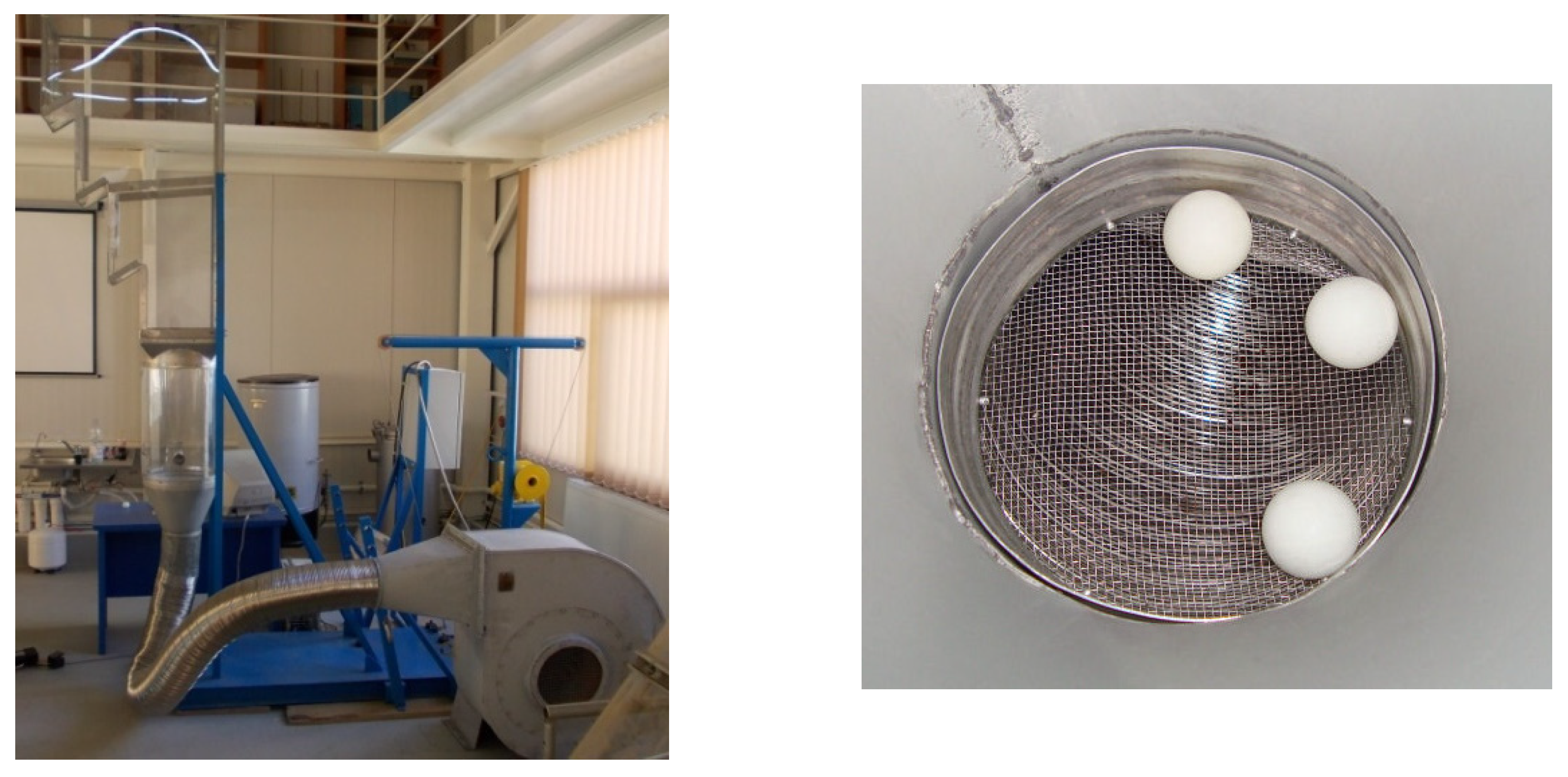
2. Materials and Methods
- -
- The values in set no. 1 correspond to the results for a solid particle with a diameter of 27 mm—there are 9 values;
- -
- The values in set no. 2 correspond to the results for a solid particle with a diameter of 35 mm—there are 9 values;
- -
- The values in set no. 3 correspond to the results for a solid particle with a diameter of 47 mm—there are 9 values;
- -
- The values in set no. 4 correspond to the results for a solid particle with a diameter of 56 mm—there are 6 values;
- -
- The average instantaneous velocity (m/s);
- -
- Average angular velocity (rad/s).
3. Results
- -
- The sphericity parameter, which depends on the type of particle used in the experimental determinations;
- -
- The value of the velocity of the airflow that passes through the vertical tubing depends on the operating mode of the installation used;
- -
- and the output parameters:
- -
- The average instantaneous velocity (Figure 2);
- -
- The average angular velocity (Figure 3).


4. Identifying the Mathematical Equation
- Experimentally obtained values are entered into an Excel 97-2003 file;
- The Excel file was inserted into Table Curve 3D (the application allows for such an insertion [41]);
- The three axes’ parameters are chosen, the input parameters are entered on the OX and OY axes, and the tracked parameter is entered on the OZ axis.;
- -
- A total of 338 equations were obtained for the average value of the instantaneous velocity for the particle with a diameter of 27 mm (maximum number of the equation), and 178 equations were generated for the particle with a diameter of 56 mm (minimum number of the equation);
- -
- In the case of average angular velocity, 444 equations were generated for the particle with a diameter of 36 mm (maximum number of equation), and 178 equations were generated for the particle with a diameter of 56 mm (minimum number of equation).
- 5.
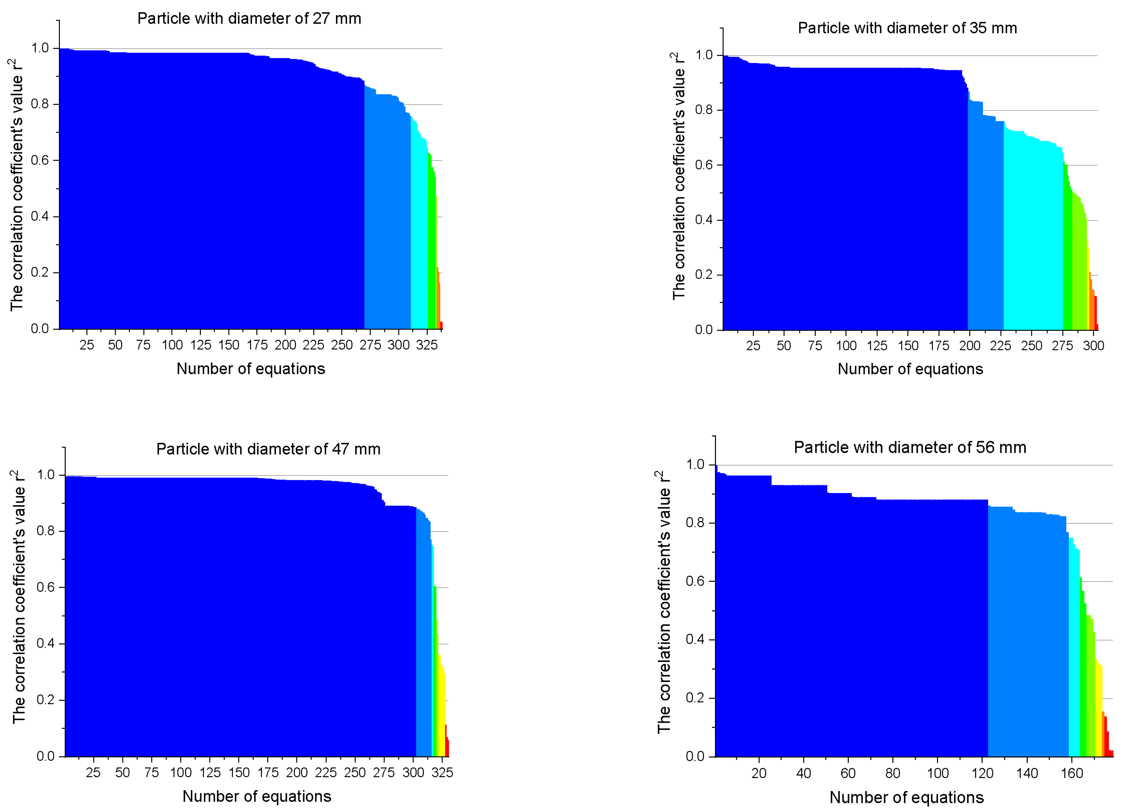
- The resulting equations are categorized based on the r2 correlation coefficient value. (Figure 7).
- -
- The values of the coefficient r2 are distributed as follows for the parameter average value of instantaneous speed:
- ○
- The largest weighting, 74.8 percent, corresponds to r2 variation in the range 0.9–1, and the smallest weighting, 0 percent, corresponds to r2 variation in the range 0.3–0.4 for the particle with a diameter of 27 mm;
- ○
- There are 196 equations developed for the particle with a diameter of 36 mm that belong to the interval 0.9–1, and the fewest number of equations are related to the interval r2 equal to 0.3–0.4;
- ○
- This parameter’s maximum weighting is also for the interval 0.9–1, at 84.09 percent for the particle with a diameter of 47 mm, while no equations were found for the intervals 0.5–0.6, 0.1–0.2, and 0–0.1;
- ○
- The maximum number of equations were formed for r2 in the range 0.8–0.9, accordingly 96 equations, for the final dimension of the examined particle, the diameter of 56 mm, while no equations were generated in the range 0.2–0.3.
- -
- The values of the coefficient r2 are distributed as follows, for the value of the average angular velocity:
- ○
- A maximum of 173 equations for the range of 0.8–0.9 and a minimum of 2 equations for the range 0.2–0.3 were created for the particle with a diameter of 27 mm;
- ○
- The largest weighting, 82.2 percent, corresponds to r2 variation in the range 0.9–1 for the particle with a diameter of 36 mm, while the smallest weighting, 0.45 percent, corresponds to r2 variation in the range 0.3–0.4;
- ○
- A maximum of 205 equations corresponding to r2 variation in the range 1–0.9 and a minimum of 0 equations corresponding to r2 variation in the range 0.3–0.4 were discovered for the particle with a diameter of 47 mm;
- ○
- A total of 81 equations for r2 in the range 0.8–0.9 were developed for the particle with a diameter of 56 mm, which indicates the interval with the most equations. For r2 between 0.6–0.7 and 0.5–0.6, no equations are generated in the intervals.
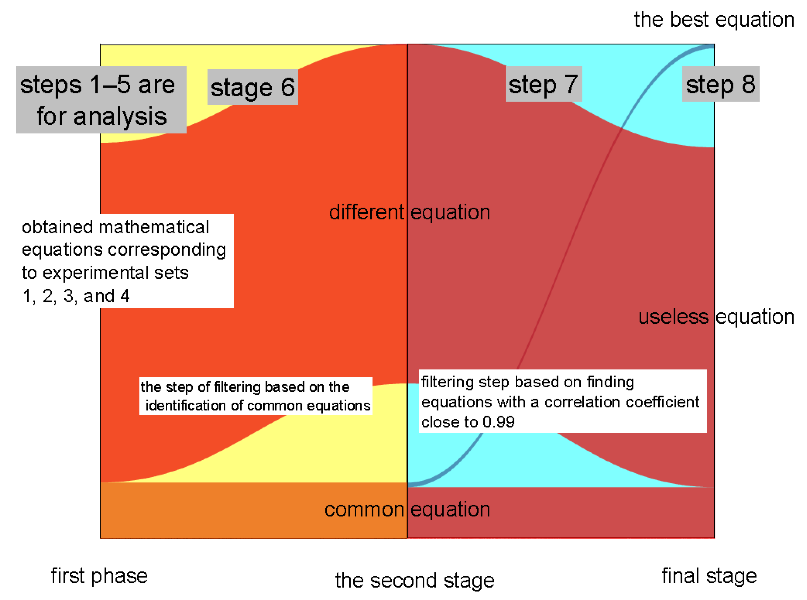
- 6.
- The next stage was to look for equations that are common (the COUNTIF function from Excel was used). The group corresponding to the experimental set with the greatest number of equations is identified at this step:
- a.
- There are 338 equations relating to the set of tests for the particle with a diameter of 27 mm, for the variation of the linear average velocity;
- b.
- There are 444 equations relating to the set of experiments for the particle with a diameter of 36 mm, for the variation of the average angular velocity.
- -
- No. 3 denotes that the reference set’s equation can also be found in the other three sets of equations;
- -
- No. 2 indicates that the reference set equation can only be found in two sets of equations;
- -
- No. 1 indicates that the reference set equation can only be found in a set of equations;
- -
- No. 0 indicates that the reference set’s equation is not found in any other set of equations.
- 7.
- An analysis of the common equations is carried out in order to choose the equations in which the correlation coefficient r2 is as close to 0.99 as possible (for all sets of experiments). INDEX, SUM, and MAX functions from Excel were used to perform this filtering step (Figure 9). Only four equations were discovered at this point for both parameters studied.
- 8.
- Following that, a visual examination of each term of the mathematical equation will be carried out in accordance with the requirements shown in Figure 4.
- -
- The number of equations identified in stage 4 is presented in the first stage;
- -
- The common equations are highlighted in the second stage, according to stage 6 of the methodology (Figure 8, No. 3);
- -
- After the filtering stage, there are a number of equations that match the criteria and may be used to describe the mathematical relationship between the input and output parameters.
5. Selecting the Best Mathematical Equation
6. Discussion
7. Conclusions
- -
- An average of 287 mathematical equations were generated for the average instantaneous velocity parameter, and another 312 mathematical equations were generated for the average angular velocity parameter.
- -
- For each parameter, only four equations could be identified using the process for selecting a generalized mathematical equation.
- -
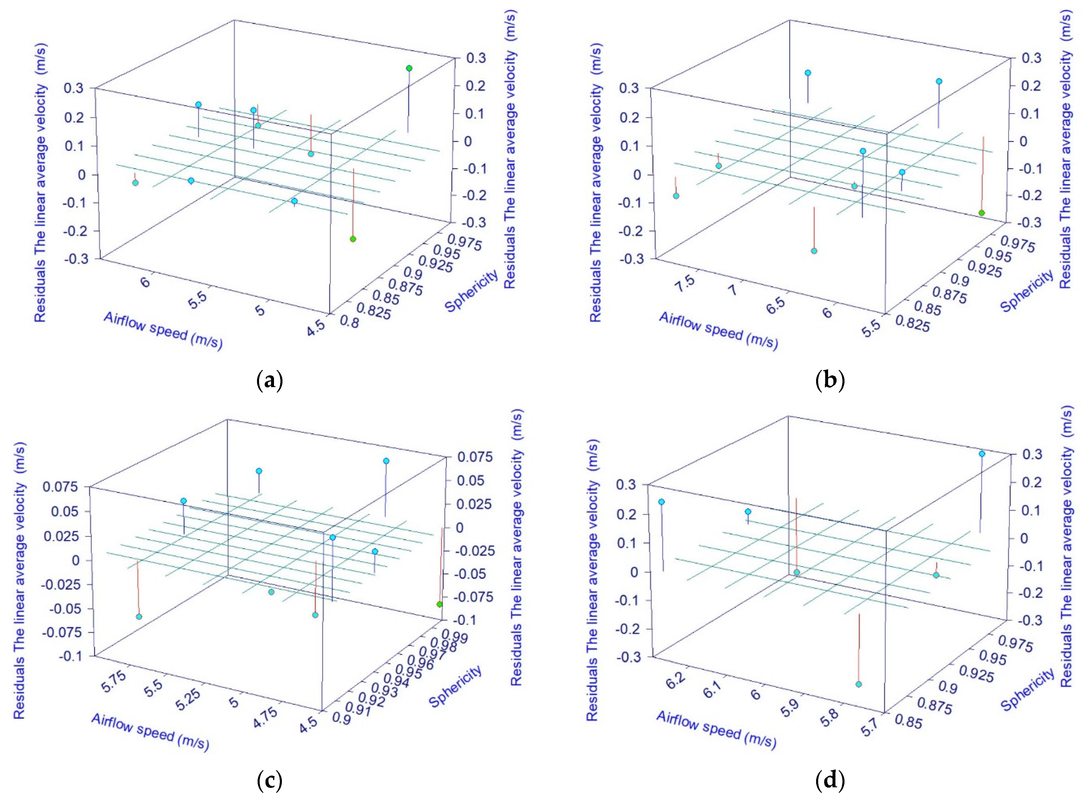
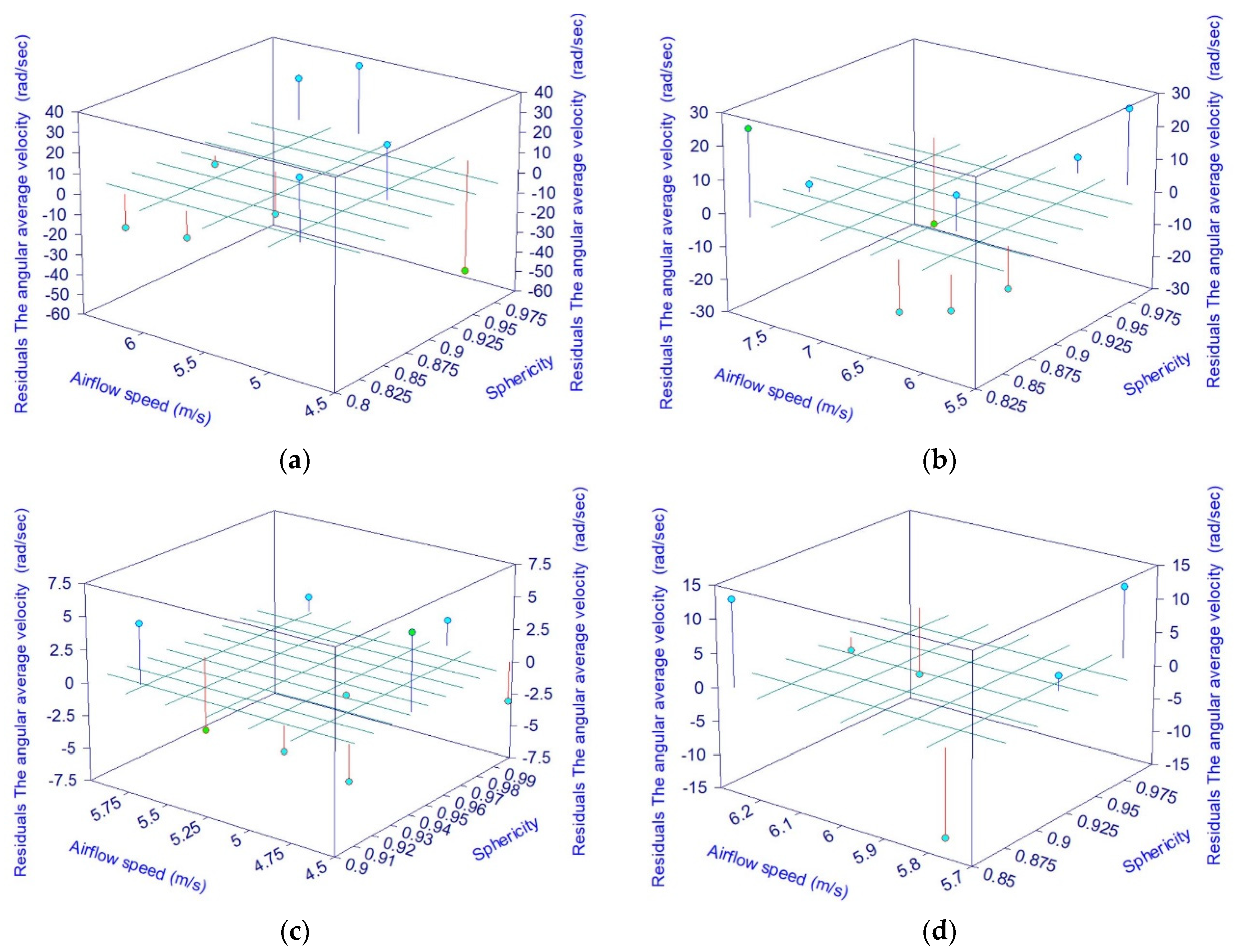
- After examining the differences between experimental and mathematical equation values, it was determined that:
- ○
- The highest variation in the average instantaneous velocity parameter is 0.28 m/s, whereas the lowest difference is 0.003 m/s.
- ○
- The highest variation in the average angular velocity parameter is 56.36 rad/s, and the smallest difference is 0.059 rad/s.
Author Contributions
Funding
Institutional Review Board Statement
Informed Consent Statement
Data Availability Statement
Conflicts of Interest
References
- Abdel, M.M.; Sameh, M.S. Development of risk assessment model for equipment within the petroleum industry. IFAC-PaperOnLine 2016, 28–49, 037–042. [Google Scholar]
- Al-Shammari, M.H.J.; Algretawee, H.; Al-Aboodi, A.H. Using eight crops to show the correlation between Paucity irrigation and yield reduction of Al-Hussainiyah irrigation project in Karbala, Iraq. J. Eng. 2020, 2020, 4672843. [Google Scholar] [CrossRef]
- Azmi, A.; Jasni, J.; Azis, N.; Kadir, M.Z.A.A. Evolution of transformer health index in the form of mathematical equation. Renew. Sustain. Energy Rev. 2017, 76, 687–700. [Google Scholar] [CrossRef]
- Flumignan, D.L.; Rezende, M.K.A.; Comunello, E.; Fietz, C.R. Empirical methods for estimating reference surface net radiation from solar radiation. Eng. Agrícola 2018, 38, 32–37. [Google Scholar] [CrossRef] [Green Version]
- Graba, M. About determining the coefficient η for J-integral for SEN(B) specimens. In Proceedings of the 3rd National Conference on Current and Emerging Process Technologies—Concept, Tamil Nadu, India, 25 January 2020. [Google Scholar]
- Kjurkchieva, D.; Khruzina, T.; Dimitrov, D.; Groebel, R.; Ibryamov, S.; Nikolov, G. The newly discovered cataclysmic star with the deepest eclipse. Astron Astrophys. 2015, 584, A40. [Google Scholar] [CrossRef] [Green Version]
- Rahman, L.; Shinwari, Z.K.; Iqrar, I.; Rahman, L.; Tanveer, F. An assessment on the role of endophytic microbes in the therapeutic potential of Fagonia indica. Ann. Clin. Microbiol. Antimicrob. 2017, 16, 53. [Google Scholar] [CrossRef] [PubMed]
- Saruchi, S.A.; Mohammed Ariff, M.H.; Zamzuri, H.; Hassan, N.; Wahid, N. Artificial neural network for modelling of the correlation between lateral acceleration and head movement in a motion sickness study. IET Intell. Transp. Syst. 2018, 13, 340–346. [Google Scholar] [CrossRef]
- Paterson, C.; Clevers, H.; Bozic, I. Mathematical model of colorectal cancer initiation. Proc. Natl. Acad. Sci. USA 2020, 117, 20681–20688. [Google Scholar] [CrossRef]
- Pang, T. Human body movement coupling model in physical education class in the educational mathematical equation of reasonable exercise course. Appl. Math. Nonlinear Sci. 2021, 1–8. [Google Scholar] [CrossRef]
- Goh, E.G.; Noborio, K. Erratum to: An improved heat flux theory and mathematical equation to estimate water vapor advection as an alternative to mechanistic enhancement factor. Transp. Porous Media 2016, 112, 545–547. [Google Scholar] [CrossRef] [Green Version]
- Watanabe, S.; Kitawaki, T.; Oka, H. Mathematical equation of fusion index of tetanic contraction of skeletal muscles. J. Electromyogr. Kinesiol. 2010, 20, 284–289. [Google Scholar] [CrossRef] [Green Version]
- Savin, C.; Panainte, M.; Mosnegutu, E.; Nedeff, V. Amestecarea Produseor Agroalimentare; Tehnopress: Iasi, Romania, 2006. [Google Scholar]
- Panainte, M.; Mosnegutu, E.; Savin, C.; Nedeff, V. Mărunţirea Produselor Agroalimentare; Meronia: Bucharest, Romania, 2005. [Google Scholar]
- Tenu, I. Operatii și Aparate in Industria Alimentara; Ion Ionescu de la Brad: Iasi, Romania, 2008; Volume 1. [Google Scholar]
- Nedeff, V.; Moşneguţu, E.; Panainte, M.; Savin, C.; Măcărescu, B. Separarea Amestecurilor de Particule Solide in Curenţi de Aer Verticali; Editua Alma Mater: Bacău, Romania, 2007. [Google Scholar]
- He, Y.; Wang, H.; Duan, C.; Song, S. Airflow fields simulation on passive pulsing air classifiers. J. S. Afr. I Min. Metall. 2005, 105, 525–531. [Google Scholar]
- Sun, Z.P.; Sun, G.G.; Liu, J.X.; Yang, X.N. CFD simulation and optimization of the flow field in horizontal turbo air classifiers. Adv. Powder Technol. 2017, 28, 1474–1485. [Google Scholar] [CrossRef]
- Ristea, M. Contributions to the Study of Aerodynamic Separation Process of Solids Particles Mixture with Application in Food Industry (Contribuții la Studiul Procesului de Separare Aerodinamică a Amestecurilor de Particule Solide cu Aplicații în Industria Alimentară). Ph.D. Thesis, Universitatea “Vasile Alecsandri”, Bacău, Romania, 2014. [Google Scholar]
- Nedeff, V.; Mosnegutu, E.; Panainte, M.; Ristea, M.; Lazar, G.; Scurtu, D.; Ciobanu, B.; Timofte, A.; Toma, S.; Agop, M. Dynamics in the boundary layer of a flat particle. Powder Technol. 2012, 221, 312–317. [Google Scholar] [CrossRef]
- Yu, Y.; Liu, J.X.; Zhang, K. Establishment of a prediction model for the cut size of turbo air classifiers. Powder Technol. 2014, 254, 274–280. [Google Scholar] [CrossRef]
- Petit, H.A.; Irassar, E.F.; Barbosa, M.R. Evaluation of the performance of the cross-flow air classifier in manufactured sand processing via CFD-DEM simulations. Comput. Part. Mech. 2018, 5, 87–102. [Google Scholar] [CrossRef]
- Mosnegutu, E.; Nedeff, V.; Ristea, M.; Ciobanu, E. A method for the study of the solid particles behavior in a vertical air flow. In Proceedings of the Process Equipment Conference (EPI-60), Bucureşti, Romania, 16 May 2014; pp. 50–55. [Google Scholar]
- Peng, S.; Wu, Y.; Tao, J.; Chen, J. Airflow velocity designing for air classifier of manufactured sand based on CPFD method. Minerals 2022, 12, 90. [Google Scholar] [CrossRef]
- Nedeff, V.; Mosnegutu, E.; Panainte, M.; Savin, C.; Macarescu, B. Study of a solid particle behaviour in a vertical ascending airflow. Rev. Chim. 2007, 58, 1285–1290. [Google Scholar]
- Zeng, Y.; Zhang, S.; Zhou, Y.; Li, M. Numerical Simulation of a flow field in a turbo air classifier and optimization of the process parameters. Processes 2020, 8, 237. [Google Scholar] [CrossRef] [Green Version]
- Ageev, A.A.; Yakhontov, D.A.; Kadyrov, T.F.; Farakhov, M.M.; Lapteva, E.A. Mathematical equation of dispersed phase gas separation in a combined equipment. Chem. Petrol. Eng. 2019, 55, 611–618. [Google Scholar] [CrossRef]
- Hwang, D.H.; Han, J.H.; Lee, J.; Lee, Y.; Kim, D. A mathematical equation for the separation behavior of a split type low-shock separation bolt. Acta Astronaut 2019, 164, 393–406. [Google Scholar] [CrossRef]
- Ibyatov, R.I.; Kholpanov, L.P.; Akhmadiev, F.G.; Fazylzyanov, R.R. Mathematical modeling of phase separation of a multiphase medium. Theor. Found Chem. En+ 2006, 40, 339–348. [Google Scholar] [CrossRef]
- Orlov, A.; Ushakov, A.; Sovach, V. Mathematical modeling of nonstationary separation processes in gas centrifuge cascade for separation of multicomponent isotope mixtures. In Proceedings of the MATEC Web of Conferences, Cape Town, South Africa, 1 February 2016; pp. 1–5. [Google Scholar]
- Orlov, A.; Ushakov, A.; Sovach, V. Mathematical equation of nonstationary hydraulic processes in gas centrifuge cascade for separation of multicomponent isotope mixtures. In Proceedings of the Thermophysical Basis of Energy Technologies (Tbet-2016), MATEC Web of Conferences 92, Tomsk, Russia, 26–28 October 2017; pp. 1–4. [Google Scholar]
- Song, J.F.; Hu, X.F. A mathematical equation to calculate the separation efficiency of streamlined plate gas-liquid separator. Sep. Purif. Technol. 2017, 178, 242–252. [Google Scholar] [CrossRef]
- Szwast, M.; Szwast, Z. A Mathematical equation of membrane gas separation with energy transfer by molecules of gas flowing in a channel to molecules penetrating this channel from the adjacent channel. Chem. Process. 2015, 36, 151–169. [Google Scholar] [CrossRef] [Green Version]
- Chitimus, A.D.; Nedeff, V.; Sandu, I.; Radu, C.; Mosnegutu, E.; Sandu, I.G.; Barsan, N. Mathematical modeling for the absorption capacity of heavy metals from the soil in the case of phragmites australis plant species. Rev. Chim. 2019, 70, 2545–2551. [Google Scholar] [CrossRef]
- Betz, M.; Gleiss, M.; Nirschl, H. Effects of Flow baffles on flow profile, pressure drop and classification performance in classifiers. Processes 2021, 9, 1213. [Google Scholar] [CrossRef]
- Cobzaru, C.; Marinoiu, A.; Apostolescu, G.A.; Tataru-Farmus, R.E.; Cernatescu, C. Mathematical modeling for kinetics of fe3+ exchange on pretreated analcime. Rev. Roum. Chim. 2019, 64, 403–407. [Google Scholar] [CrossRef]
- Radulescu, G.M.T.; Radulescu, A.T.G.; Radulescu, M.V.G.; Nas, S. Mathematical modelling of the bridges structural monitoring II. J. Appl. Eng. Sci. 2015, 5, 91–99. [Google Scholar] [CrossRef] [Green Version]
- Barsan, N.; Joita, I.; Stanila, M.; Radu, C.; Dascalu, M. Modelling wastewater treatment process in a small plant using a sequencing batch reactor (SBR). Environ. Eng. Manag. J. 2014, 13, 1561–1566. [Google Scholar] [CrossRef]
- Zhou, Y.; Shen, W. Numerical simulation of particle classification in new multi-product classifier. Chem. Eng. Res. Des. 2022, 177, 484–492. [Google Scholar] [CrossRef]
- Moșneguțu, E.; Nedeff, V.; Bârsan, N.; Rusu, D. The influence of air velocity on the behavior of a solid particle displacement in a vertical path. Stud. Res. Sci. Chim. Ing. Chim. Biotehnol. Ind. Aliment. 2018, 19, 431–441. [Google Scholar]
- Moşneguţu, E.; Nedeff, V.; Panainte, M.; Burca, G. Theoretic study concerning the behavior on solid particle into vertical airflow. In Proceedings of the 5th International Conference Research and Development in Mechanical Industry RaDMI 2005, 4–7 September 2005; pp. 744–747. [Google Scholar]
- Nedeff, V.; Lazar, G.; Agop, M.; Mosnegutu, E.; Ristea, M.; Ochiuz, L.; Eva, L.; Popa, C. Non-linear behaviours in complex fluid dynamics via non-differentiability. Separation control of the solid components from heterogeneous mixtures. Powder Technol. 2014, 269, 452–460. [Google Scholar] [CrossRef]
- Corporation Origine OriginPro 2019b, Version 9.6.5.169. Available online: https://www.originlab.com/ (accessed on 13 March 2020).
- SYSTAT Software Inc. TableCurve 3D, Version 4.0. Available online: https://systatsoftware.com/downloads/download-tablecurve-3d/ (accessed on 13 March 2020).


| The Solid Particle Diameter | Sphericity * | Airflow Velocity (m/s) |
|---|---|---|
| 27 mm | 1 | 4.896 m/s; 5.775 m/s; 6.277 m/s |
| 0.90856 | 4.896 m/s; 5.775 m/s; 6.277 m/s | |
| 0.81781 | 4.896 m/s; 5.775 m/s; 6.277 m/s | |
| 35 mm | 1 | 5.775 m/s; 6.277 m/s; 7.784 m/s |
| 0.88118 | 5.775 m/s; 6.277 m/s; 7.784 m/s | |
| 0.82946 | 5.775 m/s; 6.277 m/s; 7.784 m/s | |
| 47 mm | 1 | 4.519 m/s; 4.896 m/s; 5.775 m/s |
| 0.94231 | 4.519 m/s; 4.896 m/s; 5.775 m/s | |
| 0.90911 | 4.519 m/s; 4.896 m/s; 5.775 m/s | |
| 56 mm | 1 | 5.775 m/s; 6.277 m/s |
| 0.94433 | 5.775 m/s; 6.277 m/s | |
| 0.85499 | 5.775 m/s; 6.277 m/s |
| Diameter of Solid Particle (mm) | Source of Sampling | The Value of the Correlation Coefficients r2 |
|---|---|---|
| 27 | the average instantaneous velocity | 0.98404352 |
| 35 | 0.954536506 | |
| 47 | 0.991563069 | |
| 56 | 0.8806499 | |
| 27 | the average angular velocity | 0.883216778 |
| 35 | 0.918608489 | |
| 47 | 0.992395157 | |
| 56 | 0.868026975 |
| Diameter of Solid Particle (mm) | The Constant Values | ||||
|---|---|---|---|---|---|
| a | b | c | d | e | |
| The average instantaneous velocity | |||||
| 27 | −50.23223724 | −11.95975744 | −34.97830761 | 17.47111956 | −1.415462687 |
| 35 | −49.20607684 | −0.92288797 | 16.90007259 | 15.17783217 | −1.067222164 |
| 47 | −1.820559781 | 0.557052644 | 52.79511238 | 0.978623048 | 0.001785313 |
| 56 | −28.8899824 | −15.53346772 | −52.68311297 | 9.116452615 | −0.640957447 |
| The average angular velocity | |||||
| 27 | −1559.120656 | −1551.787458 | −4519.318535 | 561.1160605 | −41.90513018 |
| 35 | −645.2588717 | −524.764458 | 574.9907661 | 198.8608978 | −11.88403605 |
| 47 | −3171.846461 | −519.4420102 | 436.8999213 | 1245.268354 | −114.7711104 |
| 56 | −999.2614963 | −306.5043777 | −297.4052482 | 297.6328447 | −18.55319149 |
| Difference | Diameter of the Solid Particle (mm) | |||
|---|---|---|---|---|
| 27 | 35 | 47 | 56 | |
| the average instantaneous velocity (m/s) | ||||
| maximum | −0.2541 | −0.2841 | −0.0838 | −0.2843 |
| minimum | 0.2334 | 0.2199 | 0.0624 | 0.2843 |
| the average angular velocity (rad/s) | ||||
| maximum | −56.3629 | −28.2754 | −5.7759 | −12.8663 |
| minimum | 35.0704 | 26.07388 | 5.8351 | 12.8662 |
Publisher’s Note: MDPI stays neutral with regard to jurisdictional claims in published maps and institutional affiliations. |
© 2022 by the authors. Licensee MDPI, Basel, Switzerland. This article is an open access article distributed under the terms and conditions of the Creative Commons Attribution (CC BY) license (https://creativecommons.org/licenses/by/4.0/).
Share and Cite
Mosnegutu, E.; Panainte-Lehadus, M.; Nedeff, V.; Tomozei, C.; Barsan, N.; Chitimus, D.; Jasinski, M. Extraction of Mathematical Correlations Applied in the Aerodynamic Separation of Solid Particles. Processes 2022, 10, 1234. https://doi.org/10.3390/pr10071234
Mosnegutu E, Panainte-Lehadus M, Nedeff V, Tomozei C, Barsan N, Chitimus D, Jasinski M. Extraction of Mathematical Correlations Applied in the Aerodynamic Separation of Solid Particles. Processes. 2022; 10(7):1234. https://doi.org/10.3390/pr10071234
Chicago/Turabian StyleMosnegutu, Emilian, Mirela Panainte-Lehadus, Valentin Nedeff, Claudia Tomozei, Narcis Barsan, Dana Chitimus, and Marcin Jasinski. 2022. "Extraction of Mathematical Correlations Applied in the Aerodynamic Separation of Solid Particles" Processes 10, no. 7: 1234. https://doi.org/10.3390/pr10071234