
New Directions in Modeling and Computational Methods for Complex Mechanical Dynamical Systems


Abstract
:1. Introduction
- (1)
- The methodology is developed for a non-uniform shell and two particles of zero mass are used instead of one. This greatly simplifies the formulation of the problem from that obtained in Ref. [29] and the formulation of the equations of motion and the equations of constraint. It also makes the computations more efficient.
- (2)
- The theory of constrained motion with singular mass matrices is used to obtain the final equations of motion of the system [15,16,30,31]. This theory requires a certain condition to be satisfied in order to yield the correct equations of motion for the physical system. In Ref. [29] this condition was only computationally confirmed for the parameters chosen in the numerical example presented there. Here, we show that the condition is analytically satisfied, thereby placing the approach on a firm mathematical footing. This allows us to obtain the explicit closed form equations of motion for the shell moving over an arbitrarily prescribed surface.
- (3)
- Computational results that show the motion of the shell on a complex unsymmetrical multi-dimpled bowl-shaped surface with an unsymmetrical cross-section are obtained, showing vast qualitative differences in its motion and sensitive dependence on initial conditions.
- (4)
- Analytical equations for the reaction of the surface to the motion of the shell from the determination of the generalized forces of constraint are explicitly obtained. That is, besides obtaining the coordinates that describe the configuration of the system at each time instant and the velocities of these coordinates as done in Ref. [28], the generalized forces acting on the spherical shell at its point of contact with the surface are also determined. Thus, the reaction forces exerted by the surface are therefore explicitly obtained. This permits the minimum coefficient of friction required to sustain the motion of the shell over the surface, without any slippage, to be determined.
- (5)
- The effects of the initial orientation and the initial spin velocity of the shell—the component of the initial angular velocity normal to the surface—are investigated in considerable detail, showing that they have a significant effect on its motion.
- (6)
- A further constraint that prevents the shell to have any spin velocity is investigated. Its effect on the motion of the shell, and especially on the reaction forces that it brings about, is investigated in some detail.
2. Analytical Results
2.1. Description of the Unconstrained Multi-Body System
2.2. Description of the Constraints
- (1)
- The use of quaternions to describe the rotational dynamics of the shell;
- (2)
- The description of the location of the two zero-mass particles, one placed at the point of contact P between the shell and the surface and the other at the center, O, of ;
- (3)
- The constraints relevant to the physical conditions that must be satisfied by the shell to roll without slipping on the surface;
- (4)
- Additional constraints that might be redundant but are consistent with all the other existing constraints, and/or constraints that may be added to the system to, for example, further physically constrain the motion of the shell .
- (1)
- Quaternion ConstraintThe constraint on the four-vector u, as mentioned before, is described byA suitable form of constraint can be obtained by taking the second time derivative of Equation (15) to yieldWe call the ‘Quaternion Constraint’.
- (2)
- Location of the two zero-mass particles at P and O
- (i)
- Location of the zero-mass particle at PThe first zero-mass particle is co-located at the point P that lies at the point of contact between the shell and the surface, and therefore its coordinate must satisfy the equation of the surface. This leads to the constraintwhich we shall refer to as the ‘Surface Constraint’.As before, the second time derivative of Equation (17) in term of k, defined in Equation (13), is given bynoting that the matrix is symmetric.
- (ii)
- Location of the zero-mass particle at OFor the second zero-mass particle to be co-located with the point O, which is the geometric center of the shell (see Figure 2), the distance OP must be r and O must lie along the normal to the surface at P. Hence, we obtain the relationWe call this the ‘Tangency Constraint’. Again, taking the second derivative of Equation (19) with respect to time t, we can writeThe matrix and the three by one column vector are obtained in Appendix A aswhere the Jacobian , and the expressions for and are given in Appendix A.
- (3)
- Physical Constraints
- (i)
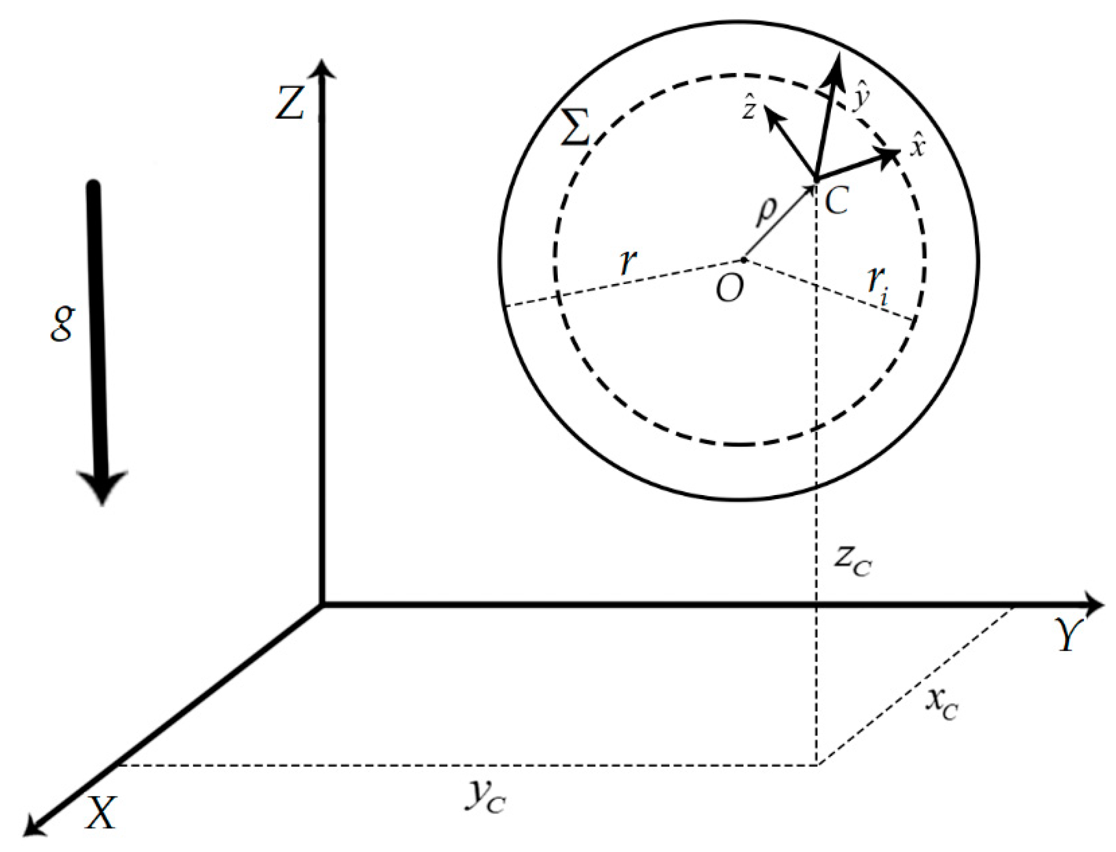
- Constraint onAs seen from Equation (10), the coordinate of the center of mass C of the shell in the unconstrained system is uncoupled from the coordinates u, , . However, when the shell rolls over the surface , depends on the (rotational) orientation of the shell and the location of the point of contact (or alternately as seen from Equation (12), the location of the point O). The zero-mass particle co-located at O simplifies this relation and we havewhere is the active rotation matrix, which can be written in terms of the quaternion components asand is the vector that starts from the center of the shell O and points to the center of mass C of the shell; its components are measured in the body-fixed coordinate frame and are therefore constant and they depend on the distribution of the mass of in the shell (see Figure 1). We call the constraint, , the ‘Geometric Center Constraint’.We write the constraint Equation (22) in suitable form by taking its second derivative with respect to time. Defining whereand the second derivative of Equation (22) can be written aswhich can be recast in the form
- (ii)
- The Rolling No-Slip ConstraintThe shell rolling on the surface without slipping requires the non-holonomic constraintto be satisfied at each instant of time t. We note that the normal to the surface is and it is therefore a function of the time, t, as the shell rolls over the surface. The active rotation matrix is given in Equation (23). The matrix is the three by three skew-symmetric matrix obtained from the components of the unit three-vector in the XYZ coordinate frame in Equation (14); it is given byThis notation of a tilde above a three-vector to denote the skew-symmetric matrix of its components shown on the right hand side of (28) will be used throughout this paper. Equation (27) states that the instantaneous velocity of the point on the shell that touches the surface is zero. The second term in Equation (27) is the relative velocity of this point while the shell is rotating with angular velocity . The three-vector contains the components of the angular velocity in the body-fixed coordinate frame.Differentiating Equation (27) twice with respect to time t, we obtainwhich, upon noting that , can be rewritten asSince , , and , the third term on the left in Equation (30) is zero and the equation can be simplified toConstraints (16), (20), (26), (18), and (31), obtained so far, can be expressed as a system of equations in form ofwhere the matrix is an 11 by 13 matrix and vector b is an 11-vector (11 by 1). These five sets of constraint equations are sufficient to model the spherical shell rolling on the surface without slipping. It should be noted that the rows of matrix do not have to be independent and multiple consistent constraints can be imposed on the system.
- (4)
- Additional Constraints
- (i)
- Constraints Related to Known Conserved QuantitiesOne of the significant advantages of this methodology is that even additional constraints that are not independent from of the existing constraints can be added to the system. In other words, the rows of matrix need not be independent. This capability lets us make the numerical model more consistent with conserved quantities that are known to exist during the evolving motion of the system. For instance, in the modeling of a system whose energy is conserved, the energy conservation equation can be added to the rows of matrix as an additional constraint.Since there is no dissipation or injection of energy to our system, energy is conserved. Using Equations (2) and (3), the equation that states that the total amount of energy, , of the system at each instant of time t remains constant can be written asand taking the time derivative of Equation (33) gives the relationwhereHence, Equation (34) can be added to the set of constraints given in Equation (32), so that the augmented set of constraints is given by the system of equationswhere the matrix A is now 12 by 13 and the vector b is 12 by 1.
- (ii)
- No-Spin ConstraintAlthough the constraints in Equation (32) are sufficient to model the motion of the shell rolling on a prescribed surface without slipping, depending on the situation at hand, the motion of the shell can be further restricted by imposing additional constraints. For instance, the spin of the shell about the normal vector to the surface can be prevented during its rolling motion by the inclusion of an additional constraint.As shown in Appendix B, the components of the angular velocity of the shell at each instant of time in the body-frame and in the XYZ inertial frame can be expressed asandrespectively. The two three-vectors on the right hand side in the last equality in Equation (38) are orthogonal to each other since . The component of along the unit normal n to the surface is . Thus, from Equation (38) we see that the component of the angular velocity (in the inertial XYZ frame) normal to the surface is . In addition, the tangential component of the angular velocity is determined in terms of the velocity three-vector of the center O of the shell. When , the angular velocity of the shell is thus seen to depend only on the velocity of its center O.We refer to the component of the angular velocity about an axis normal to the surface as the ‘spin velocity’ of the shell throughout this paper.Noting from Equation (14) that the three-vector , we have . Thus, to constrain the shell from ‘spinning’ about the normal to the surface when it rolls, we use the non-holonomic constraint [24]The subscript ‘NS’ signifies the ‘No-Spin’ constraint. This constraint simply states that the component of the angular velocity vector along the vector n is zero during the motion of the shell. Differentiating Equation (39) twice with respect to time, we obtainThe first bracketed term on the left hand side computes to , where we have used Equation (1) in the second-last equality. Equation (40) can be rearranged asIf this additional No-Spin constraint is required to be imposed, one simply includes Equation (41) in the set of constraints given earlier in Equation (36). This gives the new set of constraint equationswhere the matrix , upon this inclusion, is now a 13 by 13 matrix and the column vector b is a 13-vector.It should be noted that in the presence of the No-Spin constraint, the energy of the constrained system is still conserved, because at each instant of time the spin about the normal n to the surface is zero and therefore there is no work done by the constraint torque about the normal; Equations (34) and (33) therefore continue to be applicable to the dynamical system.As seen above, the methodology developed here allows the easy handling of additional constraints. In a simple and straightforward manner, it permits one to determine the effect of the addition or exclusion of one or more constraints on the evolutionary dynamics of the system.
2.3. Description of the Constrained Multi-Body System
2.4. Explicit Equations of Motion
2.5. Determination of the Generalized Constraint Forces and the Generalized Reaction Provided by the Surface
3. Computational Results
3.1. Three Examples and Four Initial Shell Orientations
3.1.1. Example 1
3.1.2. Example 2
3.1.3. Example 3
4. Discussion
5. Conclusions
Supplementary Materials
Author Contributions
Funding
Data Availability Statement
Conflicts of Interest
Appendix A
Appendix B
References
- Newton, I.; Motte, A.; Chittenden, N.W. Newton’s Principia: The Mathematical Principles of Natural Philosophy; Daniel Adee: New York, NY, USA, 1850. [Google Scholar]
- Euler, L. Discovery of a New Principle of Mechanics. M’emoires De L’academie Des Sci. De Berl. 1752, 6, 185–217. [Google Scholar]
- Poincaré, H. Sur certaines solutions particulières du probléme des trois corps. Bull. Astron. 1884, 1, 65–74. [Google Scholar] [CrossRef]
- Poincaré, H. Sur le problème des trois corps et les équations de la dynamique. Acta Math. 1890, 13, 1–270. [Google Scholar]
- Lagrange, J.L. Mecanique Analytique; Mme Ve Courcier: Paris, France, 1787. [Google Scholar]
- Gauss, C.F. Uber Ein Neues Allgemeines Grundgesetz der Mechanik. J. Reine Agnew. Math. 1829, 4, 232–235. [Google Scholar]
- Gibbs, J.W. On the Fundamental Formulas of Dynamics. Am. J. Math. 1879, 2, 49–64. [Google Scholar] [CrossRef]
- Udwadia, F.E.; Kalaba, R.E. A New Perspective on Constrained Motion. Proc. R. Soc. Lond. Ser. A Vol. 1992, 439, 407–410. [Google Scholar]
- Udwadia, F.E.; Kalaba, R.E. On Motion. J. Frankl. Inst. 1993, 330, 571–577. [Google Scholar] [CrossRef]
- Udwadia, F.E.; Kalaba, R.E. Analytical Dynamics: A New Approach; Cambridge University Press: Cambridge, UK, 1996. [Google Scholar]
- Udwadia, F.E.; Kalaba, R.E. On the Foundations of Analytical Dynamics. Int. J. Non-Linear Mech. 2002, 37, 1079–1090. [Google Scholar] [CrossRef]
- Udwadia, F.E.; Kalaba, R.E. What is the General Form of the Explicit Equations of Motion for Constrained Mechanical Systems? J. Appl. Mech. 2002, 69, 335–339. [Google Scholar] [CrossRef]
- Udwadia, F.E. A New Perspective on the Tracking Control of Nonlinear Structural and Mechanical Systems. Proc. R. Soc. Lond. Ser. A Vol. 2003, 459, 1783–1800. [Google Scholar] [CrossRef]
- Udwadia, F.E.; Shutte, A.D. An Alternative Derivation of the Quaternion Equations of Motion for Rigid-Body Rotational Dynamics. ASME J. Appl. Mech. 2010, 77, 044505. [Google Scholar] [CrossRef]
- Udwadia, F.E.; Phohomsiri, P. Explicit equations of Motion for Constrained Mechanical Systems with Singular Mass Matrices and Applications to Multi-body dynamics. Proced. R. Soc. A 2006, 462, 2097–2117. [Google Scholar] [CrossRef]
- Udwadia FESchutte, A.D. Equations of Motion for General Constrained Systems in Lagrangian Mechanics. Acta Mech. 2010, 213, 111–129. [Google Scholar] [CrossRef]
- Lindelöf, E. Sur le mouvement d’un corps de revolution roulant sur un plan horizontal. Acta Soc. Sci. Fenn. 1895, 20. [Google Scholar]
- Chaplygin, S.A. On Ball’s Rolling on Horizontal Plane; Collection of Works; GITTL: Moscow, Russia, 1948; Volume 1, pp. 76–101. [Google Scholar]
- Chaplygin, S.A. On Motion of Heavy Rigid Body of Revolution on Horizontal Plane; Collection of Works; GITTL: Moscow, Russia, 1948; Volume 1, pp. 57–75. [Google Scholar]
- Kilin, A.A. The Dynamics of Chaplygin Ball: The qualitative and computer analysis. Regul. Chaotic Dyn. 2001, 6, 291–306. [Google Scholar] [CrossRef]
- Borisov, A.V.; Mamaev, I.S. Rolling of a Rigid Body on a Plane and Sphere: Hierarchy of dynamics. Regul. Chaotic Dyn. 2002, 7, 177–200. [Google Scholar] [CrossRef]
- Borisov, A.V.; Mamaev, I.S. Rolling of a Non-Homogeneous Ball over a Sphere Without Slipping and Twisting. Regul. Chaotic Dyn. 2007, 12, 153–159. [Google Scholar] [CrossRef]
- Borisov, A.V.; Kilin, A.A.; Mamaev, I.S. Rolling of a Homogeneous Ball over a Dynamically Asymmetric Sphere. Regul. Chaotic Dyn. 2011, 16, 465–483. [Google Scholar] [CrossRef]
- Borisov, A.V.; Mamaev, I.S.; Bizyaev, I.A. The Hierarchy of Dynamics of a Rigid Body Rolling without Slipping and Spinning on a Plane and a Sphere. Regul. Chaotic Dyn. 2013, 18, 277–328. [Google Scholar] [CrossRef]
- Bizyaev, I.A.; Borisov, A.V.; Mamaev, I.S. The Dynamics of Nonholonomic Systems Consisting of a Spherical Shell with a Moving Rigid Body Inside. Regul. Chaotic Dyn. 2014, 19, 198–213. [Google Scholar] [CrossRef]
- Ivanov, A.P. On Final Motions of a Chaplygin Ball on a Rough Plane. Regul. Chaotic Dyn. 2016, 21, 804–810. [Google Scholar] [CrossRef]
- Borisov, A.V.; Ivanova, T.B.; Kilin, A.A.; Mamaev, I.S. Nonholonomic rolling of a ball on the surface of a rotating cone. Nonlinear Dyn. 2019, 97, 1635–1648. [Google Scholar] [CrossRef]
- Kilin, A.A.; Pivovarova, E.N. Motion Control of a Spherical Robot Rolling on a Vibrating Plane. Appl. Math. Model. 2021, 109, 492–508. [Google Scholar] [CrossRef]
- Udwadia, F.E.; Mogharabin, N. The Use of Zero-Mass Particles in Analytical and Multi-Body Dynamics: Sphere Rolling on An Arbitrary Surface. ASME J. Appl. Mech. 2021, 88, 121006. [Google Scholar] [CrossRef]
- Udwadia, F.E.; Wanichanon, T. On General Nonlinear Mechanical Systems. Numer. Algebra Control. Optim. 2013, 3, 425–443. [Google Scholar] [CrossRef]
- Schutte, A.D.; Udwadia, F.E. New Approach to the Modeling of Complex Multi-body Dynamical Systems. J. Appl. Mech. 2011, 78, 021018. [Google Scholar]
- Udwadia, F.E.; Kalaba, R.E. An Alternate derivation of the Greville Formula. J. Optim. Theory Appl. 1994, 94, 23–28. [Google Scholar] [CrossRef]
- Udwdia, F.E. Rigid Shell Rolling on a Dimpled Bowl-Shaped Rigid Surface Example 1, In Special Issue of Processes (ISSN 2227-9717) on “Numerical Simulation of Nonlinear Dynamical Systems”. 2022. Available online: https://zenodo.org/record/6872914#.YvC-_RxBzIU (accessed on 22 July 2022).


| Case | Initial Quaternion | Initial Orientation of the Body-Fixed Frame (BFF) |
|---|---|---|
| A | No rotation of BFF with respect to the inertial frame | |
| B | BFF in Case A is rotated by counterclockwise around the -axis | |
| C | BFF in Case A is rotated by clockwise around the -axis | |
| D | 1 | The -axis of the BFF in Case A points in the direction of the normal vector to the surface. |
Publisher’s Note: MDPI stays neutral with regard to jurisdictional claims in published maps and institutional affiliations. |
© 2022 by the authors. Licensee MDPI, Basel, Switzerland. This article is an open access article distributed under the terms and conditions of the Creative Commons Attribution (CC BY) license (https://creativecommons.org/licenses/by/4.0/).
Share and Cite
Udwadia, F.E.; Mogharabin, N. New Directions in Modeling and Computational Methods for Complex Mechanical Dynamical Systems. Processes 2022, 10, 1560. https://doi.org/10.3390/pr10081560
Udwadia FE, Mogharabin N. New Directions in Modeling and Computational Methods for Complex Mechanical Dynamical Systems. Processes. 2022; 10(8):1560. https://doi.org/10.3390/pr10081560
Chicago/Turabian StyleUdwadia, Firdaus E., and Nami Mogharabin. 2022. "New Directions in Modeling and Computational Methods for Complex Mechanical Dynamical Systems" Processes 10, no. 8: 1560. https://doi.org/10.3390/pr10081560