Abstract
Currently, reducing energy consumption and fossil fuel emissions are key factors placed in the first position on the European agenda. District heating technology is an attractive solution, able to satisfy the energy and environmental goals of policymakers and designers. In line with this, a different approach to planning a district heating grid based on the optimization of building clusters is presented. The case study is Wilhelmsburg, a district of Hamburg city. This approach also investigates the usage of industrial waste heat as the grid’s heat source, which is CO2-neutral. First, the data acquisition regarding the buildings’ location and heat demand are described in detail. Based on the derived data and the source of the industrial waste heat, the district heating grid is created by clustering the buildings and connecting the obtained nodes. Furthermore, the grid’s efficiency is improved by eliminating nodes, which are too distant from the heat source, or have lower heat demand. Finally, a single building is simulated in Matlab/Simulink, showing the energy-savings and ecological results. The usage of the district heating grid saves 97.32 GWh annually, which results in financial savings of €5.83 million, and avoided CO2 emissions of 19,585 tCO2.
1. Introduction
The building sector is one of the largest energy consumers in Europe today, therefore the identification of appropriate measures to reach the European reduction target is a current challenge for policymakers and designers [1]. As a result, many interventions and measures are now forecasted using planning tools and methods [2,3]. Local energy planning has therefore gained popularity in recent years, as geographic information system (GIS) applications spread and computing power has increased [4,5]. Recently, there have been numerous strategies proposed for conserving energy in the building sector, including thermal insulation, double and triple glazing, solar shadings [6,7], the efficient usage of HVAC equipment [8], hybrid energy system [9] and using renewable energy sources [10,11]. As well as these technologies, district heating systems are another viable solution for improving energy efficiency [12] and sustainable assessment [13] in buildings. Consequently, this technology is ideal for urban areas with high thermal demand densities. Heat sources, users, and distribution networks constitute the general components of DHSs. The complexity of a DHS depends on various factors [14,15]. Starting from the beginning of this technology, it was not easy to obtain proper and coherent results in line with the real problems of a district network [14].
Many advantages of this energy system are well-known, starting from the renewable energy source inclusion [16] to positive environmental impacts, also for improving the outdoor comfort for citizens [17,18]. Due to its relevant benefits, different works were developed during the last years to improve its capabilities, such as optimizing the operation of the thermal plants [19] and the supply temperature [20] or the settings of the pumping system [21]. Those approaches are often focused on specific components or issue of the DH, missing a global approach to plan the entire network. Therefore, there is still an urgent call to develop and investigated affordable approach to design the district heating in different urban areas [22,23,24]. The two most famous planning methods available in literature are the Danish method [25] and the German method [26]. In both methods, smaller branches are merged into bigger branches and the heat loads of the removed branches are incorporated into the preserved branches. Among this, Guelpa et al. [27] proposed a method to increase the performance of district heating minimizing the thermal peaks. A clustering approach is also involved to optimize the pipe grid. Results demonstrate an average reduction of the thermal peak load up to 14% thanks to this optimization. Another work [28] is focused on optimizing the multi-source energy plant sizing using different climatic scenarios, using Matlab for modelling the environment understudy. As well, Widen and Aberg [29] developed a fixed model structure (FMS) that requires only general information about DH systems for cost-optimization studies. The results demonstrate the usefulness of the FMS for DH system optimisation studies, and that increased building energy efficiency leads to a reduction in fossil fuel and biomass consumption.
A few papers have been published on multi-source production plants or distribution hubs and how to expand or redesign a distribution hub to connect new consumers to it. Among this, biomass-based district-heating networks, which represents the basis of Italian industry’s successful production, are designed using a system optimisation approach [30]. Instead, Burer et al. [31] proposed an optimized district heating and cooling plant providing heat and power to a small number of residential buildings, to minimize cost and CO2 emissions. According to Corrado et al. [32], heat pumps, wood boilers, condensing boilers, and solar energy (thermal and photovoltaic) can be combined to generate energy. Cogeneration with solar energy and wind energy was combined by Sontag et al. [33]. An interesting study developed by Trillat et al. [34], integrated CHP with an absorption chiller and desiccant cooling; while Lee et al. [35] studied the integration of solar water heating, solar photovoltaic, ground source heat pumps, electric chillers, and gas boilers into an integrated renewable energy system.
In this framework, this study aims to fulfill this field of research proposing a different approach to connect existing district heating with new one, optimizing the building clustering. In fact, few papers explore the issue of expanding or redesigning a DHS to connect new consumers to multi-source production plants. The developed method is applied to a district of Hamburg, named Wilhelmsburg. Industrial waste heat is used as heat source, which is CO2-neutral. Based on the data acquisition, the district heating grid is created by clustering the buildings and connecting the obtained nodes, also using GIS technology. The grid of the network is improved, cleaning and reducing the branches and nodes wherein the heat demand is not so relevant. To show the advantages of this approach, a single building is simulated with Matlab/Simulink. Results underlined the financial and ecological benefits not only for the building case study, but for the entire district heating network.
2. Materials and Methods
2.1. Building Location and Heat Demand Data
Firstly, the data acquisition and allocation regarding the buildings’ location and heat demand are presented in detail. It is necessary to acquire detailed information on the buildings’ location, area, and heat demand in the district, to model a realistic heating grid. The averaged and assumed building properties are not sufficient, since the location and heat demand determine the characteristics of the heating grid. Furthermore, yearly averaged heat demand data cannot take the essential seasonal differences in the heating behavior into account. The buildings’ location and area are acquired from the open-source project OpenStreetMap [36], where a polygon spanning the district, or an arbitrary area can be selected and exported. The data file contains information on buildings, land use, natural objects, places, points, railways, roads, and waterways in the selected area. The land use highlights the usage of the area within the polygon. This land use is of varying types, e.g., residential, commercial, but also grass or farmland. For this project, only the buildings and the land use are considered. The data is imported into the software QGIS, where the geoinformation is stored and viewed, and new variables are calculated.
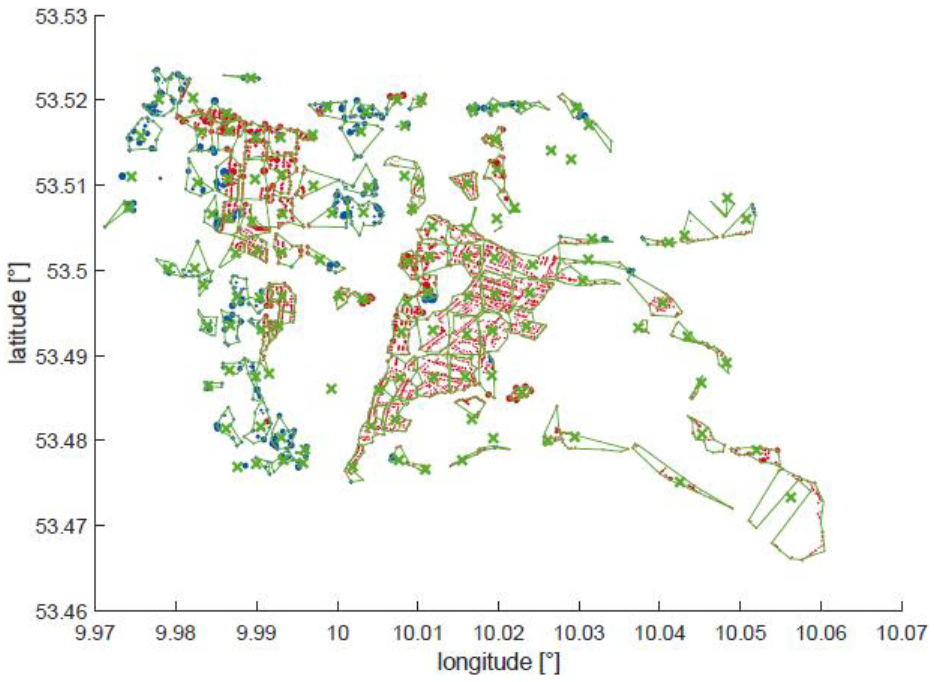
Table 1 shows exemplary fictional building data, here for a house and a commercial building. Each building has a unique ID, a type, an area, and a longitudinal and latitudinal coordinate. Here, the variable x_value denotes the longitude of the building’s center, and y_value the latitude. In Wilhelmsburg, the longitude ranges from xmin = 9.9707° to xmax = 10.0610°, and the latitude ranges from ymin = 53.4615° to ymax = 53.5239°. The type of a building is often not declared, and hence the land use is considered. For that, the buildings’ information is intersected with the land use data and hence each building is assigned its land use type, which is used whenever the building’s type is unknown. Subsequently, the types are matched to their corresponding categories, i.e., the category accommodation contains, amongst others, the types of houses, apartments, and residential. Thereby, the buildings can be summarized more broadly. Figure 1 shows real exemplary building data from Wilhelmsburg. Here, accommodational buildings are indicated in red and commercial buildings in blue. The extracted data contains the information on 6.129 buildings in Wilhelmsburg. In this manuscript, only accommodation and commercial buildings are considered, because the other categories, such as civic or religious, are miscellaneous and can hence not be easily considered regarding their heat demand.

Table 1.
Exemplary, fictional building data extracted in QGIS.
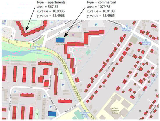
Figure 1.
Exemplary building data for an apartment (red) and a commercial (blue) building.
The heat demand for the accommodational and commercial buildings is obtained from the Wärmekataster Hamburg (heat registry Hamburg) [37]. The registry provides the heat demand and geoinformation of accommodational and commercial buildings in Hamburg. For data security reasons, the buildings are allocated in clusters of minimum 5 buildings. Hence, the heat demand cannot be matched to a single, unique building, though applying the same intersection as used for the land use matches the heat demand to each building. Some buildings are not listed in the registry and are thus outside any cluster, so the broader block of buildings is used. The available information contains:
- The specific annual heat demand for accommodational buildings in the cluster [kWh/(y m2)]
- The absolute annual heat demand for all buildings in the cluster [kWh/y]
- The area of accommodational buildings in the cluster [m2]
- The area of commercial buildings in the cluster [m2]
To calculate the absolute heat demand of each building, the specific heat demand for accommodational and commercial buildings is needed. The specific heat demand for accommodational buildings qspec,acc is already listed in the registry’s data, whereas the specific heat for commercial buildings qspec,com can be calculated using qspec,acc, the total absolute heat demand qabs,tot, the area of accommodational buildings Aacc and the area of commercial buildings Acom:
If the specific heat demand cannot be retrieved for a building, the heat demand of the building from the same category with the closest area is used. Since the information on the heat demand is only available for the building categories accommodation and commercial, the number of buildings is reduced to those buildings that can be unambiguously matched to these categories. Furthermore, outliers are ignored by allowing only those buildings with an area smaller than 3000 m2 and a specific annual heat demand lower than 250 kWh/(a m2). Thereby, the number of considered buildings is reduced to 4884 buildings, which will be considered in the district heating grid.
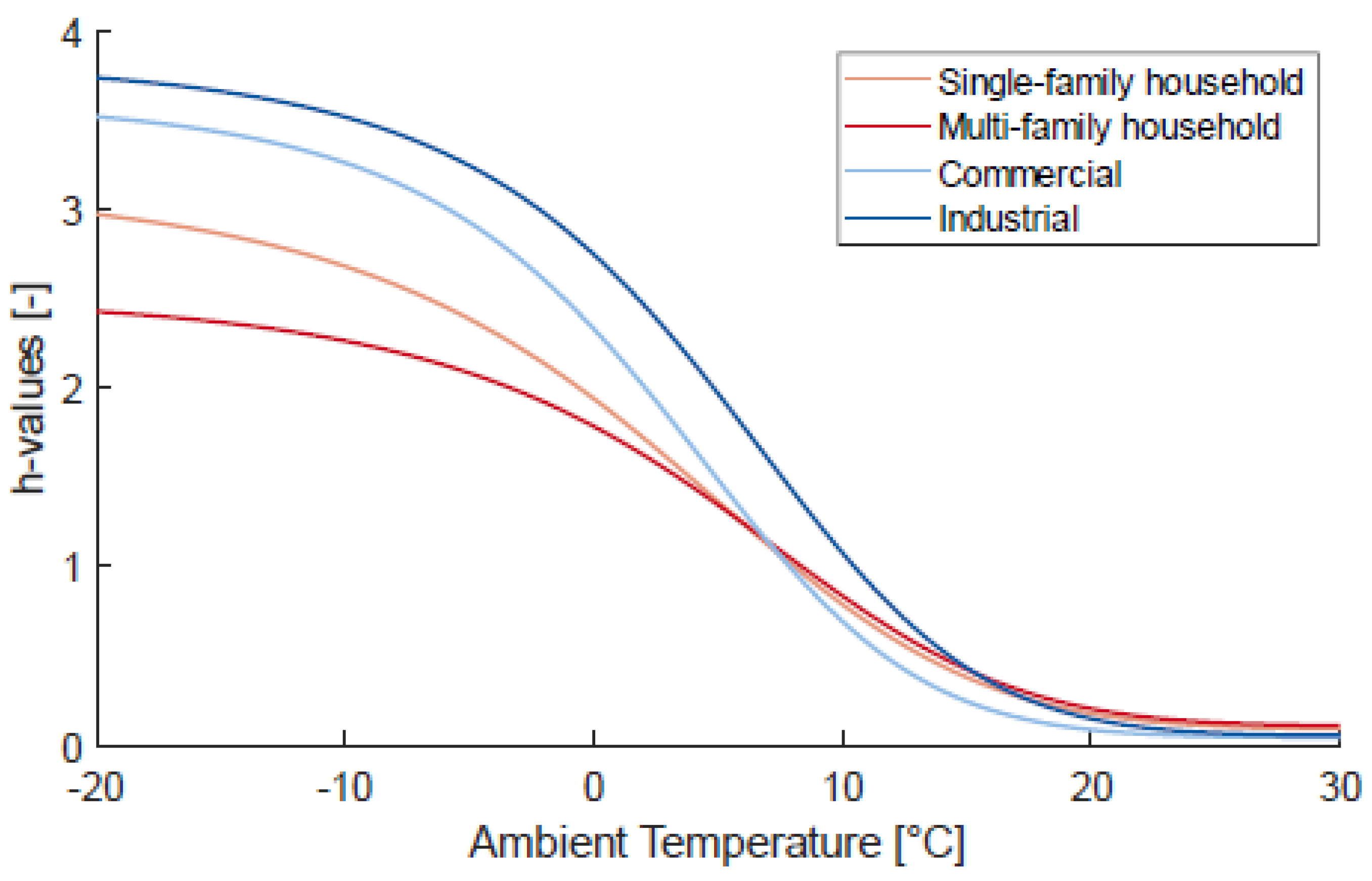
So far, only the information on the annual heat demand is available, but for a detailed analysis and the subsequent dimensioning of the heating grid, a more detailed allocation is desired. The BDEW [38] propose generic heat load profiles as a function of the ambient temperature ϑ = Tamb. Each building type is matched to a sigmoid equation h = f(ϑ) with the building type specific parameters A, B, C, D and ϑ0:
The parameters for the building types of single-family household, multi-family household, commercial, and industrial are listed in Table 2, whose evolution over the ambient temperature are presented in Figure 2. Note that the accommodational buildings have a flatter curve than the commercial buildings and are hence not as sensitive to a change in temperature. It is assumed that the h-values of accommodational buildings do not depend on the day of the week, whereas the commercial buildings have a higher heat demand on weekdays and a lower demand on weekends. The correction factors FWD for the h-values of commercial buildings are listed in Table 3. Since the h-values of accommodational buildings are independent of the day, FWD = 1 is set for each day and building type [38].
Table 2.
Parameters for sigmoid equations for different building types [38].
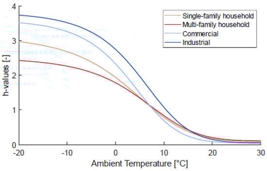
Figure 2.
Sigmoid equations for different building types over ambient temperature.
Table 3.
Daily correction factors FWD for h-values of commercial buildings [38].
The ambient temperature data Tamb for the year 2019 is obtained from the DWD (German Meteorological Service), which provides the data in an hourly resolution [39]. Hence, the hourly heat demand qhourly can be calculated for each of the 8760 h of the year:
qhourly(t) = αh(ϑ(t))FWD(t)
The multiplication factor α is different for each building and is calculated with the annual heat demand qannual, derived from the heat registry Hamburg:
Figure 3 shows the load duration curve for total heat demand in all considered buildings in Wilhelmsburg. The peak load is 64 MW, which corresponds to an ambient temperature of −7.8 °C. The higher the ambient temperature, the lower is the heat demand, whose minimum value is 1.9 MW. Here, the ambient temperature is 35.5 °C. In conclusion, utilizing the building data from OpenStreetMaps, the heat data from the heat registry Hamburg [36], the sigmoid equations from the BDEW [26] and the temperature data from the DWD [37], the hourly heat demand for each of the 4884 considered buildings in Wilhelmsburg is calculated.
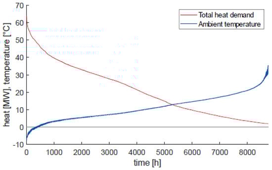
Figure 3.
Heat load duration curve for total heat demand, and corresponding ambient temperature.
2.2. Building Clustering and Grid Improvement
Based on the derived data and the source of the industrial waste heat, the district heating grid is created by clustering the buildings and connecting the obtained allocated nodes. Furthermore, the grid’s efficiency is improved by eliminating nodes, which are too distant from the heat source or have too little heat demand.
To reduce the computational load, the buildings are allocated into clusters, which then represent the buildings’ heat demand. The general idea is to create 15 bins in x-direction and 10 bins in y-direction, resulting to 150 clusters, which are equidistantly distributed. Subsequently, the size of the clusters is adjusted in order to level the heat demand between clusters, i.e., seeking an equal heat demand in each cluster. The clusters with no buildings within are dropped and not considered any further. Hence, the number of clusters is reduced from 150 to 123. Afterwards, the cluster centers are calculated as the heat weighted mean coordinates of the buildings, which are located within the cluster. The calculation is heat weighted, so that the center of the cluster is closer to the buildings with the highest heat demand. Subsequently, the buildings are allocated to the closest cluster center. Hence, the clusters lose their rectangular shape for a polygonal boundary, and buildings change clusters. The center coordinates are not reevaluated.
Figure 4 shows the final clusters with their cluster centers and boundaries. The size of the buildings’ markers correlates with their heat demand, i.e., larger circles mean higher heat demands. The clusters vary in shape and size, and as desired the clusters in denser areas are smaller than the clusters in the outskirts. Each cluster with all its buildings and the center node is transformed into a graph object using the graph function in Matlab, which creates a connection between each pair of buildings. Subsequently, the minspantree function is applied to the graph to find the shortest connection of all buildings, starting from the center node. The length of the connections is saved as the internal pipe length of the cluster.
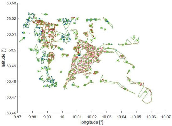
Figure 4.
Clustering of accommodational (red) and commercial (blue) buildings. Centers (x) and boundaries of clusters in green.
The connection of the cluster nodes depends on the root node, i.e., the location where the heat is supplied to the grid. In this model it is assumed that only one heat source is present. Most district heating grids are supplied by a heating plant or a combined heat and power (CHP) plant, which burn fossil fuels to generate heat—and in the case of CHP additionally power. The usage of fossil fuels emits CO2, and it must hence be critically discussed whether that can provide a more sustainable alternative for domestic gas boilers. Alternatively, biomass can be used to power the heating plant, which is then carbon-neutral, but the amount of bioenergy necessary to supply an entire district with heat exceeds any feasible scale. On the other hand, the largest share of Hamburg’s energy-intensive industry is located in the port and is hence close to Wilhelmsburg.
As is common for heating systems, the base load provider is only designed for the base load and not the peak load, because otherwise the system would be oversized for the few moments in which the peak load is demanded. Hence, the 18 MW are an appropriate base load. Furthermore, it is assumed that the temperatures at the root node are constantly 90/60 °C, and the maximum supplied heat power is constant and amounts to 18 MW.
Analogous to the connections in each cluster, the general heating grid is derived by applying Matlab’s minspantree function to the nodes, transformed into a graph object. The 123 nodes are hence connected by 122 connections, because each node needs exactly one connection leading to it. The root node however does not have a connection, because the grid starts there. The initial heating grid is depicted in the upper plot in Figure 4. The nodes are numbered from 1 to 123, beginning in the bottom left corner and ending in the upper right corner. The root node is node 111. Note that the heating grid is finely branched, with long distances to the end nodes, e.g., node 1 in the bottom left corner or node 10 in the bottom right corner. Longer distances evidently result in higher heat losses, which lower the efficiency of the heating grid. It is hence desired to balance the delivered and lost heat. Consequently, the connectivity density rcon,node is calculated as the ratio between the supplied heat Qsup,node and the distance to the node Snode [40]:
The distance to the node Snode is composed of the distance from the root node Sroot,node and the distance of the grid within the cluster Sin,node, multiplied by 2 to account for the return flow. Hence, to discard the least efficient nodes, the nodes with the worst connectivity density are iteratively eliminated from the graph. Afterwards, the minspantree is reevaluated for the new, smaller grid. Thereby, less heat is supplied, but on the other hand, the heat losses are simultaneously reduced. This elimination is continued until the supplied heat falls below 85% of the initially demanded heat.
2.3. Building Location and Heat Demand Data
In the next step, the properties of the heating grid, including especially the diameter of the pipes, are calculated. This determines the heat loss along the edges of the grid, as shown below. Consequently, the lost heat reduces the feed temperature and raises the return temperature. It is still assumed that the first node has the supplied feed and return temperatures of 90 °C and 60 °C.
The cumulated heat flow on each edge in hourly resolution , i.e., the total heat flow on this edge which supplies all subsequent nodes, is the product of the mass flow on the edge , the heat capacity of water cw, and the difference of the feed and the return temperature on this edge Tin,edge and Tout,edge:
It is assumed that the temperatures remain constant on each edge, and are equal to the temperatures of the previous node. Thus, for example, the two edges leading away from the root node have the same temperature as the root node.
The diameter of an edge Dedge is a function of the maximum mass flow on the edge . With a fixed specific pressure loss of R = Δp/l = 300 Pa/m, the flow coefficient λ, the density of water ρw and , Dedge is calculated as [40]:
For high enough Reynold numbers, λ depends on Dedge and the roughness height k, which is set to 0.01 mm [28]:
The two equations for Dedge and λ are iteratively repeated until the relative change in λ is Δλrel < 10−3. The calculation converges after 4 iterations. With Dedge, the specific heat loss coefficient Uedge is calculated. The Planungshandbuch Fernwärme (planning manual district heating) [40] proposes empirical values for Uedge, which are then logarithmically approximated. The heat loss in feed direction and in the return flow are subsequently calculated with the edge length ledge as:
The ambient temperature Tamb is the ground temperature in Wilhelmsburg for the year 2019 at a depth of 1 m [39]. Hence, the flow into a node or from a node loses heat, which can be translated in a lost temperature difference ΔTin,edge and ΔTout,edge:
As before, the edge corresponding to a node is the edge leading to the root node. The node temperatures Tin,node and Tout,node are then calculated as:
The index prev denotes here the previous node connected by the edge, which is assumed to have the same temperature as the edge.
As seen above, the heat loss determines the temperatures, which in return determine the heat loss. Thus, the calculation is started at the root node where the temperatures are set as a boundary, and subsequently the heat loss on the adjacent edges is calculated. The temperatures on the then adjacent nodes are calculated next. This procedure is continued until the end nodes. The problem with this procedure is that the physicality of the solution cannot be guaranteed because the feed and return flows are calculated separately. Hence, at the furthest nodes, the temperatures can change places. The reason for this behavior is that far nodes with relatively little heat demand have a higher heat loss than heat demand, which is not physical. Hence in this project, the nodes’ heat demand is iteratively increased. The new cumulated heat demand is the sum of the previous heat demand and the heat losses which occur in both flows until the node :
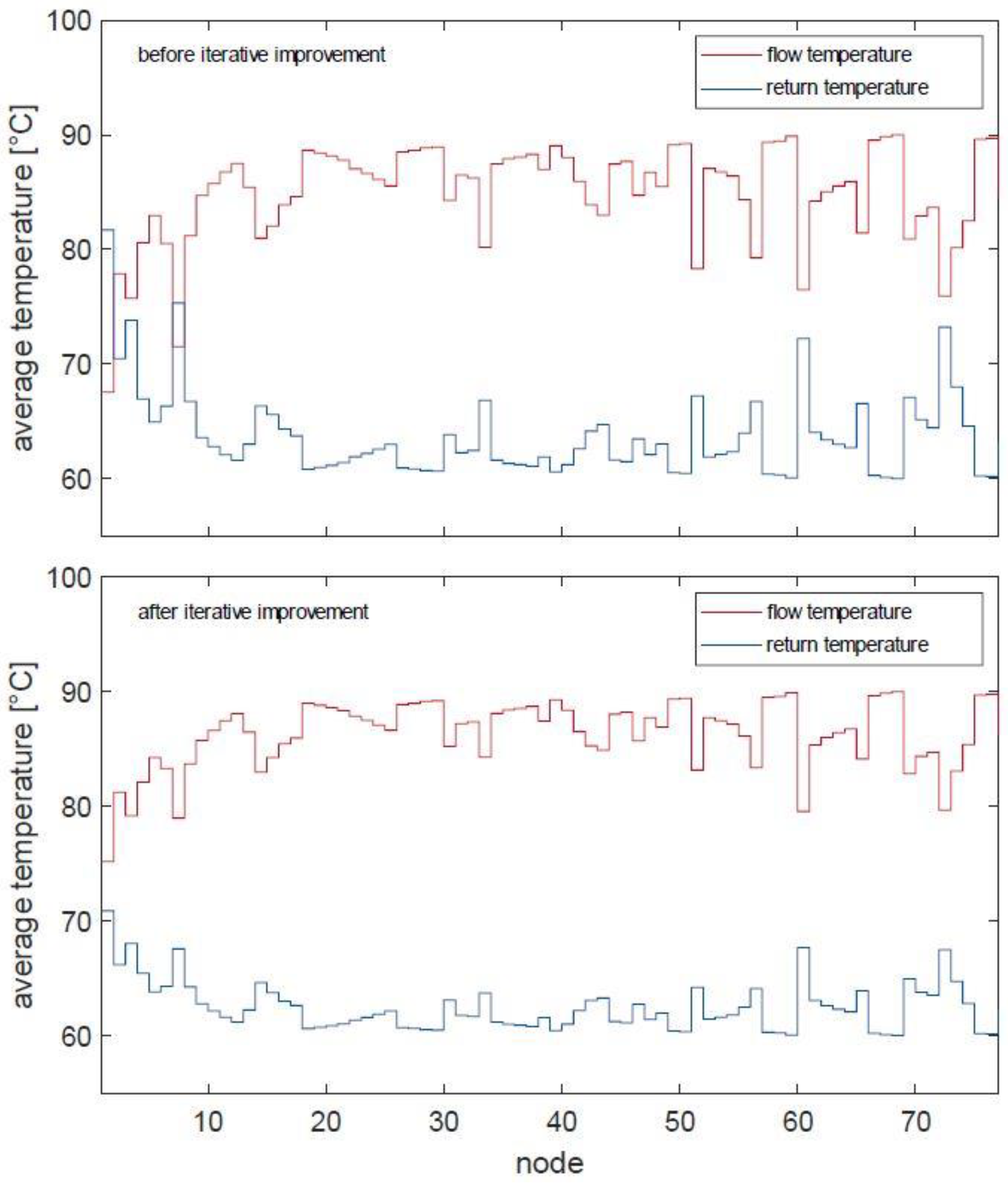
But a higher heat demand leads to a higher mass flow, which leads to a larger diameter, which itself leads to a higher heat loss coefficient. Hence, the heat losses themselves are higher as well. Thus, the recalculation of the heat demand is iteratively repeated until the change in heat demand is lower than 0.1%. The result, which converges after three iterations, can be seen in the bottom plot of Figure 5.
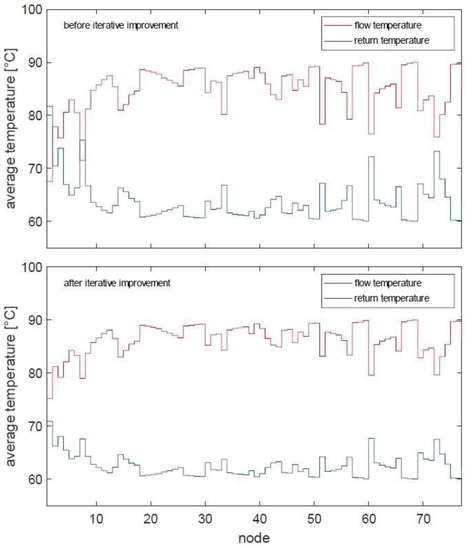
Figure 5.
Mean feed and return temperature of nodes before and after iterative improvement.
2.4. Numerical Model
This chapter described the heating circuit of one building as an example for the reader. The Simulink model is split into three parts: first the calculation of the necessary feed and return temperatures of the heating circuit, second the partial supply of heat by the district heating, and third the peak load boiler.
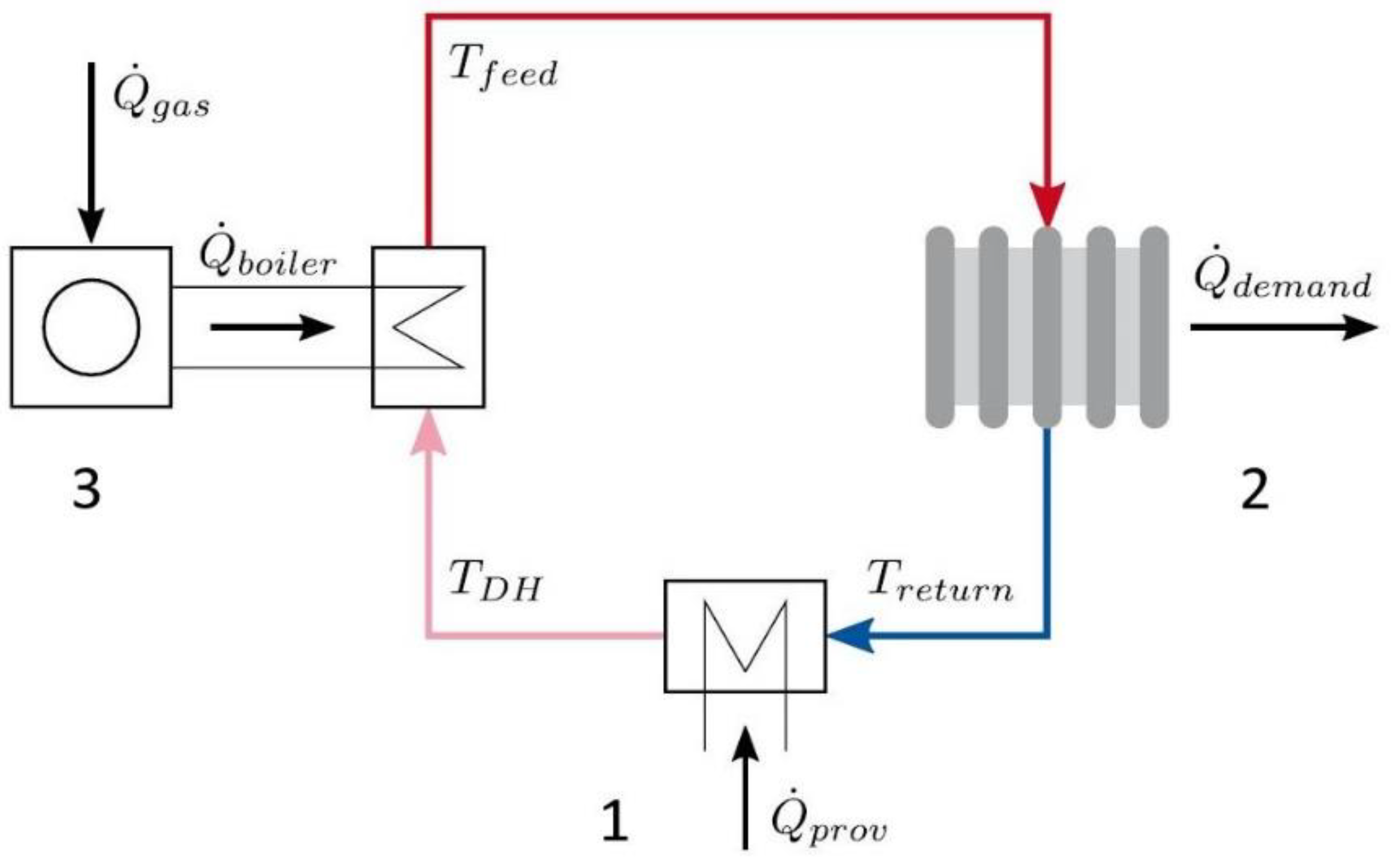
Figure 6 depicts the general structure of the heating in the building. The cold heating water temperature Treturn is increased by the provided heat from the district heating to a medium temperature TDH, which varies dependent on the demanded feed temperature Tfeed and the provided heat. If the district heating can supply the entire heat demand, the boiler is not used and TDH = Tfeed. The peak load boiler then burns gas represented by the chemical power to supply the rest of the demanded heat :

Figure 6.
Schematic heating circuit with district heating and boiler.
First, the heating temperatures Tfeed and Treturn are calculated. Assuming a constant mass flow in the heating circuit , the load ratio mdemand between current demand and nominal, i.e., maximum possible demand is:
The nominal temperatures are Tfeed,0 = 70 °C and Treturn,0 = 55 °C. Derived from the thermodynamic characteristics of radiators, the mean water temperature Tw = 1/2(Tfeed + Treturn) is [41]:
with the room temperature Tl = 20 °C and the exponent n = 1.3. Tfeed and Treturn are then calculated as [41]:
Note that the temperature difference increases for higher loads. Figure 7 shows the Simulink subsystem to calculate the feed and return temperatures. Most of the inputs are constants, whereas is variable and hence passed to the model as a timeseries object through a “From Workspace” block. Subsequently, the provided heat is translated into a temperature difference in the heating circuit with the and (21):
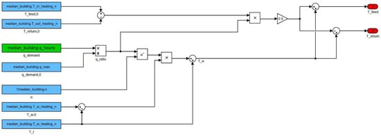
Figure 7.
Simulink subsystem of feed and return temperature calculation. Constants (blue), outputs (red) and From Workspace blocks (green).
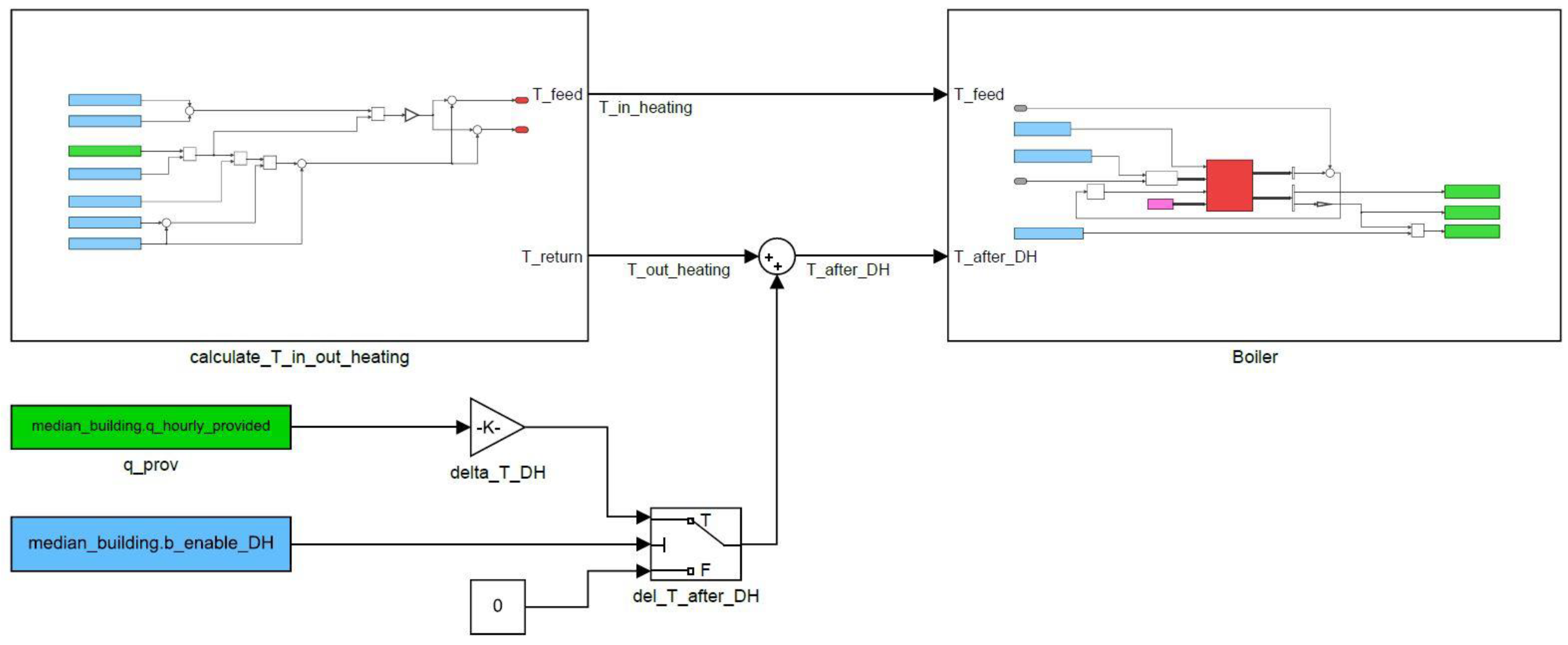
Thus, the temperature after the district heating TDH is calculated, as seen in Figure 8. is variable and hence passed as a timeseries object. The heat transfer from the district heating grid to the domestic heating circuit is not modeled in detail. Furthermore, the Boolean benableDH sets whether the district heating is used in the simulation. To calculate and the boiler efficiency ηboiler, Tfeed and TDH are passed to the subsystem “Boiler”.
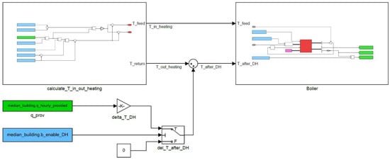
Figure 8.
Simulink connection of the two subsystems calculation of heating temperatures and boiler, and calculation of temperature after district heating. Constants (blue) and From Workspace blocks (green).
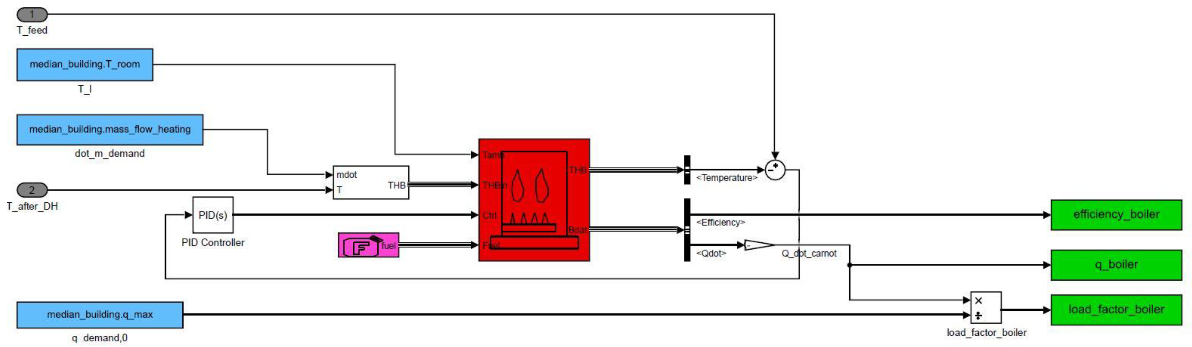
In the subsystem “Boiler” (Figure 9), the toolbox Carnot is used to simulate the boiler operation with the Condensing Boiler block, as seen in Figure 8. Furthermore, a PID controller is used to control Tfeed. The controller manipulates the supplied chemical energy to the boiler. Inherently, the integral behavior of the PID controller ensures no steady-state control error in Tfeed. The fuel block is set to gas, and the water temperature entering the boiler is set to TDH. The efficiency ηboiler, and the load factor βboiler = are passed back to the workspace.
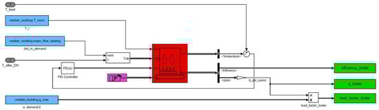
Figure 9.
Simulink subsystem to calculate the boiler power and efficiency. Usage of toolbox Carnot and PID controller. Constants (blue), inputs (grey), Condensing Boiler block (red) and To Workspace blocks (green). The block to calculate THD concatenate the mass flow and temperature information to be passed to the boiler block.
ηboiler is calculated as (22):
The Carnot toolbox works on a seconds-based time scale, and the variable input signals and are therefore interpolated from an hours-based to a seconds-based time scale. Furthermore, a simulation interval of two days is selected where the district heating can sometimes provide the entire heat, and sometimes cannot. Figure 10 shows the results of the two simulated days. The district heating provides the base load, while the boiler provides the peak load. In the afternoon of both days, the district heating covers the entire heat demand, and the boiler is off. The extracted variables ηboiler and βboiler are used to calculate a generic fit of ηboiler as a function of βboiler. Since it is assumed that this characteristic is the same for each building and boiler, the load factor and subsequently the efficiency are calculated for each building.
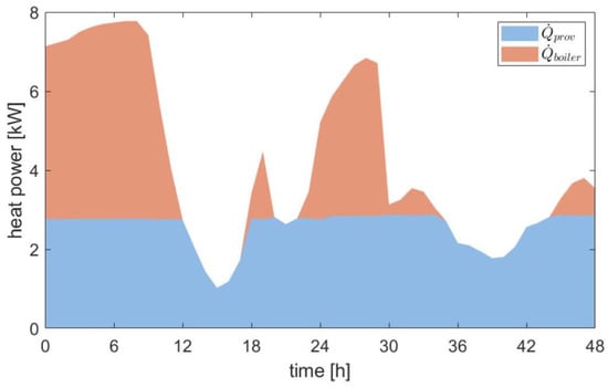
Figure 10.
Power results from simulation of median building, shared supply between district heating (blue) and boiler (orange).
2.5. Building Location and Heat Demand Data
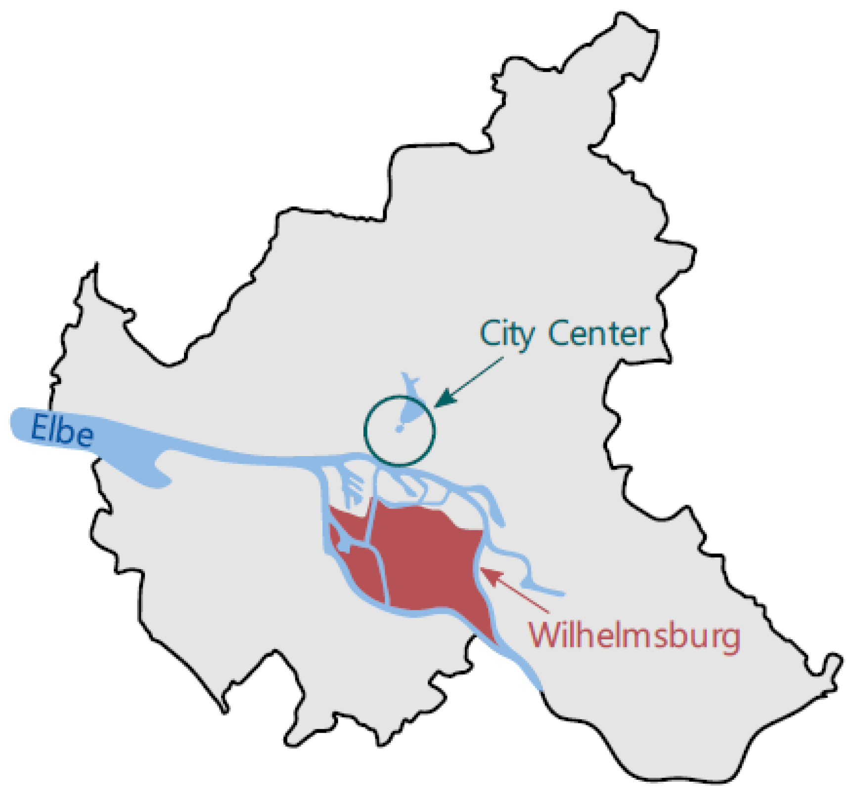
Wilhelmsburg is located south of the northern main river branch on the largest river isle, as depicted in Figure 11. It is Hamburg’s largest district by area (35.4 km2) and its fifth largest district by population (53,519), according to the Statistikamt Nord (census bureau north) [42]. Historically, the southern districts were closely interlinked with the port, the second largest port in Europe. Due to its location close to the port and south of the Elbe, Wilhelmsburg traditionally offered low priced housing and hosted low-income workers who were employed at the port or the adjacent industry. As in all of Germany, after the second World War, many immigrant families came to Hamburg to work in the industry and hence lived predominantly in districts like Wilhelmsburg [43,44].

Figure 11.
Schematic map of Hamburg, the river Elbe and Wilhelmsburg.
Hamburg has a widespread district heating grid, which satisfies circa 22% of the city’s heat demand, and is hence Germany’s second largest district heating grid. As of 1 December 2020, more than 500,000 households are connected to the heating grid [45]. Though, this heating grid is only placed north of the Elbe, i.e., in the districts adjacent to the city center. Wilhelmsburg is not part of this heating grid, even though it is close to the heating plants supplying the grid.
3. Results
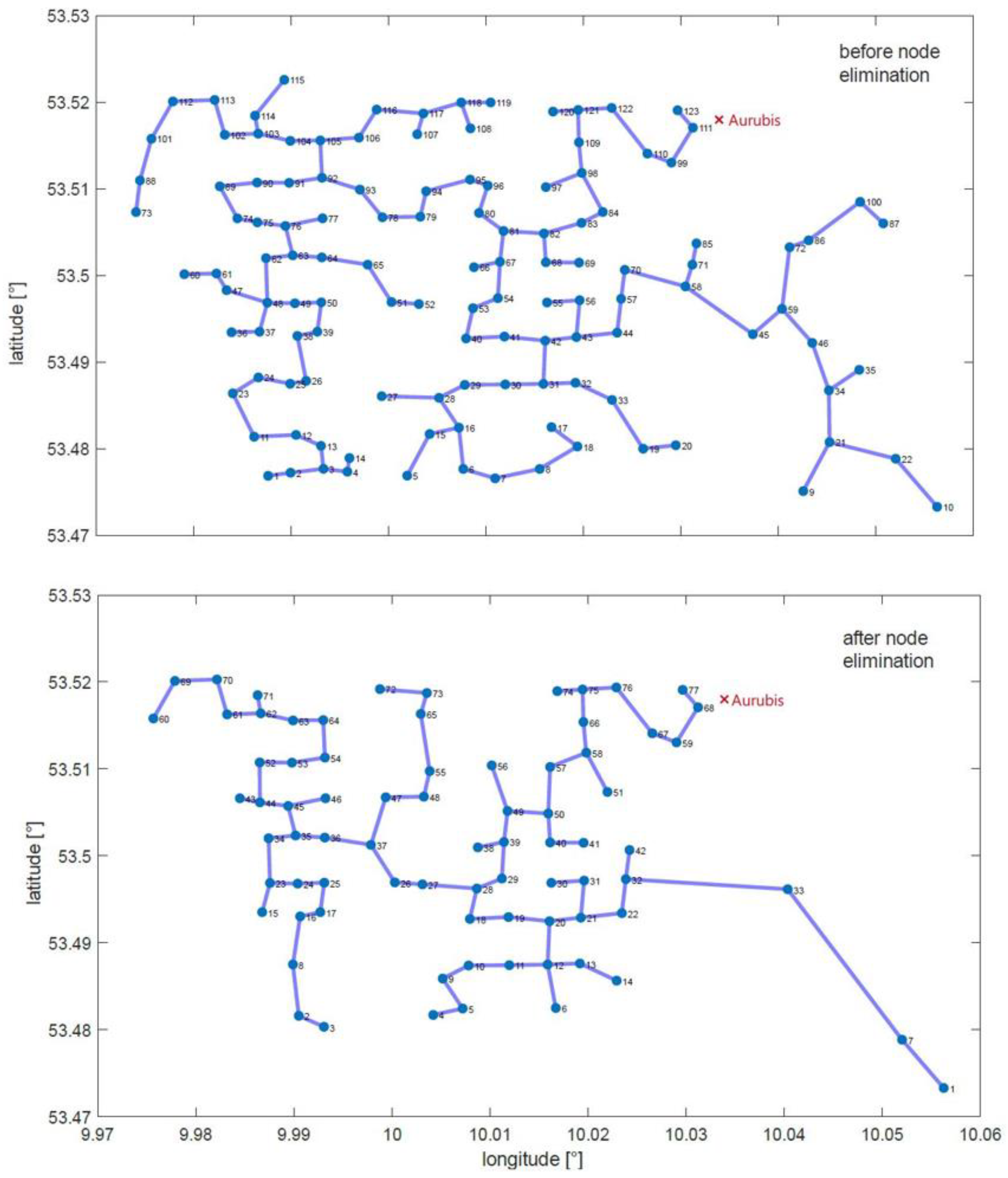
The goal of district heating is to substitute the usage of conventional heating partially or entirely, which are mainly domestic gas boilers in each building. Hence, the previous results of the district heating grid are used to calculate the saved gas in Wilhelmsburg. The boiler efficiency is derived by implementing the district heating connection and the boiler in Simulink for the median building of the district. Afterwards, the calculated efficiency characteristics are applied to all buildings to calculate the saved gas. Figure 12 depicts the elimination of nodes, beginning with the upper plot with the initial nodes, to the lower plot, where the remaining 77 nodes after the elimination are shown. Note that the nodes and connections close to the root node remain the same, since their distance to the root node is small and thus their connectivity density is high.
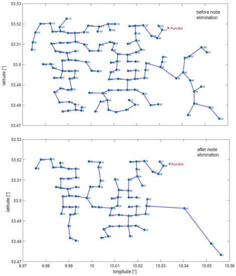
Figure 12.
District heating grid with nodes and connection before (top) and after (bottom) node elimination. Reduction from 123 to 77 nodes.
Figure 13 shows the resulting heat demand at each node and hence the necessary heat flow along the connections of the heating grid. The heat is supplied at the root node 68 and distributed across the grid to each node. In summary, by allocating the buildings to clusters, the computational load can be reduced. Hence, the 4884 buildings are condensed to 123 clusters, which then incorporate the heat demand of the buildings in each cluster. The clusters are connected to a heating grid by utilizing the graph theory functions in Matlab, especially minspantree, to calculate the shortest connection between the nodes. Furthermore, to increase the overall connectivity density and hence efficiency of the heating grid, the 46 nodes with the lowest connectivity density are eliminated from the grid.
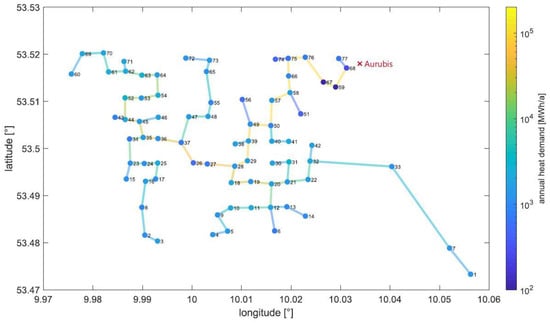
Figure 13.
Annual heat demand in district heating grid at each node and connection (logarithmic scale).
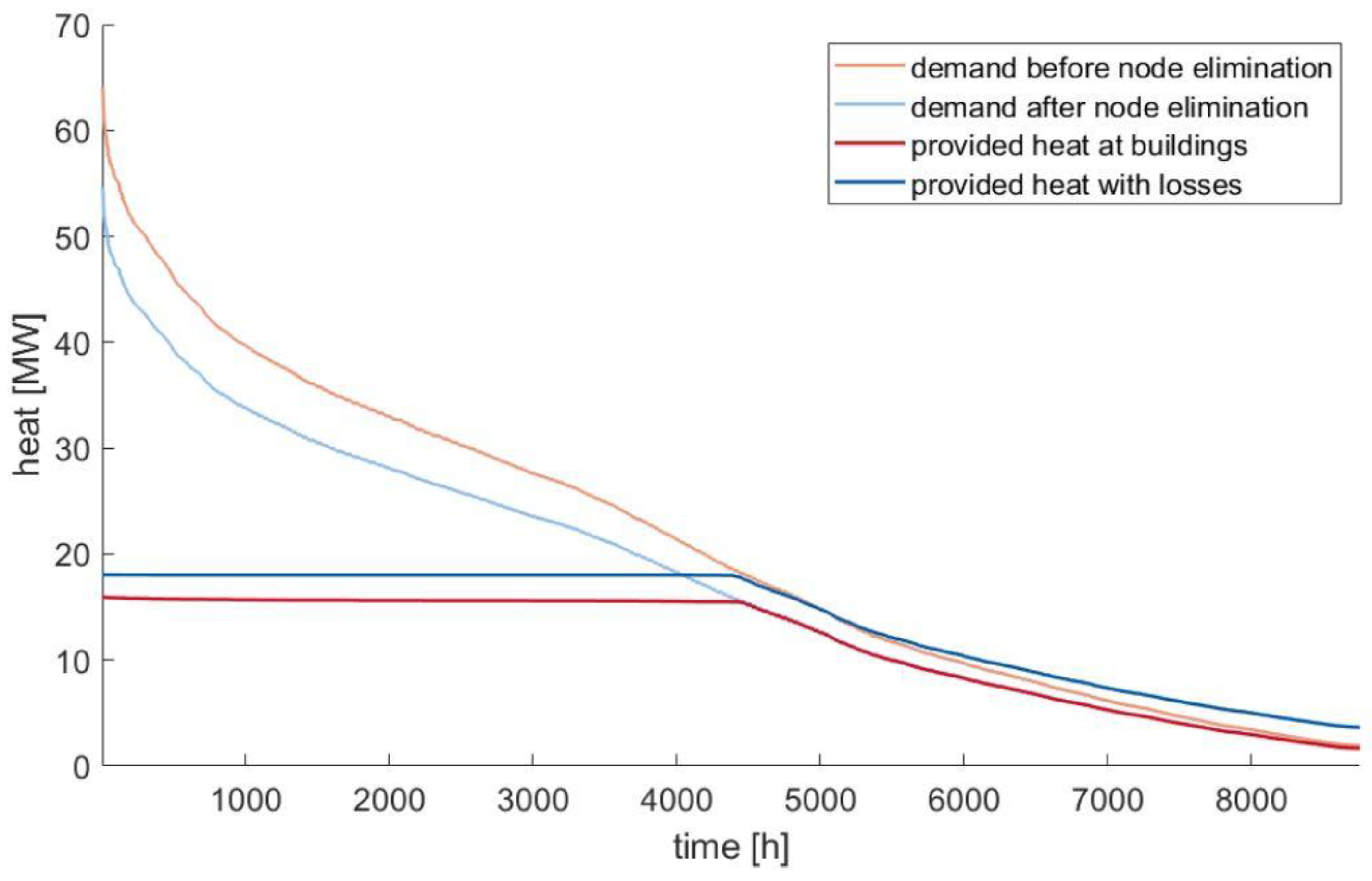
All feed temperatures are higher than the return temperatures, even though the furthest nodes still have the lowest temperature difference. In practice, the temperature difference at node 1 might be too small to be technically feasible, which is neglected in this article. Figure 14 depicts the load duration curves of the heat demand before node elimination (compare Figure 3), the heat demand after node elimination, the provided heat at the buildings , and the provided heat with losses, which is equivalent to the effectively supplied heat from the energy provider at the root node . There is an almost constant offset of roughly 2.5 MW between and , which indicates the overall heat loss. This results in an average efficiency of the district heating grid ηgrid of (23):
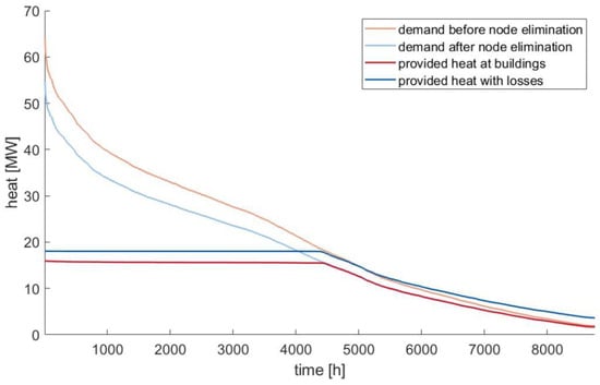
Figure 14.
Load duration curves of heat demand before node elimination (orange), heat demand after node elimination (light blue), provided heat at buildings (red) and provided heat with losses (blue).
Thus, the overall relative heat loss amounts to ΔQloss,rel = 16.46%, which is undistinguishably similar to the benchmark of ΔQloss,rel,bm = 16.5% of a real district heating grid presented by the Planungshandbuch Fernwärme [40]. Aurubis provides a maximum heat power of 18 MW and an annual amount of energy of 120 GWh [46]. Applying the same maximum heat power to the model in this article as seen in Figure 14, the provided annual energy amounts to 119.63 GWh. That shows that the assumptions made in this project hold and thus the model represents the behavior of real heating grids well. In summary, in this project a district heating grid is developed based on openly accessible data for the buildings in Wilhelmsburg and their heat demand, which are then allocated in clusters. Subsequently, the clusters are connected to a heating grid starting from the root node. In the last step, the least efficient nodes are eliminated and the heat loss along the edges is calculated. The heat loss is then iteratively added to the supplied heat.
As seen in Figure 14, the supplied heat is lower than the overall heat demand, first due to the elimination of nodes in the grid and second due to the maximum heat power of 18 MW. The remaining heat is thus still supplied by domestic gas boilers, which are then used as peak load boilers. Hence, the cold heating water is first heated by the district heating and then—if necessary—heated further by the boiler to the desired feed temperature. It is assumed that each building shows the same boiler properties, i.e., the boiler efficiency characteristics are the same for every building. Thus, a single building is selected, and the boiler efficiency is calculated. To select a building which shows an appropriate characteristic, the median heat demand of all accommodational buildings is selected and matched to its building. Then, the building’s heat demand and the provided heat are extracted and fed into the Simulink model.
The amount of consumed gas is characterized by the consumed chemical energy Qgas = Qboiler⁄ηboiler(βboiler). With the previous calculations, the chemical energy is derived for each building and summed up for all 4884 buildings. Due to the different load factors—and hence efficiencies—for when the district heating is used and when it is not, Qgas is evaluated for both cases Qgas,noDH and Qgas,DH. The entire consumption is Qdemand = 182.59 GWh, while the provided heat by the district heating grid is Qprov = 99.91 GWh. Without district heating the consumed amount of gas is Qgas,noDH = 186.49 GWh, while this is reduced to Qgas,DH = 89.17 GWh when the district heating is used. Hence, by utilizing the district heating, a total amount of gas of ΔQgas = 97.32 GWh per year is saved. The Bundesnetzagentur (Federal Network Agency of Germany) lists an average domestic gas price in Hamburg for the year 2019 of kgas = 0.0599 €/kWh [47]. The CO2 emissions of domestic gas are egas = 0.2012 kgCO2/kWh according to the Umweltbundesamt (German Environment Agency) [48,49]. Hence, by saving ΔQgas = 97.32 GWh of gas annually, CO2 emissions of ΔmCO2 = 19,585 tCO2 are avoided, and the customers save ΔKgas = €5.83 mil annually. In the existing project by Aurubis and Enercity, the benchmark use of the district heating grid avoids ΔmCO2,bm = 20,000 tCO2 annually [46]. As before, the model presented in this article tracks the benchmark project well in terms of CO2 avoidance.
In summary, the simulation of the heating circuit in an exemplary median building yields the boiler efficiency as a function of the boiler’s load, which is then used to calculate the saved gas of every building. The usage of the district heating grid saves ΔQgas = 97.32 GWh annually, which results in financial savings of ΔKgas = €5.83 mil and avoided CO2 emissions of ΔmCO2 = 19,585 tCO2.
4. Discussions and Conclusions
In this paper, a different approach is presented to plan a district heating grid based on the optimization of building clusters with the aim of improving the nodes of the grid. GIS technology was also employed to collect and group data of the buildings, from geometrical to heat demand. In the literature, few works described in detail those approaches, therefore this research wants to fill this gap. A case study is chosen to validate the method proposed, in the district of Hamburg city, Wilhelmsburg. The scope is to connect this district with the existing thermal network of the city. Moreover, this approach investigates the usage of industrial waste heat as the grid’s heat source, which is CO2-neutral. Most of Hamburg’s energy-intensive and high-temperature industry is located at the port, which spans across the islands in the river. To simulate the model, Matlab/Simulink is used. After the data collection, the district heating grid is created by clustering the buildings and connecting the obtained nodes. A single building is modelled to investigate the benefit in terms of energy saving due to the replacement of gas boilers with DH systems. As a result, the usage of the district heating grid saves 97.32 GWh annually, which provides financial savings of €5.83 million, and avoided CO2 emissions of 19,585 tCO2. Last but not least, the proposed method allows other designers and practitioners to adapt it to different urban settlements; this issue is also the core of this research. Future developments will be involved for the investigation of the substations of the buildings connected to the grid, being an essential key for the economic and environmental assessment of users.
Author Contributions
Conceptualization, L.P., J.M., F.N.; methodology, J.M.; software, J.M.; validation, L.P., F.N.; data curation, L.M.P.; writing—original draft preparation L.P., J.M., F.N.; writing—review and editing L.P., J.M., F.N.; visualization, L.P., F.N.; supervision L.d.S.; funding acquisition L.M.P. All authors have read and agreed to the published version of the manuscript.
Funding
The research activities leading to this study have been partially supported by the project “Progetti per Avvio alla Ricerca” n. AR12117A8A8E6664 funded by Sapienza University of Rome.
Conflicts of Interest
The authors declare no conflict of interest.
Nomenclature
| q | annual heat demand [kWh/yr] | e | Emission factor [kgCO2/kWh] |
| A | Area [m2] | K | Gas expenditure [€] |
| ϑ | Temperature [°C] | Subscripts | |
| F | Correction factor [-] | spec | specific |
| Q | Heat Power [MW] | abs | absolute |
| r | connectivity density [] | acc | accommodational buildings |
| Heat flow [kW/m2] | tot | total | |
| c | Heat capacity [kWh/kg K] | com | commercial buildings |
| Mass flow [kg/s] | amb | ambient | |
| D | Diameter [m] | w | water |
| R | specific pressure loss [Pa/m] | prov | provided |
| λ | flow coefficient [-] | Abbreviations | |
| ρ | Density [kg/m3] | GIS | Geographic information systems |
| k | roughness height [mm] | DH | District Heating |
| U | specific heat loss coefficient [W/m K] | DWD | German Meteorological Service |
| β | load factor [-] | CHP | Combined Heat and Power |
| η | Efficiency [-] |
References
- Eurostat. Sustainable Development in the European Union—Monitoring Report on Progress towards the SDGs in an EU Context, 2017th ed.; Publications Office of the European Union: Luxembourg, 2017. [Google Scholar]
- Battaglia, N.; Massarotti, L.; Vanoli, L. Urban regeneration plans: Bridging the gap between planning and design energy districts. Energy 2022, 254, 124239. [Google Scholar] [CrossRef]
- Nardecchia, F.; Minniti, S.; Bisegna, F.; Gugliermetti, L.; Puglisi, G. An alternative tool for the energy evaluation and the management of thermal networks: The exergy analysis. In Proceedings of the EEEIC 2016—International Conference on Environment and Electrical Engineering, Florence, Italy, 7–10 June 2016; p. 7555645. [Google Scholar]
- Delmastro, C.; Mutani, G.; Schranz, L. The evaluation of buildings energy consumption and the optimization of district heating networks: A GIS-based model. Int. J. Energy Environ. Eng. 2016, 7, 343–351. [Google Scholar] [CrossRef] [Green Version]
- Lavagno, E. Advanced Local Energy Planning (ALEP): A Guidebook; International Energy Agency: Paris, France, 2000. [Google Scholar]
- Pompei, L.; Blaso, L.; Fumagalli, S.; Bisegna, F. The impact of key parameters on the energy requirements for artificial lighting in Italian buildings based on standard EN 15193-1:2017. Energy Build. 2022, 263, 112025. [Google Scholar] [CrossRef]
- Mattoni, B.; Mangione, A.; Pompei, L.; Bisegna, F.; Iatauro, D.; Spinelli, F.; Zinzi, M.; Casaccia, E.C.R. An alternative method for the assessment of the typical lighting energy numeric indicator for different outdoor illuminance conditions. Build. Simul. Conf. Proc. 2019, 2, 1224–1230. [Google Scholar]
- Nardecchia, F.; Pompei, L.; Bisegna, F. Environmental parameters assessment of a new diffuser for air cooling/heating system: Measurements and numerical validation. Build. Simul. 2022, 15, 1111–1132. [Google Scholar] [CrossRef]
- Pastore, L.M.; Sforzini, M.; Lo Basso, G.; de Santoli, L. H2NG environmental-energy-economic effects in hybrid energy systems for building refurbishment in future National Power to Gas scenarios. Int. J. Hydrogen Energy 2022, 47, 11289–11301. [Google Scholar] [CrossRef]
- Pastore, L.M.; Lo Basso, G.; Sforzini, M.; de Santoli, L. Technical, economic and environmental issues related to electrolysers capacity targets according to the Italian Hydrogen Strategy: A critical analysis. Renew. Sustain. Energy Rev. 2022, 166, 112685. [Google Scholar] [CrossRef]
- Pastore, L.M.; Lo Basso, G.; de Santoli, L. Can the renewable energy share increase in electricity and gas grids takes out the competitiveness of gas-driven CHP plants for distributed generation? Energy 2022, 256, 124659. [Google Scholar] [CrossRef]
- Vesterlund, M.; Dahl, J. A method for the simulation and optimization of district heating systems with meshed networks. Energy Convers. Manag. 2015, 89, 555–567. [Google Scholar] [CrossRef]
- Asdrubali, F.; Guattari, C.; Roncone, M.; Baldinelli, G.; Gul, E.; Piselli, C.; Pisello, A.L.; Presciutti, A.; Bianchi, F.; Pompei, L.; et al. A Round Robin Test on the dynamic simulation and the LEED protocol evaluation of a green building. Sustain. Cities Soc. 2022, 78, 103654. [Google Scholar] [CrossRef]
- Sakawa, M.; Kato, K.; Ushiro, S. Operational planning of district heating and cooling plants through genetic algorithms for mixed 0–1 linear program-ming. Eur. J. Oper. Res. 2002, 137, 677–687. [Google Scholar] [CrossRef]
- Weber, C.; Maréchal, F.; Favrat, D. Design and optimization of district energy systems. In Proceedings of the 10th International Symposiumon District Heating and Cooling, Reykjavik, Iceland, 3–5 September 2006; Valentin, P., Serban, A.P., Eds.; Elsevier: Hanover, Germany, 2007; pp. 1127–1132. [Google Scholar]
- Pompei, L.; Nardecchia, F.; Mattoni, B.; Gugliermetti, L.; Bisegna, F. Combining the exergy and energy analysis for the assessment of district heating powered by renewable sources. In Proceedings of the 2019 IEEE International Conference on Environment and Electrical Engineering and 2019 IEEE Industrial and Commercial Power Systems Europe, EEEIC/I and CPS Europe, Genova, Italy, 11–14 June 2019; p. 8783426. [Google Scholar]
- Salata, F.; Golasi, I.; Ciancio, V.; Rosso, F. Dressed for the season: Clothing and outdoor thermal comfort in the Mediterranean population. Build. Environ. 2018, 146, 50–63. [Google Scholar] [CrossRef]
- Salata, F.; Golasi, I.; Verrusio, W.; de Lieto Vollaro, E.; Cacciafesta, M.; de Lieto Vollaro, A. On the necessities to analyse the thermohygrometric perception in aged people. A review about indoor thermal comfort, health and energetic aspects and a perspective for future studies. Sustain. Cities Soc. 2018, 41, 469–480. [Google Scholar] [CrossRef]
- Wang, H.; Yin, W.; Abdollahi, E.; Lahdelma, R.; Jiao, W. Modelling and optimization of CHP based district heating system with renewable energy production and energy storage. Appl. Energy 2015, 159, 401–421. [Google Scholar] [CrossRef]
- Gadd, H.; Werner, S. Achieving low return temperatures from district heating substations. Appl. Energy 2014, 136, 59–67. [Google Scholar] [CrossRef] [Green Version]
- Sciacovelli, A.; Guelpa, E.; Verda, V. Pumping cost minimization in an existing district heating network. In Proceedings of the ASME 2013 International Mechanical Engineering Congress and Exposition, San Diego, CA, USA, 15–21 November 2013; American Society of Mechanical Engineers: New York, NY, USA, 2013; p. V06AT07A066. [Google Scholar]
- Caputo, P.; Costa, G.; Ferrari, S. A supporting method for defining energy strategies in the building sector at urban scale. Energy Policy 2013, 55, 261–270. [Google Scholar] [CrossRef]
- Galante, A.; Torri, M. A methodology for the energy performance classification of residential building stock on an urban scale. Energy Build. 2012, 48, 211–219. [Google Scholar]
- Söderman, J. Optimisation of structure and operation of district cooling networks in urban regions. Appl. Therm. Eng. 2007, 27, 2665–2676. [Google Scholar] [CrossRef]
- Larsen, H. A comparison of aggregated models for simulation and operational optimisation of district heating networks. Energy Convers. Manag. 2004, 45, 1119–1139. [Google Scholar] [CrossRef]
- Larsen, H. Aggregated dynamic simulation model of district heating networks. Energy Convers. Manag. 2002, 43, 995–1019. [Google Scholar] [CrossRef]
- Guelpa, E.; Deputato, S.; Verda, V. Thermal request optimization in district heating networks using a clustering approach. Appl. Energy 2018, 228, 608–617. [Google Scholar] [CrossRef]
- Barbieri, E.S.; Dai, Y.J.; Morini, M.; Pinelli, M.; Spina, P.R.; Sun, P.; Wang, R.Z. Optimal sizing of a multi-source energy plant for power heat and cooling generation. Appl. Therm. Eng. 2014, 71, 736–750. [Google Scholar] [CrossRef]
- Åberg, M.; Widén, J. Development, validation and application of a fixed district heating model tructure that requires small amounts of input data. Energy Convers. Manag. 2013, 75, 74–85. [Google Scholar] [CrossRef]
- Chinese, D.; Meneghetti, A. Optimisation models for decision support in the development of biomass-based industrial district-heating networks in Italy. Appl. Energy 2005, 82, 228–254. [Google Scholar] [CrossRef]
- Burer, M.; Tanaka, K.; Favrat, D.; Yamada, K. Multi-criteria optimization of a district cogeneration plant integrating a solid oxide fuel cell–gas turbine combined cycle, heat pumps and chillers. Energy 2003, 28, 497–518. [Google Scholar] [CrossRef]
- Fabrizio, E.; Corrado, V.; Filippi, M. A model to design and optimize multienergy systems in buildings at the design concept stage. Renew. Energy 2010, 35, 644–665. [Google Scholar] [CrossRef]
- Sontag, R.; Lange, A. Cost effectiveness of decentralized energy supply system taking solar and wind utilization plants into account. Renew. Energy 2003, 28, 1865–1880. [Google Scholar] [CrossRef]
- Trillat-Berdal, V.; Souyri, B.; Fraisse, G. Experimental study of ground-coupled heat pump combined with thermal solar collectors. Energy Build. 2006, 38, 1477–1484. [Google Scholar] [CrossRef]
- Lee, K.H.; Lee, D.W.; Baek, N.C.; Kwon, H.M.; Lee, C.J. Preliminary determination of optimal size for renewable energy resources in building using RETScreen. Energy 2012, 47, 83–96. [Google Scholar] [CrossRef]
- Available online: openstreetmap.org (accessed on 17 December 2020).
- Behörde für Umwelt, Klima, Energie und Agrarwirtsc. Wärmekataster für die Freie und Hansestadt Hamburg. Available online: https://www.hamburg.de/energiewende/waermekataster/8342506/waermekataster-fuer-die-fhh/ (accessed on 17 December 2020).
- GEODE—Groupement Européen des entreprises et Organismes de Distribution d’Énergie; EWIV. Bundesverband der Energie- und Wasserwirtschaft e. V., V. k; Abwicklung von Standardlastprofilen Gas: Berlin, Germany, 2018. [Google Scholar]
- Deutscher Wetterdienst. Climate Data Center Suche. Available online: https://cdc.dwd.de/portal/202007291339/searchview (accessed on 17 December 2020).
- Arbeitsgemeinschaft QM Fernwärme. Planungshandbuch Fernwärme; EnergieSchweiz: Bern, Switzerland, 2017. [Google Scholar]
- Lucas, U.-P.K. Vorlesung Energiesystemtechnik Vorlesungsumdruck; Lehrstuhl für Technische Thermodynamik: Aachen, Germany, 2013. [Google Scholar]
- Statistikamt Nord. Hamburger Stadtteil-Profile Berichtsjahr 2019; Statistikamt Nord: Hamburg, Germany, 2019. [Google Scholar]
- Statistikamt Nord. Hamburger Stadtteil-Profile 2016; Statistikamt Nord: Hamburg, Germany, 2016. [Google Scholar]
- Bezirksamt Hamburg-Mitte. Sozialraumbeschreibung Wilhelmsburg; Bezirksamt Hamburg-Mitte: Hamburg, Germany, 2015. [Google Scholar]
- Beckereit, M. Anschluss der 500.000. Wohneinheit; Wärme Hamburg: Hamburg, Germany, 2020. [Google Scholar]
- Aurubis and Enercity. Industriewärme—Ein Klimabündnis von Aurubis und Enercity; Aurubis and Enercity: Hamburg, Germany, 2018. [Google Scholar]
- Bundesnetzagentur. Verbraucher-Kennzahlen Monitorbericht 2019; Bundesnetzagentur: Bonn, Germany, 2019. [Google Scholar]
- Umweltbundesamt. CO2-Emissionsfaktoren für Fossile Brennstoffe; Umweltbundesamt: Dessau-Roßlau, Germany, 2016. [Google Scholar]
- Umweltbundesamt. Grenzwerte für Schadstoffemissionen von PKW; Umweltbundesamt: Dessau-Roßlau, Germany, 2016. [Google Scholar]


Publisher’s Note: MDPI stays neutral with regard to jurisdictional claims in published maps and institutional affiliations. |
© 2022 by the authors. Licensee MDPI, Basel, Switzerland. This article is an open access article distributed under the terms and conditions of the Creative Commons Attribution (CC BY) license (https://creativecommons.org/licenses/by/4.0/).