Abstract
The paper aims to capitalize on the new features that are offered by the Microsoft Excel calculation program for reliability modeling, using the Median Ranks estimator that is calculated directly with the BETA.INV function, not estimated by various algebraic estimators, as is generally the case. Starting from this first step, a method of modeling reliability is elaborated through the three-parametric Weibull model that is based exclusively on this software, which is accessible to anyone and can be used even in the case of online learning, which is widespread in recent years due to the pandemic situation. The probability plotting method is applied, using the Median Ranks estimator that is calculated directly with the BETA.INV function for a probability equal to 0.5. A flowchart is made for the proposed method, which could be easily translated into a calculation program. By representing in logarithmic coordinates, we determined the Weibull models for different values that were initially adopted for the location parameter: using as a criterion the coefficient of determination that was obtained using the trendline function for the linear model, it was possible to identify, by successive tests, the optimal value of the location parameter—for which the three-parametric model has a good likelihood. By the proposed method, this value can be found following this iterative process. So, based on the current facilities of the Microsoft Excel program, a precise and easy-to-apply method has been achieved, through which an appropriate three-parametric Weibull model can be identified.
1. Introduction
The three-parametric Weibull model is considered the most suitable for reliability modeling, but its identification requires laborious methods, which is why the bi-parametric Weibull model is frequently used [1]. Thus, only bi-parametric Weibull models can be identified in general [2,3,4]—even in the case of dedicated software such as Weibull++ [5,6], and operating software allows computation with only bi-parametric Weibull models, such as Windows Microsoft Excel in Microsoft Office package [7].
But in recent years the usual MS Office computing programs have been supplemented with new features, including mathematical functions such as the BETA.INV function, which was introduced in 2010 [8], which allows the development of methods for identifying a three-parametric Weibull model.
Since conducting reliability studies through common computer packages, accessible to all, is very important (including in the case of online education, widespread in recent years due to the pandemic situation), this paper aims to capitalize on these opportunities that are offered since 2010 by Microsoft Excel [9,10] to develop a method for identifying the three-parametric Weibull model. Thus, along with the two parameters of the bi-parametric Weibull model (the shape parameter and the scale parameter), the objective of the paper can be expressed even more concretely: based on the actual Microsoft Excel program, to identify a method by which the third parameter can be identified—the location parameter—and, thus the three-parametric Weibull model.
Various methods can be used to obtain the appropriate mathematical model for the analytical description of a data distribution [11,12,13]: analytical methods—the least square method (LSM), the maximum likelihood method (MLM) and the method of moments (MOM), [14,15]—or graphical representation.
The most appropriate way to develop a method for identifying the three-parametric Weibull model based on the Microsoft Excel utility is the graphical path, because this utility contains the linear regression function through which the Weibull function can be linearized. Thus, using as a variable the failure times we can identify the bi-parametric Weibull model (for which the location parameter is equal to zero), but we can do more than that: using as a variable the failure times adjusted with the location parameter (a non-zero value), a three-parametric model is obtained. As a result, research is being developed in this direction, which will be presented below.
Thus, the main steps that will be taken are:
- Estimating the function of distribution of failure times using the BETA.INV function;
- Identification of the bi-parametric Weibull model by the known method of linear regression;
- Identification of the optimal location parameter—for which the resulting three-parametric Weibull model has the maximum coefficient of determination R;
- Argumentation the efficiency of the proposed method, based exclusively on the facilities of the Microsoft Excel program, by the superior likelihood of the three-parametric Weibull model that are obtained compared to the bi-parametric model.
2. Methods and Results
2.1. The Three-Parametric Weibull Model Parameters
The three-parametric Weibull model is defined by the following expression for the reliability function or the survival function [16]:
or by the function of unreliability, also called function of distribution of the time of good operation:
where:
- -
- γ—location parameter or position parameter, this being a constant value that defines when the variation of the survival function R(t) starts.
- -
- η—scale parameter, which characterizes the extent of the distribution on the time axis. So, in the particular case when (t − γ) is equal to η, this parameter can be highlighted; because R(t) calculated with the relation (1) will be:
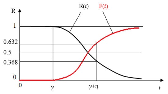
Figure 1.
Highlighting parameters γ and η of the three-parametric Weibull model on the graphs R(t) and F(t).
- -
- β—shape parameter, is dimensionless and is the parameter that determines the variation of the variation curves for the reliability indicators.
2.2. Choosing the Optimal Estimator for the Distribution Function F(t)
Obviously, when the Weibull mathematical model for product reliability is known, the previous analytical relationships are used. But when the model is not known, obtaining it requires the calculation of one of the reliability indicators through the statistical processing of the values for failure times, and then, the modeling of the distribution of these singular values through a continuous mathematical function as appropriate as possible.
Due to its cumulative character, the most frequently used indicator for modeling reliability is the unreliability function or the distribution function F(t), which expresses the probability that the product will fail at the time t.
Having a set of values in ascending order with the values of time and at which the n products failed, the values F(ti) can be estimated with various computational relationships.
Dedicated calculation programs for reliability analysis generally have two estimators for the distribution function: the Median Ranks estimator and the Kaplan–Meyer estimator, usually the default one being the Median Ranks estimator [17,18], which leads to the most probable results.
The Median Ranks method consists of estimating the unreliability for each failure time by determining the median rank for each failure.
Thus, the median rank MRi is the value of the probability of failure of i products out of the total of n products, F(ti), for which the time ti represents the quintile of 50%. That is, MRi estimate for F(ti) represents the value for which at that moment ti the probability that the true value is higher than F(ti) is equal to the probability that the true value is lower than F(ti)—therefore equal to 0.5.
The F(ti) values result, according to the binomial law (Bernoulli), from the relation:
With the help of a special dedicated computing program, such as Reliasoft Weibul++, MR can be determined (so we can estimate F(ti) for any order number i, from 1 to n).
In the absence of a calculation program that allows the calculation of the Median Ranks estimator, it can be approximated by various algebraic estimators, whose calculation is simple in Microsoft Excel, as follows:
- -
- the Herd–Johnson estimator, used in 1960–1964, but also proposed by Weibull in 1939 [4]:
- -
- the Hazen estimator (2014):
- -
- the Benard estimator (1953):
- -
- the Blom estimator (1958) [20]:
These estimators of the F(t) indicator led to values that are quite close to the Median Ranks estimator [21], as opposed to the so-called “naive estimator”, defined by the simple relation:
Although the “naive estimator” expresses exactly the cumulative frequency of failures for the monitored batch of products, in order to obtain a mathematical model that describes as adequately as possible the reliability of the entire population (reliability modeling), the Median Ranks indicator is the most suitable. It represents the F(ti) value that ensures 50% confidence level, and this essentially means that this is the best estimate for the unreliability.
But the Excel program now contains the BETA.INV function, which for a particular case is identified with the MR estimator, namely for the case BETA.INV (0.5, i, n + 1 − i), when the specified probability is 0.5 (as in MR), and the other two parameters of the function are i and (n + 1 − i).
Thus, in the Excel program the BETA.INV function is the inverse of the cumulative BETA.DIST function [21], defined by the analytic relation [22]:
The Microsoft Excel calculator determines MRi values by calculating the values of the BETA.INV function (0.5, i, n + 1 − i), which is the inverse of the BETA.INV function for the cumulative density of the probability of failure [23]. The way the program works is iterative, calculating with a minimum degree of confidence the value of the variable corresponding to the specified probability.
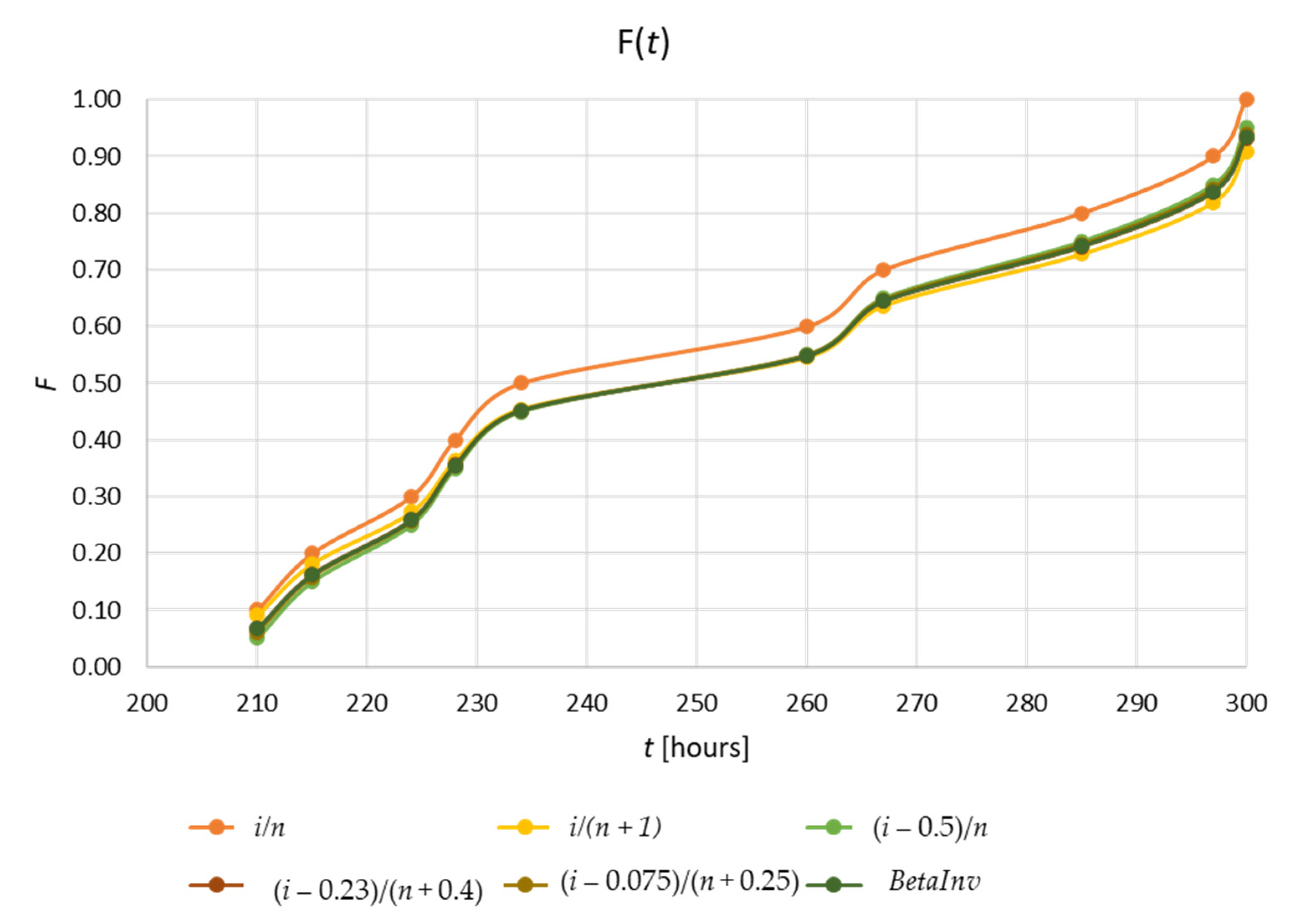
For a comparative analysis of the presented estimators, the values that re calculated in the case of a complete test of a batch of n = 10 products are presented, at which the failure times ti [hours] were recorded (Table 1) and the graphs for F(t) that were obtained with the respective estimators (Figure 2).

Table 1.
Distribution function estimator values F(t).
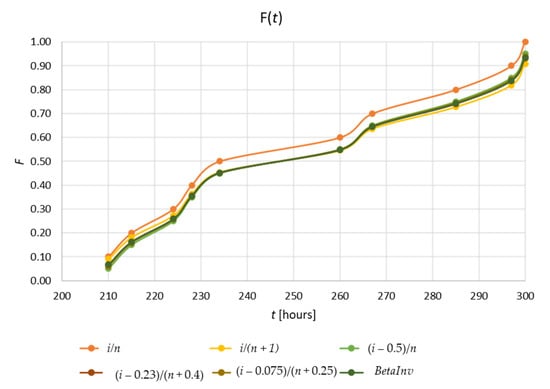
Figure 2.
Graphs of the distribution function F(t) that were obtained by various estimators.
Figure 2 shows that the “naive estimator” leads to clearly different results from all the other estimators, instead, all the other estimators are almost identical to the BETA.INV estimator. However, of these, the Benard estimator is most used to estimate the F(t) distribution function when the BETA.INV function is not available.
2.3. Determining the Parameters of the Three-Parametric Weibull Model
For this, the facility offered by the trendline function of Microsoft Excel will be used after the linearization of the Weibull distribution function by the method that is known and used almost invariably in Weibull modeling [24,25]: apply two successive logarithms of the reliability function given by the relation (1):
After the first logarithm results:
and, after the second logarithm, the final shape is obtained:
which represents a linear equation of form:
where:
It follows that in the probabilistic network having on the ordinate the Y scale and on the abscissa the X scale, a distribution of statistical data that are defined by the Weibull law of parameters γ, η, and β will be aligned after a line, also called “Weibull line”, having the inclination that is equal to the value of the parameter β.
The method to be proposed has as a starting point the observation that, under the conditions in which the parameter γ is initially determined, the analytical expression for the Weibull line is reduced to linear relation (13), which contains the shape parameter β and the scale parameter η. This means that the values of the parameters β and η can be determined by linear regression of point distribution Yi(Xi) using the “trendline” function that is available in current Microsoft Excel spreadsheets [26,27,28].
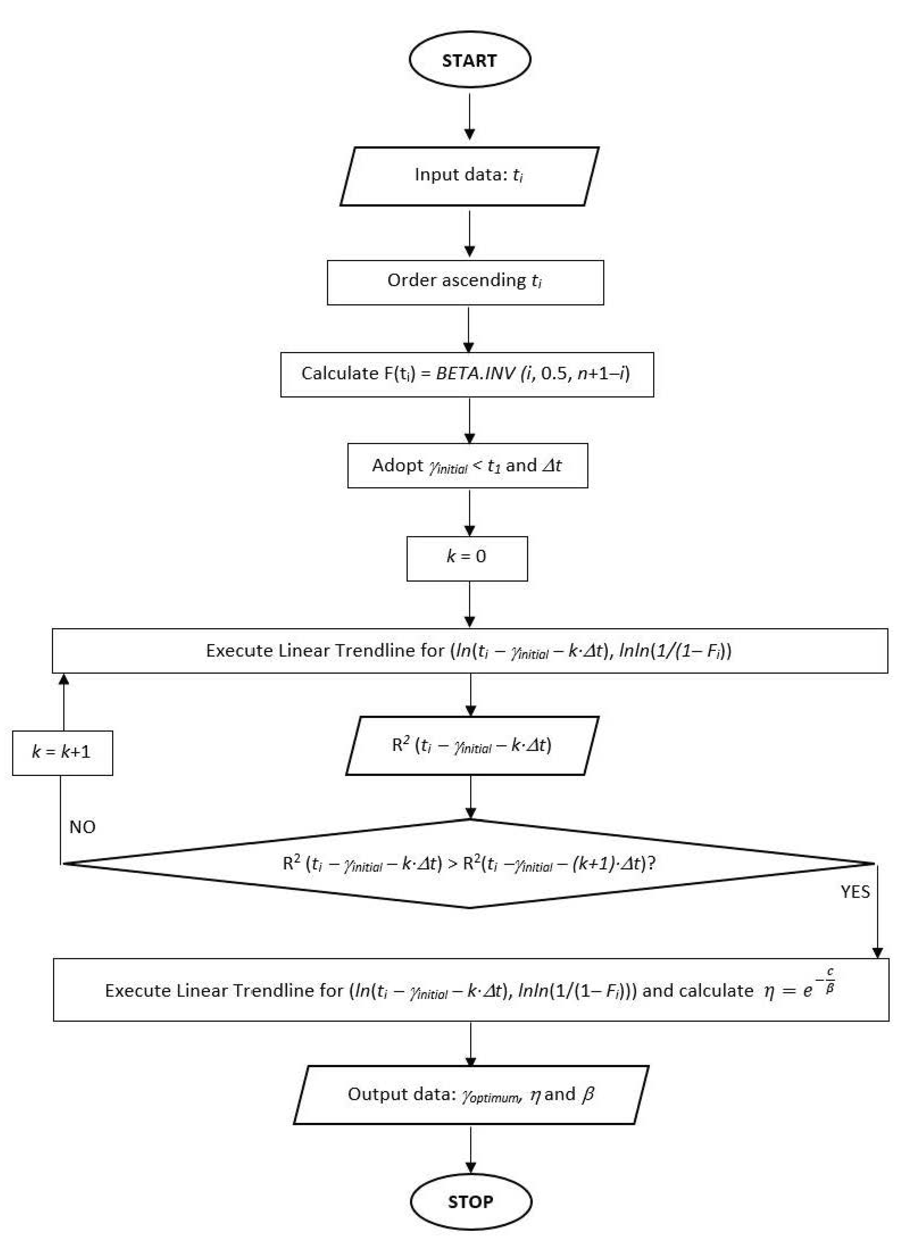
Figure 3 shows the flowchart for the proposed methodology, which could be easily translated into a calculation program.
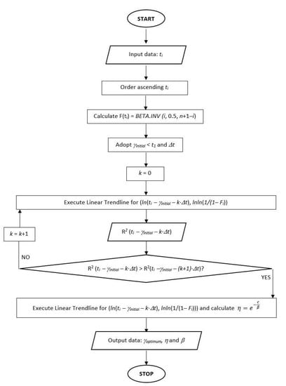
Figure 3.
Flowchart for the proposed methodology.
Thus, using the “trendline” function, the “linear” option is chosen, and the regression line of the point pair distribution (Xi, Yi) is constructed, for which the analytical relation and the value of the square of the degree of correlation are obtained R2.
According to relation (9), the coefficient of the variable X is the very parameter of the form β, and the free term contains the parameters β and η:
From this last relation, knowing the value of the parameter β the parameter η can be obtained analytically, according to the relation:
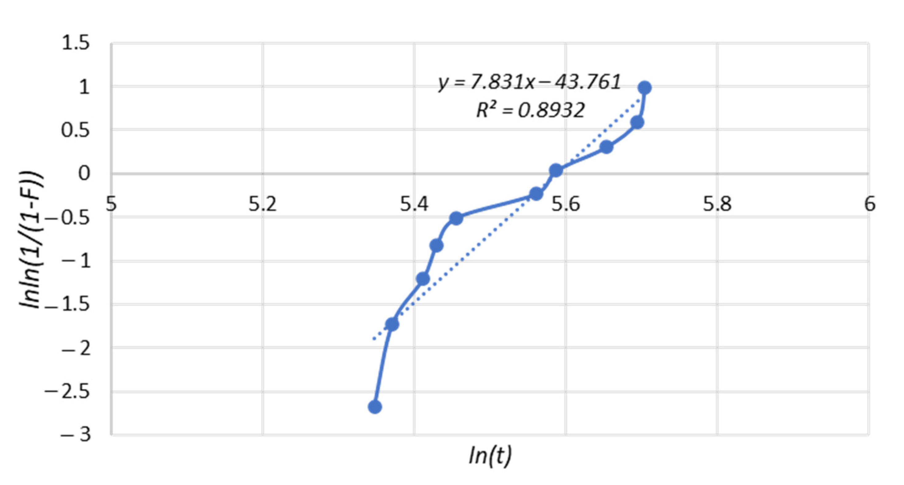
According to the proposed methodology, for the data ti (I = 1…10) that constitute the case study, the F(ti) estimator was determined using the BETA.INV function, and then, the quantities ln(ti) and ln [1/(1 − F)], presented in Table 2 with which the graph that is presented in Figure 3 was built.
Table 2.
Calculated values for estimating and linear regression of the distribution function F(t) for γ = 0.
Thus, for the data distribution that constitutes the case study, for the bi-parametric model (parameter γ = 0), the linear regression in the following figure shows the values of the two parameters: β = 7.831 and and a coefficient of determination R2 = 0.8932.
It is found that the parameter β has a value above 6—too high, as specified in the paper [2], so that the model does not have a proper probability (this is due to the fact that the first failure time is very long, relative to the amplitude distribution, which corresponds to a coefficient of variation ν= σ/m very small), which is confirmed both by the graphic image and by the low value of coefficient of determination: R2 = 0.8932. It is obvious that in this case, the bi-parametric Weibull model is inappropriate so it is necessary to adopt a three-parametric model, so a model in which to use the location parameter [9]. It will certainly provide a better likelihood degree. For the estimation of the third parameter (location), the existence of the parameter estimate is an important aspect. This is demonstrated in the paper [20]. There are various methods to identify this parameter, but are more laborious, including the one that is presented in the paper [11]. But very good results are also obtained by adopting for this parameter a value that is close to the first failure time, but strictly lower, because otherwise it will appear as the first value t − γ = 0, for which the logarithmic function is not defined.
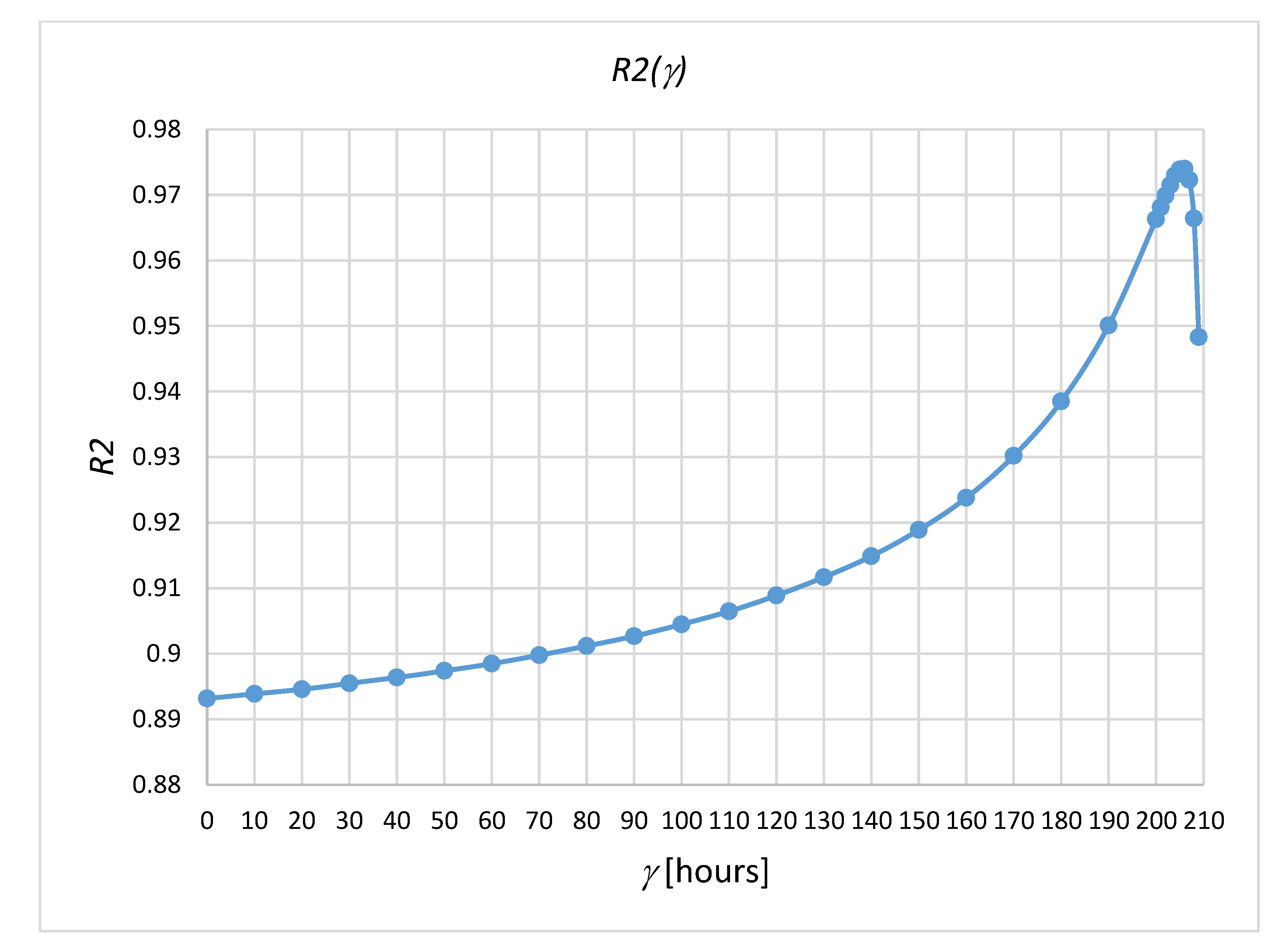
Thus, successively using the values for γ that are smaller than t1 = 210 h, the respective graphs were constructed in the same way as in Figure 4 and thus the respective values for the coefficient of determination were identified, identifying the highest value: for γ = 206 h, coefficient of determination is R2 = 0.9740, which is clearly superior to that which was obtained for the bi-parametric Weibull model (when γ = 0). Figure 5 shows the graph R2(γ) made for values γ tested starting with the one immediately below the first failure time, γ = 209 h, noting that the graph shows only one maximum, for γ = 206 h, after which, as the values γ decreases, follows a downward trend that touches for γ = 0 the value that is obtained for the case of the bi-parametric model (R2 = 0.8932).
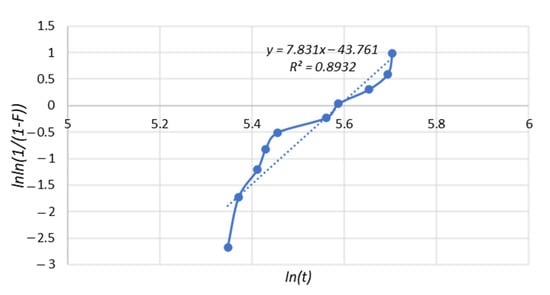
Figure 4.
Weibull bi-parametric and regression line graph.
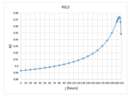
Figure 5.
Graph R2(γ), with the maximum value for R2 corresponding to the value γoptimum = 206 h.
According to the results that are presented in the literature by the correlation coefficient method, but were obtained by much more laborious calculations, including special calculation programs that were designed in Matlab [10], it is recommended to adopt for the location parameter a value that is close to the time of failure (strictly shorter than the first failure time), but the graph shows that this value does not have to be in the immediate vicinity of the moment t1. The optimum value can be obtained by successive tests (by probing), for values that are smaller and smaller in relation to the first failure time, until the values that are obtained for R2 begin to decrease, which confirms that the optimal value has been identified, which is unique.
Thus, after only five attempts with a step of 1 h, it is found, performing the linear regression for each step, that the optimal model was obtained on the fourth attempt (case γ = 206 h), for this optimal three-parametric model (those for which the coefficient of determination is maximum: R2 = 0.9740) resulting, after processing the data from the case study (Table 3) and performing the linear regression (Figure 6), in the values for the other two parameters:
Table 3.
Calculated values for estimating and linear regression of the distribution function F(t) for γoptimum = 206 h.
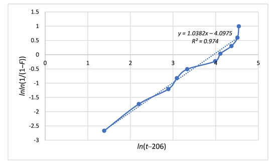
Figure 6.
Weibull three-parametric graph for γoptimum = 206 h and regression line.
- -
- shape parameter: β = 1.0382.
- -
- the scale parameter: .
Thus, it is found that, after determining the optimal value of the location parameter, by simply changing the variable, from t to (t − γ optimum), it is possible to operate in Microsoft Excel with the function corresponding to the bi-parametric Weibull model, and the operator is, in fact, even the optimal three-parametric model that is defined by the relation:
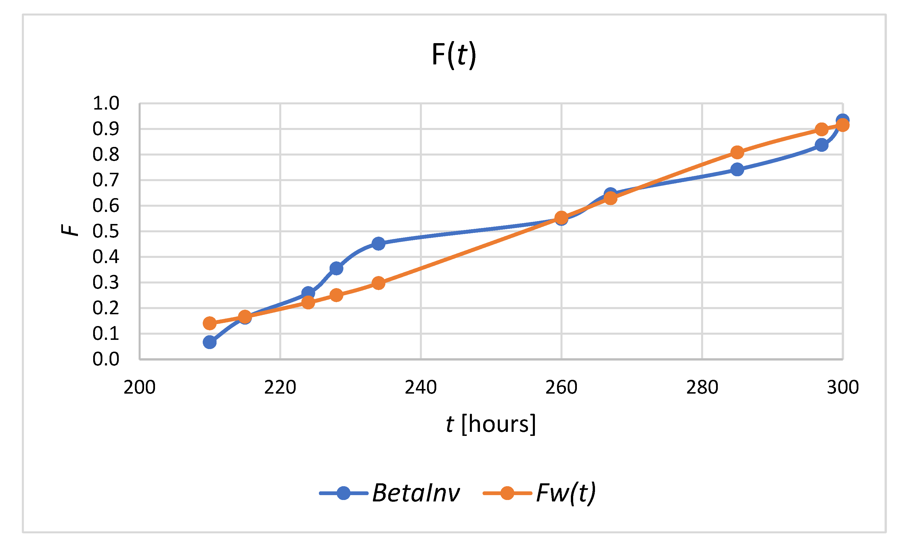
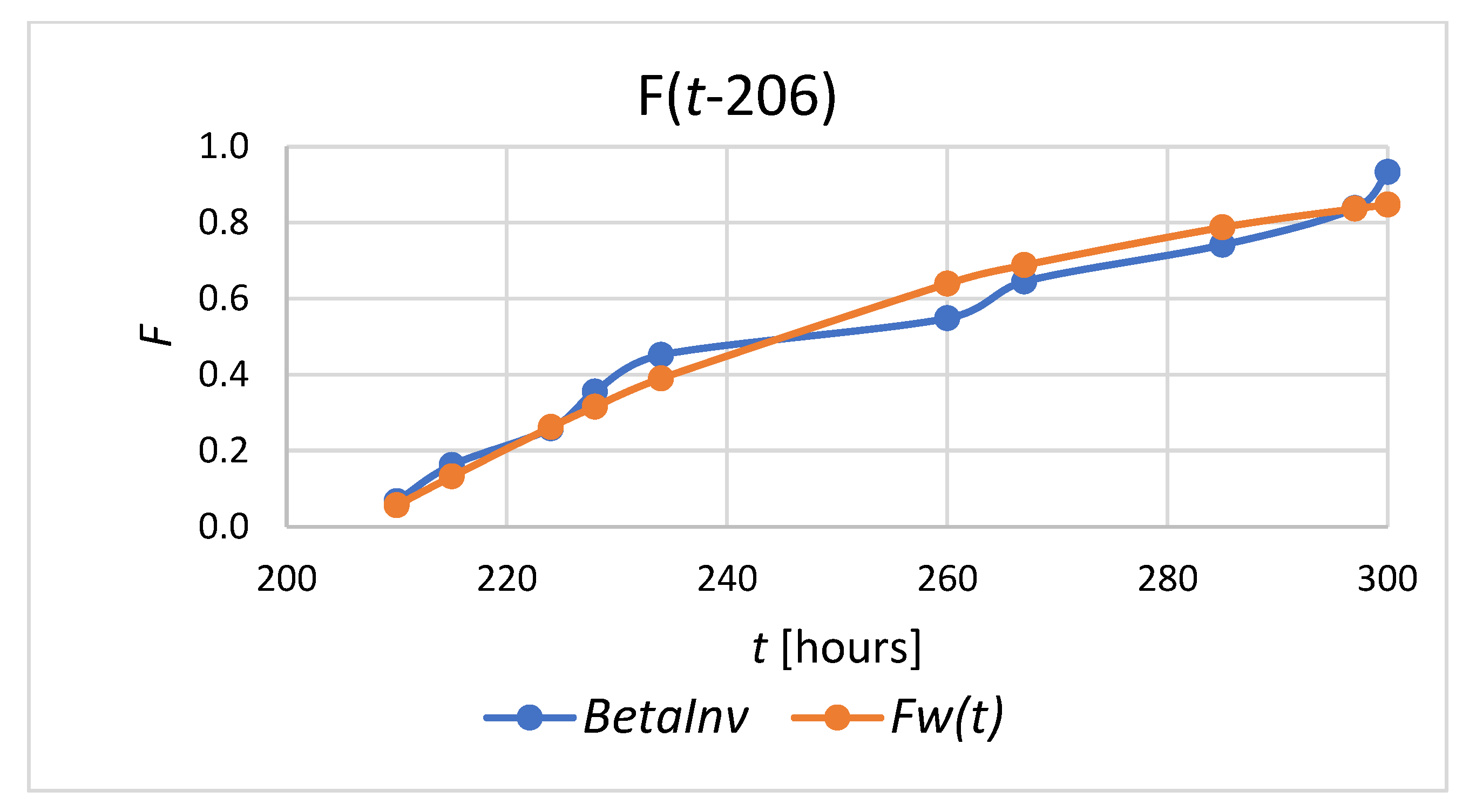
The fact that the Weibull three-parametric model with γ = 206 h is more suitable is also observed in the graphs below (Figure 7 and Figure 8), where the graphs for the distribution functions F(t) that were obtained on the two paths are presented: statistic (with BETA.INV function) and by bi-parametric Weibull modeling, for the argument t, respectively, for the argument (t-206), the last case being the Weibull three-parametric FW model for the parameter γ = 206.
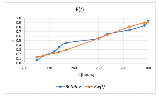
Figure 7.
Distribution function graphs F(t) that were obtained by the BETA.INV function and by the bi-parametric Weibull model (γ = 0).
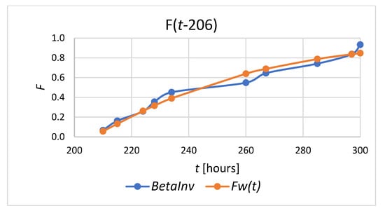
Figure 8.
Distribution function graphs F(t-206) that were obtained by the BETA.INV function and by the optimal three-parametric Weibull model (γoptimum = 206 h).
The data were obtained with the WEIBULL.DIST function (t; beta; eta; TRUE) from the Microsoft Excel calculation program (Table 4), according to the relation for the distribution function for the parametric Weibull model:
Table 4.
Values that were calculated for the distribution function F(t), for t, and (t – γoptimum).
With the help of the Excel CORREL function, the correlation coefficient was determined for the values that were obtained with the BETA.INV function and the two models that were obtained: for the bi-parametric Weibull model resulted in the value of 0.9719, while for the three-parametric Weibull model a value significantly higher, of 0.9838.
This supports the efficiency of the proposed method, for which the usual Microsoft Excel program is sufficient to arrive at a three-parameter Weibull model that is more likely than the two-parameter Weibull model.
3. Discussion
The theoretical and applied research that was conducted led to the following findings:
- In many works MR is approximated with various algebraic estimators (i.e., Benard, Hazen etc.), more or less adequate, but now the MR values can be accurately identified, using the BETA.INV function that is available in the Microsoft Excel calculator.
- The use of the location parameter is mandatory in some cases, such as for the product operability, where the location parameter shows the guaranteed operating time of the object.
- By representing in logarithmic coordinates, we determined three-parametric Weibull models for different values that were initially adopted for the location parameter.
- Using as a criterion the coefficient of determination that was obtained using the trendline function for the linear model, it was possible to identify, by successive tests, the optimal value of the location parameter.
- The accuracy with which the optimal parameter γoptimum is identified is equal to the value of the adopted step t by the user, which can be more or less fine, depending on the desired level of detail.
- The proposed methodology can be easily translated into a calculation program, as can be seen in the flowchart that was made.
4. Conclusions
The estimation of the failure time distribution function, F(t), can be done in the new versions of Microsoft Excel program by directly determining the Median Ranks estimator through the BETA.INV function for the case of the median probability, equal to 0.5.
As a result, using the exact values for Median Ranks, and not estimated by various algebraic estimators (Benard, Hazen, etc.), a more appropriate reliability model will be obtained.
By the well-known graphic-analytical method for estimating the two-parametric Weibull model, the two parameters can be identified—the shape parameter and the scale parameter—but it is possible to identify an appropriate three-parametric model (which also contains the location parameter) by the method that is presented. The optimum value of the location parameter corresponds to the three-parametric Weibull model resulting from the linear regression of the distribution function for which the coefficient of determination value is maximum.
To identify the optimal location parameter, an iteration method was proposed, with a predetermined step and starting with a value that was immediately lower than the first failure time, the results confirming that after a small number of attempts the value of the location parameter is leading to the most likely three-parametric Weibull model.
The applicability of the method can be further improved by transposing it into a calculation program, according to the presented logic scheme.
In this way, a precise and easily applicable method has been created by which an appropriate three-parametric Weibull model can be identified using the current features of Microsoft Excel.
Author Contributions
Conceptualization, A.B. and S.T.; methodology, A.M.T. and A.B.; software, A.B. and S.T.; validation, A.M.T. and M.D.; formal analysis, A.A.B.; investigation, A.B.P.; resources, A.M.T. and A.B.; data curation, A.B.P. and S.T.; writing-original draft preparation, A.B.; writing-review and editing, A.M.T. and A.B.P.; visualization, A.M.T. and M.D.; supervision, A.M.T.; project administration, A.M.T., A.B.P., and S.T. All authors have read and agreed to the published version of the manuscript.
Funding
This research received no external funding.
Institutional Review Board Statement
Not applicable.
Informed Consent Statement
Not applicable.
Data Availability Statement
Not applicable.
Conflicts of Interest
The authors declare no conflict of interest.
References
- Basumatary, H.; Sreevalsan, E.; Sasi, K.K. Weibull parameter estimation—A comparison of different methods. Wind Eng. 2005, 29, 309–315. [Google Scholar] [CrossRef]
- IEC 61649:2008; Weibull Analysis. IEC: Geneva, Switzerland, 2008.
- Elmahdy, E.E. A new approach for Weibull modeling for reliability life data analysis. Appl. Math. Comput. 2015, 250, 708–720. [Google Scholar] [CrossRef]
- Elsayed, A.E. Reliability Engineering; John Wiley & Sons: Hoboken, NJ, USA, 2012. [Google Scholar]
- Evans, J.W.; Kretschmann, D.E.; Green, D.W. Procedures for Estimation of Weibull Parameters; USDA Forest Service, Forest Products Laboratory: Madison, WI, USA, 2019. [Google Scholar] [CrossRef]
- Fernandez, A.; Vazquez, M. Improved Estimation of Weibull Parameters Considering Unreliability Uncertainties. IEEE Trans. Reliab. 2011, 61, 32–40. [Google Scholar] [CrossRef]
- Lei, Y. Evaluation of three methods for estimating the Weibull distribution parameters of Chinese pine (Pinus tabulaeformis). J. For. Sci. 2008, 54, 566–571. [Google Scholar] [CrossRef]
- McCool, J.I. Inference on the Weibull Location Parameter. J. Qual. Technol. 1998, 30, 119–126. [Google Scholar] [CrossRef]
- Morariu, C.O.; Şimon, A.E. Estimation of the Weibull Location Parameter through the Correlation Coefficient Method. Bull. Transilv. Univ. Brașov 2004, 11, 187–190. [Google Scholar]
- Palisson, F. Détermination des paramètres du modèle de Weibull à partir de la méthode de l’actuariat, Revue de statistique appliquée. Tome 1989, 37, 5–39. Available online: http://www.numdam.org/article/RSA_1989__37_4_5_0.pdf (accessed on 20 January 2022).
- Pobočíková, I.; Sedliačková, Z. Comparison of four methods for estimating the Weibull distribution parameters. Appl. Math. Sci. 2014, 8, 4137–4149. [Google Scholar] [CrossRef]
- Westfall, P.; Henning, K. Understanding Advanced Statistical Methods; CRC Press: Boca Raton, FL, USA, 2013; ISBN 9781466512108. [Google Scholar]
- Liu, S.; Wu, H.; Meeker, W.Q. Understanding and Addressing the Unbounded “Likelihood” Problem. Am. Stat. 2015, 69, 191–200. [Google Scholar] [CrossRef]
- Zaiontz, C. Fitting a Weibull Distribution via Regression. 2021. Available online: https://www.real-statistics.com/distribution-fitting/fitting-weibull-regression/ (accessed on 20 January 2022).
- Zhao, J. Robust Parameter Estimation in the Weibull and the Birnbaum-Saunders Distribution. Master’s Thesis, Clemson University, Clemson, SC, USA, 2012. [Google Scholar]
- Assis, R.; Marques, P.C. A Dynamic Methodology for Setting Up Inspection Time Intervals in Conditional Preventive Maintenance. Appl. Sci. 2021, 11, 8715. [Google Scholar] [CrossRef]
- Rantini, D.; Iriawan, N. Irhamah On the Reversible Jump Markov Chain Monte Carlo (RJMCMC) Algorithm for Extreme Value Mixture Distribution as a Location-Scale Transformation of the Weibull Distribution. Appl. Sci. 2021, 11, 7343. [Google Scholar] [CrossRef]
- Villa-Covarrubias, B.; Piña-Monarrez, M.R.; Barraza-Contreras, J.M.; Baro-Tijerina, M. Stress-Based Weibull Method to Select a Ball Bearing and Determine Its Actual Reliability. Appl. Sci. 2020, 10, 8100. [Google Scholar] [CrossRef]
- Sourri, P.; Argyri, A.A.; Panagou, E.Z.; Nychas, G.-J.E.; Tassou, C.C. Alicyclobacillus acidoterrestris Strain Variability in the Inactivation Kinetics of Spores in Orange Juice by Temperature-Assisted High Hydrostatic Pressure. Appl. Sci. 2020, 10, 7542. [Google Scholar] [CrossRef]
- Park, C. A Note on the Existence of the Location Parameter Estimate of the Three-Parameter Weibull Model Using the Weibull Plot. Math. Probl. Eng. 2018, 2018, 6056975. [Google Scholar] [CrossRef]
- Barraza-Contreras, J.M.; Piña-Monarrez, M.R.; Molina, A. Fatigue-Life Prediction of Mechanical Element by Using the Weibull Distribution. Appl. Sci. 2020, 10, 6384. [Google Scholar] [CrossRef]
- Molina, A.; Piña-Monarrez, M.R.; Barraza-Contreras, J.M. Weibull S-N Fatigue Strength Curve Analysis for A572 Gr. 50 Steel, Based on the True Stress—True Strain Approach. Appl. Sci. 2020, 10, 5725. [Google Scholar] [CrossRef]
- Zhao, Q.; Jia, X.; Cheng, Z.; Guo, B. Bayesian Estimation of Residual Life for Weibull-Distributed Components of On-Orbit Satellites Based on Multi-Source Information Fusion. Appl. Sci. 2019, 9, 3017. [Google Scholar] [CrossRef]
- Ono, K. A Simple Estimation Method of Weibull Modulus and Verification with Strength Data. Appl. Sci. 2019, 9, 1575. [Google Scholar] [CrossRef]
- Bokde, N.; Feijóo, A.; Villanueva, D. Wind Turbine Power Curves Based on the Weibull Cumulative Distribution Function. Appl. Sci. 2018, 8, 1757. [Google Scholar] [CrossRef]
- Song, K.Y.; Chang, I.H.; Pham, H. A Software Reliability Model with a Weibull Fault Detection Rate Function Subject to Operating Environments. Appl. Sci. 2017, 7, 983. [Google Scholar] [CrossRef]
- Dubey, S.D. Hyper-efficient estimator of the location parameter of the weibull laws. Nav. Res. Logist. Q. 1966, 13, 253–264. [Google Scholar] [CrossRef]
- Dubey, S.D. On some statistical inferences for weibull laws. Nav. Res. Logist. Q. 1966, 13, 227–251. [Google Scholar] [CrossRef]


Publisher’s Note: MDPI stays neutral with regard to jurisdictional claims in published maps and institutional affiliations. |
© 2022 by the authors. Licensee MDPI, Basel, Switzerland. This article is an open access article distributed under the terms and conditions of the Creative Commons Attribution (CC BY) license (https://creativecommons.org/licenses/by/4.0/).