Article

A Novel Multi-Sensor Data-Driven Approach to Source Term Estimation of Hazardous Gas Leakages in the Chemical Industry

1
Department of Automatic Control and Systems Engineering, University of Sheffield, Sheffield, S1 3JD, UK
2
School of Information Science and Engineering, East China University of Science and Technology, Shanghai 200237, China
*
Author to whom correspondence should be addressed.
Processes 2022, 10(8), 1633; https://doi.org/10.3390/pr10081633
Submission received: 27 July 2022 / Revised: 6 August 2022 / Accepted: 9 August 2022 / Published: 17 August 2022

Abstract

:
Source term estimation (STE) is crucial for understanding and addressing hazardous gas leakages in the chemical industry. Most existing methods basically use an atmospheric transport and dispersion (ATD) model to predict the concentrations of hazardous gas leakages from different possible sources, compare the predicted results with multi-sensor data, and use the deviations to search and derive information on the real sources of leakages. Although performing well in principle, complicated computations and the associated computer time often make these methods difficult to apply in real time. Recently, many machine learning methods have also been proposed for the purpose of STE. The idea is to build offline a machine-learning-based STE model using data generated with a high-fidelity ATD model and then apply the machine learning model to multi-sensor data to perform STE in real time. The key to the success of a machine-learning-based STE is that the machine-learning-based STE model has to cover all possible scenarios of concern, which is often difficult in practice because of unpredictable environmental conditions and the inherent robust problems with many supervised machine learning methods. In order to address challenges with the existing STE methods, in the present study, a novel multi-sensor data-driven approach to STE of hazardous gas leakages is proposed. The basic idea is to establish a multi-sensor data-driven STE model from historical multi-sensor observations that cover the situations known as the independent hazardous-gas-leakage scenarios (IHGLSs) in a chemical industry park of concern. Then the established STE model is applied to online process multi-sensor data and perform STE for the chemical industry park in real time. The new approach is based on a rigorous analysis of the relationship between multi-sensor data and sources of hazardous gas leakages and derived using advanced data science, including unsupervised multi-sensor data clustering and analysis. As an example of demonstration, the proposed approach is applied to perform STE for hazardous gas-leakage scenarios wherein a Gaussian plume model can be used to describe the atmospheric transport and dispersion. Because of no need of ATD-model-based online optimization and supervised machine learning, the new approach can potentially overcome many problems with existing methods and enable STE to be literally applied in engineering practice.

1. Introduction

In the chemical industry, hazardous gas leakages are one of major causes of environmental pollution and serious accidents [1,2,3]. In order to address this problem, multi-sensors are often used to measure the concentrations of hazardous gas at different locations in the chemical industry parks to support risk assessment, hazard warning, and, more importantly, source term estimation (STE). The goal of STE is to estimate the parameters that describe the sources of leakages: namely, the location and strength of leakages. The results are crucial for identifying the cause of leakages so as to fundamentally resolve the hazardous gas leakages that have to be dealt with in a timely fashion [4,5].
Currently, most methods of STE mainly use a network of hazardous gas concentration sensors. The multi-sensor data are fused with prior information, such as meteorological data, to estimate the parameters of the sources of leakages using either an optimization approach or a Bayesian-inference-based probabilistic method [6,7,8]. The application of these methods to perform STE needs to use an atmospheric transport and dispersion (ATD) model or an inverse source-receptor model to generate the predicted concentrations of gas leakages from different possible sources. The predicted concentrations are then compared with the multi-sensor observations, and the deviations are used to search and derive the parameters of the sources of leakages that minimize a cost or likelihood function [9]. Based on this approach, many methods have been developed. For example, in [10], a hybrid genetic algorithm with composite cost functions was applied to improve the search for optimal solutions to the parameters of the sources of leakages. In [11], the optimization performance of the particle swarm optimization (PSO), the Nelder–Mead (NM) simplex method, and the PSO–NM hybrid algorithm were evaluated when applied to STE for the case where the Gaussian puff dispersion model can be used as the ATD model. In [12], an inverse-source-term-estimation method was applied to the data from wind tunnel experiments for STE. The inverse method uses the concept of the “source-receptor functions” (SRFs), which describe the sensitivity of concentration at a receptor to the parameters of the emitting source. This can resolve the difficulties with using a forward ATD model when the number of the locations of potential hazardous-gas-leakage sources is considerable. Recently, many machine-learning-based STE methods have also been developed. These methods include, for example, deep-neural-network- and random-forest-classifier-based STE in chemical industrial parks [13], federated-learning-based STE in urban environments [14], convolutional-neural-network-based STE with obstacles [15], back-propagation neural-network-based-STE for nuclear accidents [16], and recurrent neural-network-based-STE for severe nuclear accidents [17]. The basic idea of machine-learning-based STE is to offline train a machine learning STE model and apply the machine learning model online to process multi-sensor data and carry out STE. The machine learning STE model is often trained using the data generated by a high-fidelity ATD model, such as a computational fluid dynamic (CFD) model, and, in principle, the data have to cover all leakage scenarios of concern.
In principle, the ATD-model-based-STE methods require running an ATD or an inverse model online in conjunction with an optimization or Bayesian inference framework [7,18]. The complexity associated with the ATD model itself, as well as carrying out a sophisticated optimization or Bayesian inference, implies that there is a significant issue with the practical application of these existing STE methods. Consequently, although most of these STE methods perform well in theory, because of the complicated computations needed and the associated computer time required, these methods are often difficult to apply in practice to analyze multi-sensor data and carry out STE in real time [19]. Machine-learning-based STE can work well, provided that the data that have been used to train the machine learning STE model are fully representative of all leakage scenarios in the chemical industry park of concern. This is, however, often difficult in practice because of the complexity of hazardous gas leakages and uncertainties in sensor data due to noises and unpredictable environmental conditions. This and the well-known issue of poor robustness with machine learning models in many practical applications [20] imply that the application of machine-learning-based STE in engineering practice is also a difficult task.
Motivated by the need to address these challenges with existing STE studies, in the present study, a novel multi-sensor data-driven approach to the STE of hazardous gas leakages in the chemical industry is proposed. The idea is to:
  • offline establish a multi-sensor data-driven STE model from historical multi-sensor data measured during a period that covers the situations known as independent hazardous-gas-leakage scenarios (IHGLSs) in a chemical industry park and then
  • online apply the established STE model to process field-measured multi-sensor data and determine the leak sources and associated parameters in real-time.
The IHGLSs are a new concept introduced in the present study, which refers to the hazardous-gas-leakage scenarios in a chemical industry park that are linearly independent. The building of the offline multi-sensor data-based STE model basically requires the completion of three tasks. First, advanced multi-sensor data analysis is applied to (1) find the number of IHGLSs over the period when the historical multi-sensor data are collected from the chemical industry park and (2) determine the most-representative multi-sensor data measurements for each of these IHGLSs. Secondly, a STE approach is applied offline to determine the parameters of the sources of leakages associated with each of these IHGLSs from the corresponding multi-sensor data measurements. Finally, the results obtained in the first two steps are used to produce a multi-sensor data-driven STE model that can be applied in real time to perform STE from multi-sensor data measured in the chemical industry park at any time. Because the STE in the second task is conducted offline, any existing approach can be applied as needed without any concern regarding time constraints. The well-known difficulties with the ATD-model-based-STE methods can therefore be resolved. In addition, because the multi-sensor data-driven STE modeling involves no supervised learning, the issues of possible poor robustness with machine-learning-based STEs can also be circumvented. Consequently, the new approach can potentially overcome many problems with the existing methods and enable STE to be literally applied in engineering practice.
In this paper, the basic idea and the novelty of the new multi-sensor data-driven approach is first introduced and illustrated using a simple example in Section 2. Then, in Section 3, the STE problem that will be addressed is defined. Significant relationships between the multi-sensor data and the sources of hazardous gas leakages in a chemical industry park are derived, providing an important basis for the development of the new multi-sensor data-driven approach to STE. After that, in Section 4, the new approach and the associated implementation algorithm are proposed. In Section 5, numerical simulation studies are conducted wherein the proposed approach is applied to perform STE for hazardous gas-leak scenarios when there exist two leaking sources and when gas dispersion follows a Gaussian plume model. The results verify the effectiveness of the proposed approach and demonstrate its potential significance in practical applications. Moreover, the nature and advantages of the proposed approach are discussed in Section 6. Finally, conclusions are summarized in Section 7.

2. Basic Idea and Novelty

We can imagine a chemical industrial park where there are S possible hazardous-gas-leaking sources. N sensors are fitted in the chemical industrial park to monitor hazardous gas concentrations at N different locations. Here, the STE problem is concerned with the determination of the location and strength of hazardous gas leakages from S ¯ S leaking sources using the measured data from the N sensors.
In order to better introduce the basic idea and novelty of the proposed multi-sensor data-driven STE, first it is necessary to look at one of typical solutions to the STE problem, which basically involves the following steps [10,11,12]:
(1)
Building an ATD model that describes the transport and dispersion of hazard gas in the chemical industrial park;
(2)
Using the ATD model to generate the concentration data of hazardous gas that would be measured at the N different sensor locations, when hazardous gas leakages take place from different possible sources under a given meteorological condition;
(3)
Applying an optimization approach to search for the strengths of hazardous gas leakages Q i *   i { 1 , 2 , , S } in the S possible leaking sources, such that the differences between the concentrations of hazardous gas generated by the ATD model and the practically measured multi-sensor data at the N different sensor locations reach a minimum.
The solution is illustrated in Figure 1 which, in principle, works well but has a significant issue in practical applications. This is due to the amount of time needed to run the ATD model to generate the concentration data of hazardous gas in Step (2) and to implement the optimization approach in Step (3). For performing STE once from one set of practically measured multi-sensor data, running a complicated ATD model and associated optimization routine may take time, from hours to days, making the STE solution difficult to be applied and implemented in real time [8,10].
The present study of a multi-sensor data-driven STE follows the same physical principle as applied by these typical solutions but aims to resolve the afore-mentioned significant challenges with these existing STE approaches. The novel idea is to:
(a)
build a multi-sensor data-driven STE model from (1) historical multi-sensor data measured during a period that covers the IHGLSs of concern and (2) the STE outcomes determined offline using an ATD-model-based STE method from the multi-sensor data collected in these IHGLSs
(b)
apply the STE model to online-measured multi-sensor data in the chemical industry park to perform STE in real time.
Because the ATD-model-based STE is carried out offline, computation issues with running a complicated ATD model and an associated optimization routine are not a problem anymore. The new approach can potentially overcome the bottleneck problems with existing ATD-model-based STE approaches.
In order to explain this novel idea in a bit more detail, we can consider the case where S = 2, i.e., there are two possible hazardous gas-leakage sources A and B in a chemical industry park. The coordinate and hazardous gas-leakage strength of source A are ( x A , y A , z A ) and Q A , respectively, while the coordinate and hazardous gas-leakage strength of source B are ( x B , y B , z B ) and Q B , respectively. In this case:
  • there exist only two hazardous-gas-leakage scenarios that are linearly independent, so there are two IHGLSs;
  • the multi-sensor data collected in the two IHGLSs can be used to represent multi-sensor data collected in any other leakage scenario.
These two points are an important basis for the new idea of a multi-sensor data-driven STE introduced in the present study.
To demonstrate the validity of the two points, we can consider the hazardous gas-leakage situations wherein a Gaussian plume model can be used as the ATD model to represent the transport and dispersion of leaking hazardous gases. In these situations, the concentrations of a leaking hazardous gas measured by sensor i, i = 1, …, N, can be described as:
C ( i ) = Q A 2 π v σ y A i σ z A i e ( y i y A ) 2 2 σ y A i 2 [ e ( z i z A ) 2 2 σ z A i 2 + e ( z i + z A ) 2 2 σ z A i 2 ] + Q B 2 π v σ y B i σ z B i e ( y i y B ) 2 2 σ y B i 2 [ e ( z i z B ) 2 2 σ z B i 2 + e ( z i + z B ) 2 2 σ z B i 2 ] i = 1 , , N
where C ( i ) is the concentration of the leaking hazardous gas measured by the ith sensor located at ( x i , y i , z i ) , v is wind speed, and σ y A i = a ( x i x A ) b , σ z A i = c ( x i x A ) d , σ y B i = a ( x i x B ) b , σ z B i = c ( x i x B ) d . where a , b , c , d are the dispersion coefficients, which are a function of the atmospheric environment that can be determined by either experiences or experiments.
Two IHGLSs in this situation can be, e.g., Scenario I, where Q A = Q ¯ A 0 and Q B = 0 , and Scenario II where Q A = 0 and Q B = Q _ ¯ B 0 . This is because vectors [ Q ¯ A , 0 ] and [ 0 , Q _ ¯ B ] are linearly independent. We represent the multi-sensor data collected in the two IHGLSs as C ¯ 1 ( i ) ,   i = 1 , , N and C ¯ 2 ( i ) ,   i = 1 , , N , respectively. It is known from ATD model (1) that:
C ¯ 1 ( i ) = Q ¯ A 2 π v σ y A i σ z A i e ( y i y A ) 2 2 σ y A i 2 [ e ( z i z A ) 2 2 σ z A i 2 + e ( z i + z A ) 2 2 σ z A i 2 ] , i = 1 , , N
C ¯ 2 ( i ) = Q ¯ B 2 π v σ y B i σ z B i e ( y i y B ) 2 2 σ y B i 2 [ e ( z i z B ) 2 2 σ z B i 2 + e ( z i + z B ) 2 2 σ z B i 2 ] , i = 1 , , N
Moreover, it is known from Equations (1)–(3) that:
C ( i ) = α C ¯ 1 ( i ) + β C ¯ 2 ( i ) , i = 1 , , N ,  
where α = Q A Q ¯ A , β = Q B Q ¯ B . Therefore, as stated by the second of the two points above, the multi-sensor data C ( i ) ,   i = 1 , , N measured at any leaking scenario can be represented by C ¯ 1 ( i ) ,   i = 1 , , N and C ¯ 2 ( i ) ,   i = 1 , , N , which are the multi-sensor data collected in two IHGLSs.
The two points’ statement above implies that if one can find multi-sensor measurements from IHGLSs and know the STE results corresponding to each of these IHGLSs, then the relationship (4) can be exploited to realize STE for any hazardous gas-leakage scenarios of concern when given the multi-senor data collected from these hazardous gas-leakage scenarios. To explain this, rewriting Equation (4) in a matrix form as:
[ C ( 1 ) C ( N ) ] = [ C ¯ 1 ( 1 ) C ¯ 2 ( 1 ) C ¯ 1 ( N ) C ¯ 2 ( N ) ] [ α β ]
and solving Equation (5) for α ,   β yields
[ α β ] = [ Q A / Q ¯ A Q B / Q ¯ B ] = ( C ¯ C ¯ T ) 1 C ¯ [ C ( 1 ) C ( N ) ]
where C ¯ = [ C ¯ 1 ( 1 ) C ¯ 1 ( N ) C ¯ 2 ( 1 ) C ¯ 2 ( N ) ] .
From Equation (6), it can be readily shown that
[ Q A Q B ] ( i ) = [ Q ¯ A 0 ( i i ) 0 Q ¯ B ( i i i ) ] ( C ¯ C ¯ T ) 1 C ¯ ( i v ) [ C ( 1 ) C ( N ) ] ( v )
As mentioned above regarding the implication of the two points’ statement, Equation (7) clearly indicates that the STE outcome (i) from any multi-sensor observations (v) can be determined from this equation using the STE outcomes for two IHGLSs (ii) and (iii) and the multi-sensor data collected in the two IHGLSs (iv).
Basically Equation (7) is a specific form of the multi-sensor data-driven STE model mentioned in point (a) of the multi-sensor data-driven STE idea. In this specific case, the model is composed of the multi-sensor sensor data contained in matrix C ¯ , which are collected from two IHGLSs and the STE outcomes [ Q ¯ A , 0 ] T and [ 0 , Q ¯ B ] T for the two IHGLSs. The model input is any set of multi-sensor observations [ C ( 1 ) , , C ( N ) ] T , and the model output is the STE outcome [ Q A , Q B ] T from this set of multi-sensor observations. Therefore, the model can be directly applied to online-measured multi-sensor data to perform STE in real time, which is point (b) of the multi-sensor data-driven STE idea.
Clearly, building a multi-sensor data-driven STE model like (7) is the key to the implementation of multi-sensor data-driven STE. To achieve this objective, generally speaking, the following tasks are required:
(i)
determining the number of IHGLSs from the historical multi-sensor data measured during a period of time that covers the IHGLSs of concern;
(ii)
finding the multi-sensor data collected from each of these IHGLSs;
(iii)
determining the STE result for each of the IHGLSs; and finally
(iv)
building the STE model using the results of (i)–(iii) and applying the model online to perform STE in real time.
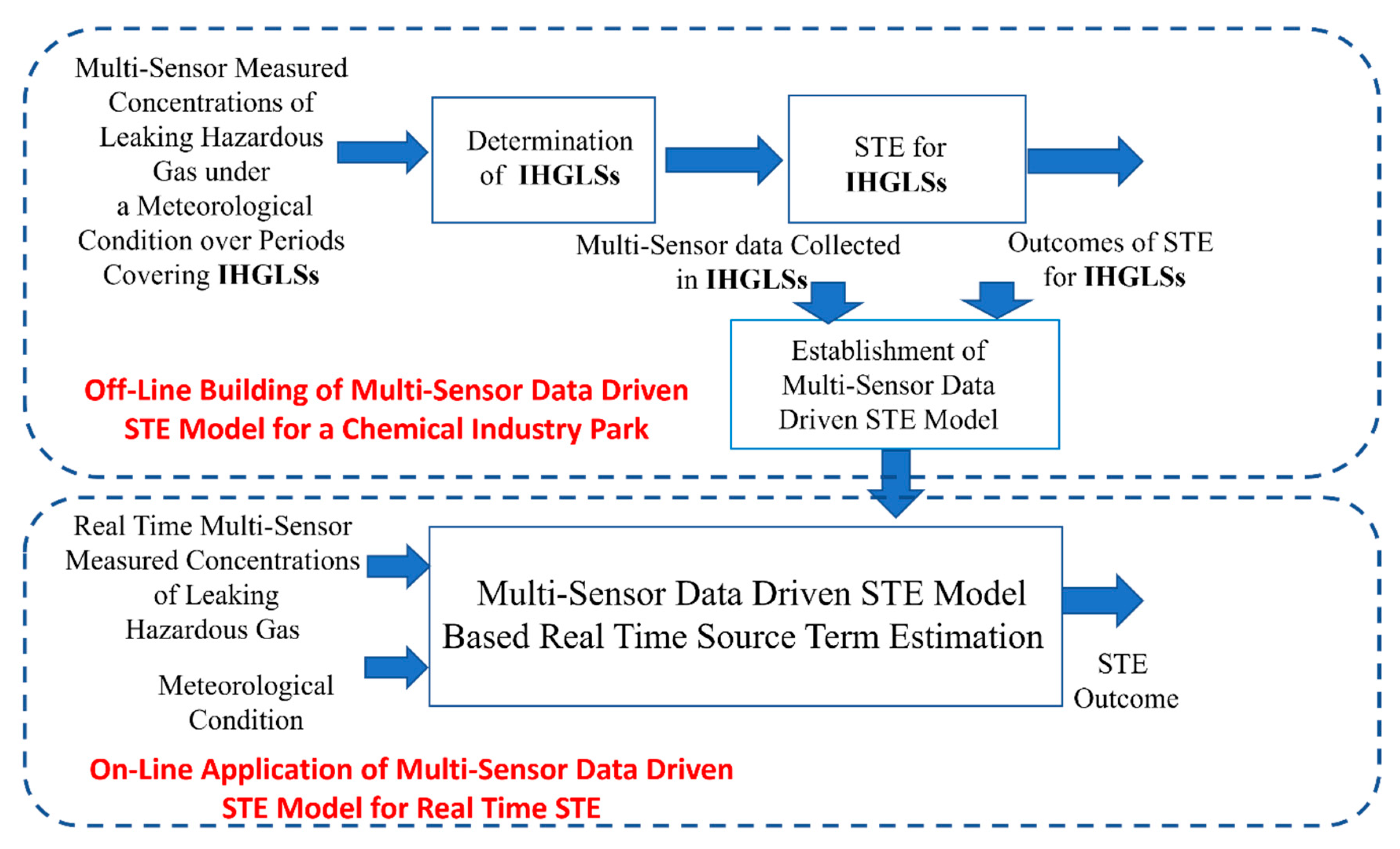
Figure 2 illustrates the novel idea of the proposed multi-sensor data-driven STE involving offline multi-sensor data-driven STE-model building, as well as the online application of the offline-built multi-sensor data-driven STE model to perform STE in real time. The multi-sensor data-driven model is determined offline using the outcomes of tasks (i) and (ii), that is, multi-sensor data collected during IHGLSs, as well as the result of task (iii), that is, STE outcomes for the IHGLSs. Because of the lack of a time constraint with offline operations, one can apply any STE method to produce the STE outcomes needed for building the multi-sensor data-driven STE model. In addition, because the online application of the multi-sensor data-driven STE model has no need for an ATD model and online optimization as in the case of the conventional STE shown in Figure 1, the proposed multi-sensor data-driven STE can readily achieve STE in real time. This is expected to resolve the difficulties with many existing STE techniques.
It is worth noting that IHGLSs are meteorological-condition-dependent. Under different meteorological conditions, the multi-sensor data-driven STE model built in the offline model-building stage is different. Therefore, in the real-time application of the multi-sensor data-driven model for STE, the meteorological condition is needed to identify the multi-sensor data-driven STE model corresponding to this meteorological condition. It is the multi-sensor data-driven STE model corresponding to this meteorological condition that is needed to produce the STE outcome.
In the next section, on the basis of the conceptual introduction above, the multi-sensor data-driven STE problem will be formally defined to facilitate the development of the novel multi-sensor data-driven STE approach in the later parts of this paper.

3. Problem Definition and Relationships between Multi-Sensor Data and Hazardous Gas Leakages

We can consider the scenarios in a chemical industry park where hazardous gas leakages take place from S possible leaking sources, and the following assumptions are valid.
(1)
The meteorological condition in terms of wind speed and wind direction is known.
(2)
Under this meteorological condition, the hazardous gas leakages from the S possible leaking sources can be detected by N ¯ sensors with N N ¯ S   .
(3)
M > N sets of historical multi-sensor data have been collected over a period from the chemical industry park under this meteorological condition.
(4)
Over the period when the M sets of historical multi-sensor data were collected, there exist hazardous gas leakages from S ¯ leaking sources with S ¯ S   .
(5)
Among the M sets of collected multi-sensor data, there are S ¯ sets of data that can cover S ¯ IHGLSs. This implies that vectors [ Q ¯ 1 ( j ¯ ) , , Q ¯ S ¯ ( j ¯ ) ] , j ¯ = 1 , , S ¯ are linearly independent, where Q ¯ i ¯ ( j ¯ ) ( i ¯ = 1 , , S ¯ , j ¯ = 1 , , S ¯ ) represents the strength of the hazardous gas leakage from the i ¯ th of the S ¯ leaking sources in the j ¯ th of the S ¯ hazardous-gas-leakage scenarios.
(6)
The concentration of hazardous gas at any location in the chemical industry park produced by hazardous gas leakages from all of the S possible leaking sources equals to the summation of S individual concentrations of hazardous gas at this location. Each of the S individual concentrations is the concentration of hazardous gas at the same location produced by hazardous gas leakage from each of the S possible sources.
Under these assumptions, the STE problem to solve here is concerned with how to establish a multi-sensor data-driven STE model from the M sets of historical multi-sensor data and apply the model to practically measured multi-sensor data to perform STE in real time.
Three key issues with the STE model building and application are determining S ¯ , finding the multi-sensor data collected from S ¯ IHGLSs, and associating real-time measured multi-sensor data with the outcome of STE using the STE model. These issues can be addressed based on the relationships between multi-sensor data and the sources of hazardous gas leakages described in Proposition 1 as follows.
Proposition 1:
Under Assumptions (1)–(6), denote the M sets of multi-sensor data specified in Assumption (3) as C j ( 1 ) , , C j ( N ) j = 1 , , M
, define matrix:
C = [ C 1 ( 1 ) C 1 ( N ) C M ( 1 ) C M ( N ) ]
and represent the S ¯ sets of historical multi-sensor data that can cover S ¯ IHGLSs during the data collection period specified in Assumption (5) as C ¯ j ¯ ( 1 ) , , C ¯ j ¯ ( N ) j ¯ = 1 , , S ¯ . Then:
(i)
S ¯ equals the rank of matrix C, which is the same as the number of nonzero singular values of the matrix.
(ii)
C ¯ j ¯ ( 1 ) , , C ¯ j ¯ ( N ) j ¯ = 1 , , S ¯ are S ¯ linearly independent rows of matrix C.
(iii)
C ( 1 ) , , C ( N ) are denoted as the multi-sensor data measured in a hazardous gas-leakage scenario where the hazardous gas leakages are generated by the same S ¯ leaking sources as observed when the M sets of historical multi-sensor data are collected as specified in Assumption (3), and Q 1 , , Q S ¯ are represented as the strengths of hazardous gas leakages at the time point when C ( 1 ) , , C ( N ) are collected. Then:
[ Q 1 Q S ¯ ] = [ Q ¯ 1 ( 1 ) Q ¯ 1 ( S ¯ ) Q ¯ S ¯ ( 1 ) Q ¯ S ¯ ( S ¯ ) ] ( C ¯ C ¯ T ) 1 C ¯ [ C ( 1 ) C ( N ) ]
where
C ¯ = [ C ¯ 1 ( 1 ) C ¯ 1 ( N ) C ¯ S ( 1 ) C ¯ S ¯ ( N ) ]
Proof: 
See Appendix A. □
From Proposition 1, it is known that S ¯ , i.e., the number of hazardous-gas-leakage sources during the period when the M sets of historical multi-sensor data are collected, can be directly determined as the rank of matrix C. In addition, over the hazardous-gas-leakage scenarios represented by the M sets of historical multi-sensor data, there are S ¯ IHGLSs as defined in Assumption (5); the S ¯ sets of multi-sensor data associated with these IHGLSs are S ¯ linearly independent rows of matrix C. Moreover, from points (i) and (ii) of Proposition 1 and the STE outcome (including both hazardous-gas-leakage location and strength) for each of the S ¯ IHGLSs, a multi-sensor data-driven STE model can be obtained as equation (9); the model can be used to process real-time collected multi-sensor data C ( 1 ) , , C ( N ) producing the corresponding STE outcome Q 1 , , Q S ¯ . These conclusions provide a theoretical basis for the development of a novel multi-sensor data-driven STE approach, which will be described in detail in next section.
It is worth mentioning that this theoretical basis is valid under Assumptions (1)–(6). For these assumptions, the most important are Assumptions (2), (5) and (6). Assumption (2) implies that, under the considered meteorological condition, there should be N ¯ S   sensors that can effectively monitor the hazardous gas leakages in the chemical industry park. In other words, the number of sensors that can be relied on to monitor hazardous gas leakages at any time is required to be at least the same as the number of possible hazardous-gas-leaking sources. Assumption (5) basically defines, rigorously, what are called IHGLSs. The assumption also implies a condition under which Equation (9) is valid and can therefore be used to perform STE in the scenario when multi-sensor data C ( 1 ) , , C ( N ) are collected. This condition requires that in the hazardous-gas-leakage scenario when multi-sensor data C ( 1 ) , , C ( N ) are collected, the hazardous gas leakage is generated by the same hazardous-gas-leaking sources as those in the S ¯ IHGLSs. Assumption (6) is what is called the additivity assumption, which can be satisfied when the concentrations of leaking hazardous gas in a chemical industry are relatively small, which is valid in most practical scenarios [21,22,23,24,25].

4. Novel Multi-Sensor Data-Driven Approach to STE

In principle, under Assumptions (1)–(6), the multi-sensor data-driven STE proposed in the present study can be achieved by following the three points in Proposition 1. However, in practice, the multi-sensor data collected and contained in matrix C are complicated. Because of the effects of noises and measurement errors, the data in different rows in matrix C but collected in the same scenario can still be different. This significantly affects the determination of S ¯ when directly applying Step (i) in Proposition 1 and makes the implementation of Step (ii) to find S ¯ linearly independent rows of matrix C extremely difficult. Obviously, without the results in Steps (i) and (ii), the multi-sensor data-driven STE model (9) cannot be established and then used to perform STE in real time from multi-sensor sensor data C ( 1 ) , , C ( N ) in Step (iii).
In order to address these challenges, a novel multi-sensor data-driven STE approach is proposed. The approach is based on the fundamental principle of Proposition 1 and is composed of an innovative implementation algorithm. The Algorithm 1 applies K-mean clustering in data science, as in many similar studies [26,27,28], as well as effective matrix decomposition and analysis to address afore-mentioned noise/measurement error issues and associated implementation difficulties. The details of the algorithm are summarized as follows.
Algorithm 1: Hybrid genetic algorithm
Step 1:Apply K mean clustering to find K* subgroups in the M sets of historical multi-sensor data C j ( 1 ) , , C j ( N ) j = 1 , , M such that data within each group are similar, while data in different groups are different. Denote the multi-sensor data in the k*th group thus determined as C j * k * ( 1 ) , , C j * k * ( N ) j * = 1 , , M k * with k * = 1 , , K * . Evaluate
C ¯ k * ( i ) = 1 M k * j * = 1 M k * C j * k * ( i ) ,   i = 1 , , N
for k * = 1 , , K * and use the results to construct matrix
C * = [ C ¯ 1 ( 1 ) C ¯ 1 ( N ) C ¯ K * ( 1 ) C ¯ K * ( N ) ]
Step 2:Apply singular value decomposition (SVD) to matrix C * determined in Step 1 such that
C * = U * Σ * V * T
find the K* diagonal entry of matrix Σ*, and denote the results as σ k * , k * = 1 , , K * . Then evaluate
d k * = σ k * σ 1 ,   for   k * = 1 , , K *
find a k ¯ * such that
d k * ε   when   k * > k ¯ *
with ε being a small number specified a priori, and determine S ¯ , that is, the number of hazardous-gas-leaking sources during the collection of the M sets of historical multi-sensor data as
S ¯ = k ¯ *
Step 3:Denote
U ¯ * = U * ( : , 1 : S ¯ )
where U * ( : , 1 : S ¯ ) represents the matrix composed of the first S ¯ columns of matrix U * in (13) that have been determined in Step 2. Applying QR-decomposition with pivoting (QRDP) to matrix U * U * T yields a permutation vector
p = [ p ( 1 ) , , p ( S ¯ ) , , p ( K * ) ]
that re-orders the columns of U * U * T such that the diagonal elements of matrix R of the QR-decomposition of the column reordered U * U * T are non-increasing. Then, determine S ¯ sets of multi-sensor measurements that represent S ¯ IHGLSs from the results in Equations (12) and (18) as
[ C ¯ p ( j ) ( 1 ) , , C ¯ p ( j ) ( N ) ] , j = 1 , , S ¯
i.e., the p(1), p(2), …, and p ( S ¯ ) t h rows of matrix C * , and represent the results as
C ¯ * = [ C ¯ p ( 1 ) ( 1 ) C ¯ p ( 1 ) ( N ) C ¯ p ( S ¯ ) ( 1 ) C ¯ p ( S ¯ ) ( N ) ]
Step 4:From each of the S ¯ sets of processed multi-sensor measurements in matrix C ¯ * , offline-apply a well-established STE method to determine the locations of hazardous-gas-leaking sources, as well as the strengths of hazardous gas leakages at these locations in each of the S ¯ IHGLSs. Denote the obtained strengths of hazardous gas leakages in each of the S ¯ IHGLSs as
[ Q ¯ * 1 ( j ¯ ) , , Q ¯ * S ¯ ( j ¯ ) ] ,   j ¯ = 1 , , S ¯
and construct a practically implementable multi-sensor da-ta-driven STE model as follows
[ Q 1 Q S ¯ ] = [ Q ¯ * 1 ( 1 ) Q ¯ * 1 ( S ¯ ) Q ¯ * S ¯ ( 1 ) Q ¯ * S ¯ ( S ¯ ) ] ( C ¯ * C ¯ * T ) 1 C ¯ * [ C ( 1 ) C ( N ) ]
Step 5:Apply the multi-sensor data-driven STE model (21) to real-time measured multi-sensor data C ( 1 ) , , C ( N ) to determine the corresponding strengths Q 1 , , Q S ¯ of hazardous gas leakages at the S ¯ locations that have been identified in Step 4.
In this 5-step algorithm, Step 1 is basically to reduce the M set of historical multi-sensor data to K * sets of multi-sensor data with each of the K * set of multi-sensor data representing a different hazardous-gas-leaking scenario. Based on the reduced data sets obtained in Step 1, Steps 2 and 3 are then used to find the number of hazardous-gas-leaking sources S ¯ and the S ¯ sets of multi-sensor measurements that represent S ¯ IHGLSs, respectively. From Step 4, the multi-sensor data-driven STE model is constructed using the outcomes of Steps 2 and 3 and an offline STE process. The offline STE determines the locations of the S ¯ hazardous-gas-leaking sources and the strengths of hazardous gas leakages in each of the S ¯ IHGLSs, which can be implemented by many well-established methods including those that apply advanced optimization approaches [18,29,30,31,32,33]. Up to this point, the offline multi-sensor data-driven STE model building has been completed. After that, the multi-sensor data-driven STE model is used in Step 5 to process the online-measured multi-sensor data and perform STE in real time.

5. Simulation Studies

In order to verify the effectiveness and demonstrate how to implement the new multi-sensor data-driven STE approach, we can consider a chemical industry park area with a size of 500 m by 5000 m by 100 m, where there are two possible hazardous-gas-leaking sources A and B, and 10 sensors are used to monitor the hazardous gas leakage in this area. The coordinates of hazardous-gas-leaking sources A and B and the 10 sensors are shown in Table 1.
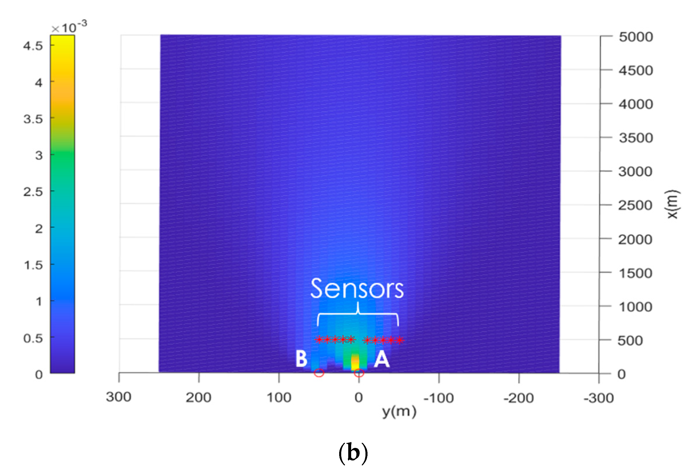
It is assumed that the atmospheric transport and dispersion in the chemical industry park can be described by the Gaussian plume model (1) with the dispersion coefficients a = 0.41455 ,   b = 0.66471 ,   c = 1.00000 ,   and   d = 0.38006 and the meteorological condition that wind speed v = 3 m/s and wind direction is the same as the direction of the x coordinate. Figure 3 shows an illustration of the concentrations of leaking hazardous gas in the area of concern in the chemical industry park over the spatial plane of z = 9 m when the strengths of hazardous gas leakages at locations A and B are Q A = 7.5 ;   Q B = 2.5 with unit g/s.
Clearly, in this case study, N = 10 and S = 2. For multi-sensor data-driven STE model building, M = 1600 sets of noise-corrupted multi-sensor data are collected. These data are generated under different strengths of hazardous gas leakages at locations A and B as shown in Table 2 using the Gaussian plume model (1) where the dispersion coefficients and meteorological condition are as specified above. A uniformly distributed random noise δ U ( 0.05 , 0.05 ) is added on top of the Gaussian plume model that generated concentration data such that C j ( i )   C j ( i ) ( 1 + δ ) , i = 1 , , N ; j = 1 , , M , to simulate the measurement errors induced by the environment and other factors in practice. It is worth noting that, because of the effect of noise, the 100 sets of multi-sensor data in the same hazardous-gas-leaking scenario shown in Table 2 are different. Therefore, the collected M = 1600 sets of multi-sensor data are all different, as expected in practice.
We then applied the proposed multi-sensor data-driven STE approach described in Section 4 to the 1600 sets of multi-sensor data. The details and results obtained in each of the 5 steps of the new STE approach are provided as follows:
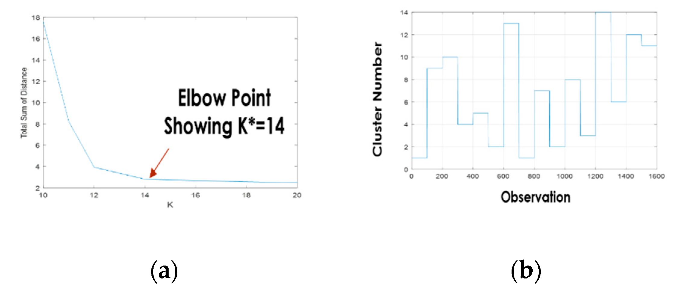
Step 1: Applying K-mean clustering to the M = 1600 measurements from the N = 10 sensors has results shown in Figure 4, indicating that the observed multi-sensor data have K * = 14 clusters. In addition, it can also be found from Figure 4 that Observations i × 100 + 1   to   i × 100 + 100 , i = 0, 1, …, 15 are within the same cluster; Observations 1–100 and 701–800 are in Cluster 1; and Observations 401–500 and 901–1000 are in Cluster 2. Obviously, these results are consistent to the true situation shown in Table 2. The average concentration in each of the 14 clusters, that is, the components in matrix C * , is obtained and shown in Table 3.
Step 2: Applying the analysis in this step to matrix C * shown in Table 3 yields matrices U * and Σ * . Then, by taking ε = 0.02 , it is known from the K * = 14 diagonal entries of Σ * that S ¯ = 2 , that is, there exist 2 hazardous-gas-leaking sources, which is again correct.
Step 3: Applying the analysis in this step to Matrix U * obtained in Step 2 finds p ( 1 ) , ,   p ( S ¯ ) as p ( 1 ) = 4 , p ( 2 ) = 10   and then obtains Matrix C ¯ * , which is composed of the 4th and 10th rows of matrix C ¯ * , that is
C ¯ * ( 1 , : ) = C * ( 4 , : ) = [ 0.006 , 0.0012 , 0.0021 , 0.0031 , 0.0039 , 0.0042 , 0.0037 , 0.0031 , 0.0025 , 0.0021 ]
C ¯ * ( 2 , : ) = C * ( 10 , : ) = [ 0.002 , 0.0004 , 0.0007 , 0.0011 , 0.0015 , 0.0025 , 0.0031 , 0.0037 , 0.0042 , 0.0043 ]
Step 4: The Gaussian plume ATE model (1) is applied offline with a = 0.41455 ,   b = 0.66471 ,   c = 1.00000 ,   and   d = 0.38006 ; v = 3 m/s, and the forward ATD-model-based STE is applied to find the hazardous-gas-leaking location and strength in the two scenarios wherein the N = 10 sensors measurements are C ¯ * ( 1 , : ) (Scenario 1) and C ¯ * ( 2 , : ) (Scenario 2), respectively. The CMA evolution strategy [34] is used to search for an optimal solution to the hazardous-gas-leaking locations and strengths in each case. The results obtained are shown in Table 4.
Consequently, the multi-sensor data-driven STE model (21) is obtained with
[ Q ¯ * 1 ( 1 ) Q ¯ * 1 ( S ¯ ) Q ¯ * S ¯ ( 1 ) Q ¯ * S ¯ ( S ¯ ) ] = [ 7.0180 15.7968 15.5123 5.2388 ]
and
C * = [ 0.006 , 0.0012 , 0.0021 , 0.0031 , 0.0039 , 0.0042 , 0.0037 , 0.0031 , 0.0025 , 0.0021 0.002 , 0.0004 , 0.0007 , 0.0011 , 0.0015 , 0.0025 , 0.0031 , 0.0037 , 0.0042 , 0.0043 ]
Step 5: The multi-sensor data-driven STE model obtained in Step 4 is applied to the real-time measured multi-sensor data in ten different hazardous-gas-leaking scenarios, respectively, to perform the STE in each case. The real hazardous-gas-leaking strength and corresponding multi-sensor data measurements in each of the ten hazardous gas-leaking-scenarios are shown in Table 5. The STE results including the estimated hazardous-gas-leaking strengths and locations in each scenario are also provided in Table 5.
It can be observed from Table 5 that good online STE results have been achieved using the proposed multi-sensor data-driven STE approach. The differences between the true hazardous-gas-leaking strengths ( Q A , Q B ) and locations A :   B : and the estimated results ( Q ^ A , Q ^ B ) and A ^ :   B ^ : are basically due to errors from the offline STE stage in Step 4 when the CMA evolution strategy is used to search for an optimal solution to the hazardous-gas-leaking locations and strengths. This can be improved by using a more effective optimization approach, which is beyond the scope of the present study but will be investigated in future work.
In order to investigate the effects of noise and the number of sensors on the performance of the proposed multi-sensor data-driven STE approach, two additional simulation studies were conducted. In the first additional study, it was assumed that the multi-sensor measurements were noise-free, that is, δ U ( 0 , 0 ) , when multi-sensor data are generated for the simulation study. In the second additional study, only the data from sensors 1, 5, 6, 10 were used to build the multi-sensor data-driven STE model (21) and then use the model to online-process multi-sensor data and perform STE in real time. The results of the two additional studies are shown in Table 6 and Table 7, respectively.
From a comparison of the STE results in Table 5 and Table 6, it can be observed that the results in the noise-free case are slightly better than the results in the case when the multi-sensor data are affected by noise, indicating that the noise does have some effects on the proposed multi-sensor data-driven STE approach but also that the effects are not significant. However, a comparison of the results in Table 5 and Table 7 shows that the number of sensors that can be used to implement the multi-sensor data-driven STE have an obvious impact on the performance of the proposed approach. Basically, the use of more sensors can improve the accuracy of both estimated hazardous-gas-leaking strengths and estimated hazardous-gas-leaking-source locations.

6. Discussion

Current STE approaches are either to online-use ATD-model-based nonlinear optimization to find the locations and strengths of hazardous-gas-leak sources or to rely on a machine-learning-based STE model to associate the field-measured multi-sensor data with the leaking-sources parameters. In the present study, for the first time, the idea of the exploitation of historical multi-sensor observations for the STE of hazardous gas leakages is proposed. The new concept of IHGLSs is introduced, which, under Assumption (6), can fully represent the mechanisms that dominate the hazardous gas leakages in the chemical industrial park of interest. It is shown that the online STE for any hazardous-gas-leak scenario can be achieved using a multi-sensor data-driven STE model derived from the offline STE outcomes and the multi-sensor data collected from these IHGLSs. A further novelty is the innovative data analysis that is introduced to determine the number and the most representative multi-sensor data from these IHGLSs. The results allow the most important historical multi-sensor data to be embedded into a STE model and exploited to carry out online STE. Compared to existing STE methods, the proposed approach has no requirement for ATD-model-based online nonlinear optimization and involves no supervised learning. Therefore, the proposed approach could be more easily adopted and applied in engineering practice. It is worth mentioning that the proposed approach requires that the multi-sensor data used for the multi-sensor data-driven STE model-building cover all the IHGLSs of concern. This condition can be satisfied if a sufficient period of time is used to collect the required historical multi-sensor data. This is because less significant hazardous gas leakages with strengths within allowed limits almost always take place anytime in a chemical industry park, and these routine leaking scenarios are sufficient to cover all of the IHGLSs of concern, provided a sufficient period of time is used for the data collection.

7. Conclusions

Source term estimation (STE) is important for the timely identification of the source of hazardous gas leakages in chemical industrial parks to address environmental pollution and prevent possible accidents. Current STE techniques basically use hazardous gas sensors’ data and rely on running an ATD model online in conjunction with an optimization or Bayesian inference framework to find hazardous-gas-leaking locations and strengths. In addition, many supervised machine-learning-based STE methods have also been proposed to directly associate multi-sensor data with STE outcomes. However, due to complexity and required computation time, the ATD model and online optimization-based STE is difficult to implement in real time. The robustness issue with supervised machine learning implies that machine-learning-based STE is also hard to apply in practice. To address these challenges, a novel multi-sensor data-driven STE approach is proposed in the present study. The approach applies unsupervised multi-sensor data clustering and analysis to historical multi-sensor data collected over a period covering the IHGLSs of concern. This, in conjunction with the offline application of a forward ATD-model-based STE, produces a multi-sensor data-driven STE model that can be directly used to online-process multi-sensor data and conduct STE in real time. In principle, this approach can fundamentally resolve time-consumption-, complexity-, and robustness-related difficulties with existing STE techniques. Simulation studies have verified the effectiveness of the proposed approach. In order to better reveal the main idea, the present study only considers relatively simple scenarios, wherein the Gaussian plume model is used as the ATD model, one meteorological condition is taken into account, and the IHGLSs don’t change with time. Future studies will be focused on more-complicated situations, including hazardous-gas-leakage scenarios represented by high-fidelity CFD models, as well as applying the proposed approach to multi-sensor data from chemical industry parks to carry out STE studies on real industrial scenarios.

Author Contributions

Conceptualization, Z.L.; methodology, Z.L.; software, Z.L. and Y.W.; validation, Y.W.; formal analysis, Z.L.; investigation, Z.L., B.W., Y.W., C.C. and X.P.; resources, W.D. and F.Q.; data curation, Y.W.; writing—original draft preparation, Z.L.; writing—review and editing, Z.L. and B.W.; visualization, Z.L. and Y.W.; supervision, Z.L. and B.W.; project administration, B.W., W.D. and F.Q.; funding acquisition, W.D. and F.Q. All authors have read and agreed to the published version of the manuscript.

Funding

This work was supported by National Natural Science Foundation of China Basic Science Centre Program Grant: 61988101, Key Program Grant: 62136003, and Grant 22178103.

Conflicts of Interest

The authors declare no conflict of interest.

Appendix A

Proof of Proposition 1:
From Assumption (5), the relationship between the strength of hazardous gas leaking and multi-sensor data at any location as shown by a ATD model such as Equation (1) implies that C ¯ j ¯ ( 1 ) , , C ¯ j ¯ ( N ) j ¯ = 1 , , S ¯ are S ¯ linearly independent rows of matrix C. So, Point (ii) is valid.
From Assumption (4) and point (ii), it is known that any row in matrix C can be represented by a linear combination of C ¯ j ¯ ( 1 ) , , C ¯ j ¯ ( N ) j ¯ = 1 , , S ¯ . Therefore, Point (i) is proven.
As C ( 1 ) , , C ( N ) are the multi-sensor data measured in a hazardous-gas-leaking scenario wherein the hazardous gas leakage is generated by the same S ¯ leaking sources, [ C ( 1 ) , , C ( N ) ] T can be represented by a linear combination of C ¯ j ¯ ( 1 ) , , C ¯ j ¯ ( N ) j ¯ = 1 , , S ¯ , that is
[ C ( 1 ) C ( N ) ] = [ C ¯ 1 ( 1 ) C ¯ S ¯ ( 1 ) C ¯ 1 ( N ) C ¯ S ¯ ( N ) ] [ ρ 1 ρ S ¯ ] = C ¯ T [ ρ 1 ρ S ¯ ]
where ρ 1   , ,   ρ S ¯ satisfies
[ Q 1 Q S ¯ ] = [ Q ¯ 1 ( 1 ) Q ¯ 1 ( S ¯ ) Q ¯ S ¯ ( 1 ) Q ¯ S ¯ ( S ¯ ) ]   [ ρ 1 ρ S ¯ ]
Therefore,
[ Q 1 Q S ¯ ] = [ Q ¯ 1 ( 1 ) Q ¯ 1 ( S ¯ ) Q ¯ S ¯ ( 1 ) Q ¯ S ¯ ( S ¯ ) ] ( C ¯ C ¯ T ) 1 C ¯ [ C ( 1 ) C ( N ) ]
that is, Point (iii) is valid. □

References

  1. Wang, B.; Li, D.; Wu, C. Characteristics of hazardous chemical accidents during hot season in China from 1989 to 2019 A statistical investigation. Saf. Sci. 2020, 129, 104788. [Google Scholar] [CrossRef]
  2. Wang, J.; Fan, Y.; Niu, Y. Routes to failure: Analysis of chemical accidents using the HFACS. J. Loss Prev. Process Ind. 2021, 75, 104695. [Google Scholar] [CrossRef]
  3. Tahmid, M.; Dey, S.; Syeda, S.R. Mapping human vulnerability and risk due to chemical accidents. J. Loss Prev. Process Ind. 2020, 68, 104289. [Google Scholar] [CrossRef]
  4. Zhang, Y.; Oldenburg, C.M.; Pan, L. Fast estimation of dense gas dispersion from multiple continuous CO2 surface leakage sources for risk assessment. Int. J. Greenh. Gas Control 2016, 49, 323–329. [Google Scholar] [CrossRef]
  5. Hutchinson, M.; Oh, H.; Chen, W.H. A review of source term estimation methods for atmospheric dispersion events using static or mobile sensors. Inf. Fusion 2017, 36, 130–148. [Google Scholar] [CrossRef]
  6. Keats, A.; Yee, E.; Lien, F.S. Bayesian inference for source determination with applications to a complex urban environment. Atmos. Environ. 2007, 41, 5547–5551. [Google Scholar] [CrossRef]
  7. Xue, F.; Kikumoto, H.; Li, X.; Ooka, R. Bayesian source term estimation of atmospheric releases in urban areas using LES approach. J. Hazard. Mater. 2018, 349, 68–78. [Google Scholar] [CrossRef]
  8. Ryan, S.D.; Arisman, C.J. Uncertainty quantification of steady and transient source term estimation in an urban environment. Environ. Fluid Mech. 2021, 21, 713–740. [Google Scholar] [CrossRef]
  9. Bieringer, P.E.; Young, G.S.; Rodriguez, L.M.; Annunzio, A.J.; Vandenberghe, F.; Haupt, S.E. Paradigms and commonalities in atmospheric source term estimation methods. Atmos. Environ. 2017, 156, 102–112. [Google Scholar] [CrossRef]
  10. Wang, Y.; Huang, H.; Huang, L.; Zhang, X. Source term estimation of hazardous material releases using hybrid genetic algorithm with composite cost functions. Eng. Appl. Artif. Intell. 2018, 75, 102–113. [Google Scholar] [CrossRef]
  11. Li, H.; Zhang, J.; Yi, J. Computational source term estimation of the Gaussian puff dispersion. Soft Comput. 2019, 23, 59–75. [Google Scholar] [CrossRef]
  12. Efthimiou, G.C.; Kovalets, I.V.; Argyropoulos, C.D.; Venetsanos, A.; Andronopoulos, S.; Kakosimos, K.E. Evaluation of an inverse modelling methodology for the prediction of a stationary point pollutant source in complex urban environments. Build. Environ. 2018, 143, 107–119. [Google Scholar] [CrossRef]
  13. Cho, J.; Kim, H.; Gebreselassie, A.L.; Shin, D. Deep neural network and random forest classifier for source tracking of chemical leaks using fence monitoring data. J. Loss Prev. Process Ind. 2018, 56, 548–558. [Google Scholar] [CrossRef]
  14. Xu, J.; Du, W.; Xu, Q.; Dong, J.; Wang, B. Federated learning based atmospheric source term estimation in urban environments. Comput. Chem. Eng. 2021, 155, 107505. [Google Scholar] [CrossRef]
  15. Xu, Q.; Du, W.; Xu, J.; Dong, J. Neural network-based source tracking of chemical leaks with obstacles. Chin. J. Chem. Eng. 2021, 33, 211–220. [Google Scholar] [CrossRef]
  16. Ling, Y.; Yue, Q.; Chai, C.; Shan, Q.; Hei, D.; Jia, W. Nuclear accident source term estimation using Kernel Principal Component Analysis, Particle Swarm Optimization, and Backpropagation Neural Networks. Ann. Nucl. Energy 2019, 136, 107031. [Google Scholar] [CrossRef]
  17. Ling, Y.; Yue, Q.; Huang, T.; Shan, Q.; Hei, D.; Zhang, X.; Jia, W. Multi-nuclide source term estimation method for severe nuclear accidents from sequential gamma dose rate based on a recurrent neural network. J. Hazard. Mater. 2021, 414, 125546. [Google Scholar] [CrossRef]
  18. Ma, D.; Zhang, Z. Contaminant dispersion prediction and source estimation with integrated Gaussian-machine learning network model for point source emission in atmosphere. J. Hazard. Mater. 2016, 311, 237–245. [Google Scholar] [CrossRef]
  19. Kumar, P.; Singh, S.K.; Ngae, P.; Feiz, A.A.; Turbelin, G. Assessment of a CFD model for short-range plume dispersion: Applications to the Fusion Field Trial 2007 (FFT-07) diffusion experiment. Atmos. Res. 2017, 197, 84–93. [Google Scholar] [CrossRef]
  20. Szegedy, C.; Zaremba, W.; Sutskever, I.; Bruna, J.; Erhan, D.; Goodfellow, I.; Fergus, R. Intriguing properties of neural networks. arXiv 2013, arXiv:1312.6199. [Google Scholar]
  21. Rybchuk, A.; Alden, C.B.; Lundquist, J.K.; Rieker, G.B. A Statistical Evaluation of WRF-LES Trace Gas Dispersion Using Project Prairie Grass Measurements. Mon. Weather Rev. 2021, 149, 1619–1633. [Google Scholar] [CrossRef]
  22. Jia, M.; Huang, X.; Ding, K.; Liu, Q.; Zhou, D.; Ding, A. Impact of data assimilation and aerosol radiation interaction on Lagrangian particle dispersion modelling. Atmos. Environ. 2012, 247, 118179. [Google Scholar] [CrossRef]
  23. De Visscher, A. Air Dispersion Modeling: Foundations and Applications; Chapter 6, Section 6.7; Wiley: New York, NY, USA, 2013. [Google Scholar]
  24. Zhou, W.; Zhao, X.; Cheng, K.; Cao, Y.; Yang, S.H.; Chen, J. Source term estimation with deficient sensors: Error analysis and mobile station route design. Process Saf. Environ. Prot. 2021, 154, 97–103. [Google Scholar] [CrossRef]
  25. Seinfeld, J.H.; Pandis, S.N. Atmospheric Chemistry and Physics from Air Pollution to Climate Change, 3rd ed.; Wiley: New York, NY, USA, 2016; p. 1414. [Google Scholar]
  26. Abbasia, A.R.; Mahmoudi, M.R. Application of statistical control charts to discriminate transformer winding defects. Electr. Power Syst. Res. 2021, 191, 106890. [Google Scholar] [CrossRef]
  27. Abbasia, A.R.; Mahmoudi, M.R.; Avazzadeh, Z. Diagnosis and clustering of power transformer winding fault types by crosscorrelation and clustering analysis of FRA results. IET Gener. Transm. Distrib. 2018, 12, 4301–4309. [Google Scholar] [CrossRef]
  28. Abbasia, A.R.; Mahmoudi, M.R.; Arefi, M.M. Transformer Winding Faults Detection Based on Time Series Analysis. IEEE Trans. Instrum. Meas. 2021, 70, 3516210. [Google Scholar] [CrossRef]
  29. Ma, D.; Tan, W.; Zhang, Z.; Hu, J. Parameter identification for continuous point emission source based on Tikhonov regularization method coupled with particle swarm optimization algorithm. J. Hazard. Mater. 2017, 325, 239–250. [Google Scholar] [CrossRef]
  30. Zheng, X.; Chen, Z. Inverse calculation approaches for source determination in hazardous chemical releases. J. Loss Prev. Process Ind. 2011, 24, 293–301. [Google Scholar] [CrossRef]
  31. Newman, M.; Hatfield, K.; Hayworth, J.; Rao, P.S.C.; Stauffer, T. A hybrid method for inverse characterization of subsurface contaminant flux. J. Contam. Hydrol. 2005, 81, 34–62. [Google Scholar] [CrossRef]
  32. Haupt, S.E. A demonstration of coupled receptor/dispersion modelling with a genetic algorithm. Atmos. Environ. 2005, 39, 7181–7189. [Google Scholar] [CrossRef]
  33. Haupt, S.E.; Young, G.S.; Allen, C.T. A genetic algorithm method to assimilate sensor data for a toxic contaminant release. J. Comput. 2007, 2, 85–93. [Google Scholar] [CrossRef]
  34. Hansen, N. The CMA Evolution Strategy: A Comparing Review. StudFuzz 2006, 192, 75–102. [Google Scholar]
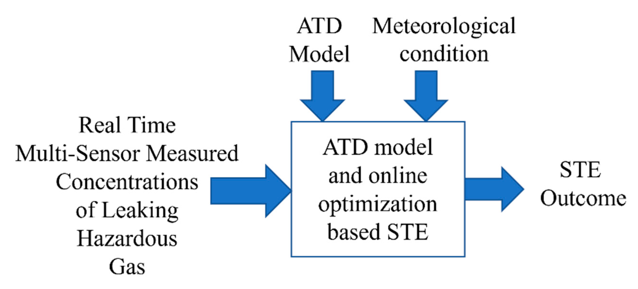
Figure 1. The basic idea of a conventional STE approach.
Processes 10 01633 g001
Figure 2. The novel idea of the proposed multi-sensor data-driven STE.
Processes 10 01633 g002
Figure 3. Concentrations of leaking hazardous gas with unit g/m3 over the spatial plane of z = 9 m when the strengths of hazardous gas leakages are Q A = 7.5   and   Q B = 2.5 with unit g/s. (a) 3D view. (b) Bird’s eye view.
Processes 10 01633 g003aProcesses 10 01633 g003b
Figure 4. The results of multi-sensor data clustering. (a) Total sum of distance (b) Cluster number.
Processes 10 01633 g004
Table 1. The location of hazardous-gas-leaking sources and monitoring sensors.
Leaking
Sources
Leaking Source LocationsSensorsSensor Locations
X0 (m)Y0 (m)Z0 (m)X (m)Y (m)Z(m)
A000Sensor 1
Sensor 2
Sensor 3
Sensor 4
Sensor 5
Sensor 6
Sensor 7
Sensor 8
Sensor 9
Sensor 10
490
490
490
490
490
490
490
490
490
490
−50
−40
−30
−20
−10
10
20
30
40
50
9
9
9
9
9
9
9
9
9
9
B0500
Table 2. Hazardous-Gas-Leaking Scenarios Taken into Account for Multi-Sensor Data-Driven Model Building.
Leaking Scenarios(QA, QB) g/s
1 (observations 1:100)(7.5, 7.5)
2 (observations 101:200)(7.5, 2.5)
3 (observations 201:300)(5, 15)
4 (observations 301:400)(15, 5)
5 (observations 401:500)(10, 10)
6 (observations 501:600)(2.5, 2.5)
7(observations 601:700)(5, 5)
8 (observations 701:800)(7.5, 7.5)
9 (observations 801:900)(1, 1)
10 (observations 901:1000)(2.5, 2.5)
11 (observations 1001:1100)(0, 10)
12 (observations 1101:1200)(10, 0)
13 (observations 1201:1300)(5, 0)
14 (observations 1301:1400)(7, 0)
15 (observations 1401:1500)(7, 1)
16 (observations 1501:1600)(1, 2)
Table 3. Average Concentration in Each Cluster Determined in Step 1.
ClusterAverage Concentration in Each Cluster (g/m3)
10.00030.00060.00100.00160.00200.00250.00250.00250.00250.0024
20.00010.00020.00030.00050.00070.00080.00090.00080.00080.0008
30.00040.00080.00140.00200.00250.00250.00200.00140.00080.0004
40.00060.00120.00210.00310.00390.00420.00370.00310.00250.0020
50.00040.00080.00140.00210.00270.00340.00340.00340.00330.0031
60.00030.00060.00100.00140.00180.00180.00140.00100.00060.0003
70.00000.00010.00010.00020.00030.00030.00030.00030.00030.0003
80.00000.00000.00000.00010.00020.00080.00140.00200.00250.0027
90.00030.00060.00100.00150.00190.00210.00190.00150.00120.0010
100.00020.00040.00070.00110.00150.00250.00310.00370.00420.0043
110.00000.00010.00010.00020.00030.00040.00050.00050.00060.0006
120.00030.00060.00100.00140.00180.00190.00160.00120.00080.0006
130.00020.00040.00070.00100.00140.00170.00170.00170.00170.0016
140.00020.00040.00070.00100.00130.00130.00100.00070.00040.0002
Table 4. Offline STE results obtained in Step 4.
Hazardous-Gas-Leaking ScenariosHazardous-Gas-Leaking Source LocationHazardous-Gas-Leaking Strength g/sEstimated Hazardous-Gas-Leaking-Source LocationEstimated Hazardous-Gas-Leaking Strength g/s
Scenario 1 A : ( 0 , 0 , 0 ) Q A = 5 A ^ : ( 1.4540 , 0.0991 , 0.9282 ) Q ^ A = 7.0180
B : ( 0 , 50 , 0 ) Q B = 15 B ^ : ( 1.5964 , 50.1608 , 0.9200 ) Q ^ B = 15.7968
Scenario 2 A : ( 0 , 0 , 0 ) Q A = 15 A ^ : ( 8.3654 , 0.6043 , 2.4344 ) Q ^ A = 15.5123
B : ( 0 , 50 , 0 ) Q B = 5 B ^ : ( 6.9913 , 52.0679 , 0.0076 ) Q ^ B = 5.2388
Table 5. Online STE results obtained in Step 5.
Hazardous - Gas - Leaking   Strength   ( Q A , Q B )   g / s Corresponding Sensor Data
C = [C(1), C(2), C(3), C(4), C(5), C(6), C(7), C(8), C(9), C(10)] g/m3
Estimated   Hazardous - Gas - Leaking   Strength   ( Q ^ A , Q ^ B )   g / s
(20, 2)[0.00080.00160.00270.00400.00510.00520.00430.00310.00210.0013](20.0762, 2.0618)
(0, 0)[0000000000](0, 0)
(1, 3.5)[0.00000.00010.00010.00020.00030.00050.00070.00080.00100.0010](1.4737, 3.6776)
(22, 17)[0.00090.00180.00310.00450.00590.00700.00680.00640.00610.0055](24.1291, 17.8275)
(4.1, 4.1)[0.00020.00030.00060.00090.00110.00140.00140.00140.00140.0013](4.6256, 4.3020)
(6, 0)[0.00020.00050.00080.00120.00150.00150.00120.00080.00050.0002](5.9399, −0.0123)
(9, 9)[0.00040.00070.00130.00190.00240.00300.00310.00310.00300.0028](10.1537, 9.4435)
(14.14)[0.00060.00110.00190.00290.00380.00470.00470.00470.00470.0044](15.7946, 14.6899)
(13, 1)[0.00050.00100.00180.00260.00330.00340.00280.00200.00130.0008](13.0080, 1.0248)
(1, 12)[0.00000.00010.00020.00030.00050.00120.00180.00260.00310.0033](2.6484, 12.6138)
Hazardous-Gas-Leaking-Source Locations
A : ( 0 , 0 , 0 ) B : ( 0 , 50 , 0 )
Estimated Hazardous-Gas-Leaking-Source Locations
A ^ : ( 4.9097 , 0.3517 , 1.6813 ) B ^ : ( 2.6974 , 51.1144 , 0.562 )
Table 6. Online STE results in the noise-free case.
Hazardous - Gas - Leaking   Strength   ( Q ^ A , Q ^ B )   g / s Estimated   Hazardous - Gas - Leaking   Strength   ( Q ^ A , Q ^ B )   g / s
(20, 2)(19.9965, 1.9479)
(0, 0)(0, 0)
(1, 3.5)(1.4323, 3.4967)
(22, 17)(23.8788, 16.9396)
(4.1, 4.1)(4.5687, 4.0886)
(6, 0)(5.9226, −0.0155)
(9, 9)(10.0288, 8.9749)
(14.14)(15.6003, 13.9609)
(13, 1)(12.9596, 0.9662)
(1, 12)(2.5136, 11.9950)
Hazardous-Gas-Leaking-Source Locations
A : ( 0 , 0 , 0 )
B : ( 0 , 50 , 0 )
Estimated Hazardous-Gas-Leaking-Source Locations
A ^ : ( 3.3933 ,   0.3540 ,   3.3735 )
B ^ : ( 0.9040 ,   51.4910 ,   0.1085 )
Table 7. Online STE results in a case when the data from 4 sensors are used.
Hazardous - Gas - Leaking   Strength   ( Q A , Q B )   g / s Estimated   Hazardous - Gas - Leaking   Strength   ( Q ^ A , Q ^ B )   g / s
(20, 2)(19.9378, 7.3274)
(0, 0)(0, 0)
(1, 3.5)(1.6664, 3.6142)
(22, 17)(24.8458, 22.1976)
(4.1, 4.1)(4.8138, 5.0269)
(6, 0)(5.8632, 1.6251)
(9, 9)(10.5670, 11.0347)
(14.14)(16.4375, 17.1651)
(13, 1)(12.9005, 4.4762)
(1, 12)(3.3401, 11.7337)
Hazardous-Gas-Leaking-Source Locations
A : ( 0 , 0 , 0 )
B : ( 0 , 50 , 0 )
Estimated Hazardous-Gas-Leaking-Source Locations
A ^ : ( 7.6791 ,   3.5176 , 1.6206 )
B ^ : ( 0.1989 ,   52.5589 , 0.9563 )
Publisher’s Note: MDPI stays neutral with regard to jurisdictional claims in published maps and institutional affiliations.