Abstract
Under the dual−carbon goal, the research on energy conservation and emission reduction of new energy vehicles has once again become a current hotspot, and plug−in hybrid electric vehicles (PHEVs) are the first to bear the brunt. In order to improve the fuel economy of PHEV, an adaptive energy management strategy is designed on the basis of the intelligent prediction of driving cycles. Firstly, according to the vehicle dynamics model, the optimal control objective function of PHEV is established, and the relationship between vehicle fuel consumption and driving cycle is analyzed. Secondly, the initial weights and threshold of the backpropagation (BP) neural network are optimized using the particle swarm optimization (PSO) algorithm, and a PSO−BP neural network vehicle velocity prediction controller is established. Thirdly, combined with the approximate equivalent consumption minimization strategy (ECMS) algorithm to calculate the optimal initial equivalent factor in the prediction time domain, the fast−planning SOC and PI control are introduced to determine the optimal equivalent factor sequence, and the optimal torque distribution ratio of the engine and motor is calculated. Lastly, three different energy management strategies are simulated and verified under six China light−duty vehicle test cycle−passenger car (6*CLTC−P) driving cycles. Simulation results show that the established velocity prediction model has good prediction accuracy, and the proposed adaptive energy management strategy based on prediction is 9.85% higher than the rule−based strategy in terms of fuel saving rate and 5.30% higher than the ECMS strategy without prediction, which further improves the fuel saving potential of PHEV.
1. Introduction
While automobiles bring great convenience to the transportation of people and goods, they also further aggravate environmental pollution and energy shortages. In the context of the continuous promotion of energy conservation and emission reduction around the world, the “dual−carbon target” and “new energy automobile industry development plan” promulgated by the Chinese government have accelerated the development of new energy vehicles such as pure electric vehicles (EVs) and plug−in hybrid electric vehicles (PHEVs). In the face of a series of problems such as the short endurance mileage of pure electric vehicles that need to be solved urgently, various large car companies have promoted the development and production of more valuable plug−in hybrid vehicles. Plug−in hybrid electric vehicles take into account the advantages of traditional fuel vehicles and pure electric vehicles. On the one hand, it improves energy utilization efficiency and reduces the emission pollution of traditional fuel vehicles. On the other hand, it has a large−capacity battery, which can be charged externally, taking into account the braking energy recovery function, which alleviates the mileage anxiety of pure electric vehicles and has a very broad development prospect [1,2,3,4,5].
As the core control part of plug−in hybrid electric vehicles, the energy management strategy (EMS) aims to reasonably allocate multiple power sources to improve the vehicle fuel economy under the premise of meeting dynamic performance requirements. This paper analyzes the energy management strategy of new energy vehicles, and strives to achieve driving information prediction, as well as a reduction in the fuel consumption of vehicles, through optimization strategies, so as to alleviate the anxiety of energy shortage. At present, the management strategies of PHEV are mainly divided into two categories. One is the rule−based energy management strategy, and the other is the optimized energy management strategy [6]. The production vehicle mainly adopts the rule−based energy management strategy, such as the charge depleting–charge maintenance (CD−CS) strategy. According to the logical threshold set by the designers, the vehicle operation mode is controlled, and the fuel−saving potential gradually deteriorates with the increase in driving mileage [7]. Since the energy management system of plug−in hybrid electric vehicles is a nonlinear control system with constraints, the optimal control theory was gradually introduced into the study of the energy management problem of PHEV, and the energy management strategy based on global optimization, instantaneous optimization, and intelligent optimization methods was, thus, born. The classical dynamic programming (DP) algorithm [8], Pontryagin’s minimum principle (PMP), equivalent consumption minimization strategy (ECMS) [9], and other methods are used to optimize and improve the control performance of PHEV during operation. DP and other global optimization methods can achieve ideal optimal control effect under fully known driving cycles, but the uncertainty of driving cycles and heavy computational burden make it difficult to achieve online real−time control. At present, they are mainly used to solve the optimal control sequence in an offline state to provide a reference for the design of other energy management strategies including instantaneous optimal control. ECMS based on the PMP principle is a kind of instantaneous optimization strategy that can be used online, which aims to output the control sequence that minimizes the equivalent fuel consumption of the vehicle under the premise of satisfying the dynamic performance. However, the selected equivalent factors are usually not well adapted to the changing actual road conditions, which leads to the failure to achieve the desired control effect.
Driving conditions play an extremely important role in the design and development of energy management strategy. Therefore, the energy management strategy combined with intelligent optimization methods such as driving cycle identification [10], intelligent transportation system [11], and driving cycle prediction [12] came into being. Li [13] used the genetic algorithm optimized k−means clustering algorithm for the identification of driving conditions, and an adaptive energy management strategy combined with the ECMS algorithm was proposed. Simulation results showed that the proposed energy management strategy reduced vehicle fuel consumption by 6.84% compared with the traditional ECMS. Kazemi [14] obtained relevant information from the intelligent transportation system (ITS) to predict driving conditions and traffic flow. On the basis of the above information, an adaptive ECMS that can dynamically adjust the equivalent factor was proposed. The strategy improves the fuel economy of the vehicle by combining the intelligent transportation system with the energy management strategy. Hu [15] used the K−NN algorithm to predict the future driving conditions, thus establishing an online monitoring control strategy is established. Compared with the traditional ECMS strategy, the proposed optimization strategy greatly improved the fuel economy of the vehicle in both standard and actual conditions. The energy management strategy based on condition identification can improve the adaptability of management strategy to driving conditions to a certain extent, so as to improve the fuel economy of the vehicle. However, it relies on historical vehicle velocity information, which will cause large errors when the road condition is unknown, and the fuel−saving potential of PHEV cannot be fully exerted. In view of the shortcomings of energy management strategy under known driving conditions, the slope information, vehicle velocity information, and other short−term future driving conditions can be used for the prediction, in order to further improve the fuel efficiency of the energy management strategy [16]. At present, the prediction methods of driving conditions mainly include index prediction, Markov prediction, and neural network prediction [17]. The index prediction parameters are fixed, which cannot reflect the dynamic change characteristics of the vehicle. Markov chain prediction has random uncertainty, which cannot achieve predictive prediction when the vehicle motion trend changes. When there are a large number of historical working condition data, the short−term future motion trend and driving condition information can be reasonably predicted using a trained neural network. In this paper, a backpropagation neural network (BPNN) with good nonlinear mapping ability and generalization ability is used to predict the future short−term driving conditions to optimize the PHEV energy management strategy and improve the vehicle fuel economy.
A plug−in hybrid vehicle with P2 configuration was selected as the research object of this paper, and the energy management strategy of PHEV based on condition prediction was studied through a co−simulation using Matlab/Simulink and Cruise software.
This paper is structured as follows: Section 1 discusses the research progress of energy management strategies in recent years and the research content of this paper. Section 2 presents the PHEV architecture adopted in this paper and an appropriately simplified model. The optimal control problem of PHEV is analyzed in Section 3, which provides a theoretical basis for the optimization of energy management strategies in the next step. In Section 4, we optimize the weights and thresholds of the BP neural network with the particle swarm optimization algorithm to complete the establishment of the PSO−BP vehicle velocity prediction model. In Section 5, we propose an A−ECMS energy management strategy with the potential for online implementation, with the goal of minimizing the equivalent fuel consumption, combined with vehicle speed prediction. We summarize and analyze the simulation results in Section 6.
2. PHEV Vehicle Modeling
2.1. Vehicle Architecture and Component Parameters
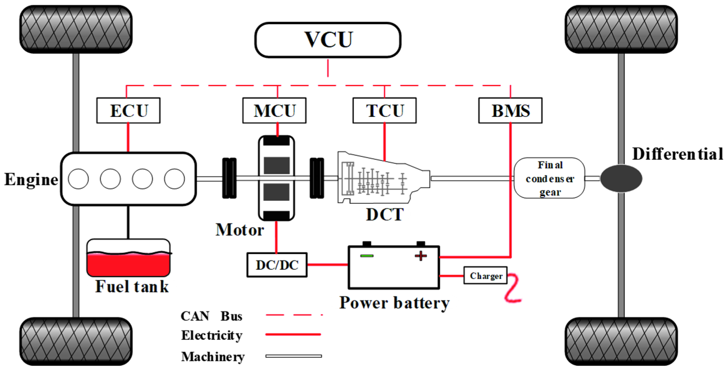
In this paper, the coaxial P2 configuration PHEV is used as the research object, which is mainly composed of an engine, motor, power battery, and transmission system. The engine and ISG motor are arranged in coaxial parallel, and their maximum power is 83 kW and 30 kW, respectively. As shown in Figure 1, during the operation of the vehicle, the engine plays a different role according to the operation state of the vehicle. It can drive the vehicle alone, drive the vehicle at the same time with the motor, or drive the motor to charge the power battery. The key component parameters of the PHEV are shown in Table 1.
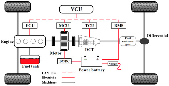
Figure 1.
Parallel plug−in hybrid electric vehicle (PHEV) power system.

Table 1.
Key component parameters.
2.2. Model of Vehicle Dynamics and Key Components
2.2.1. Vehicle Dynamics Model
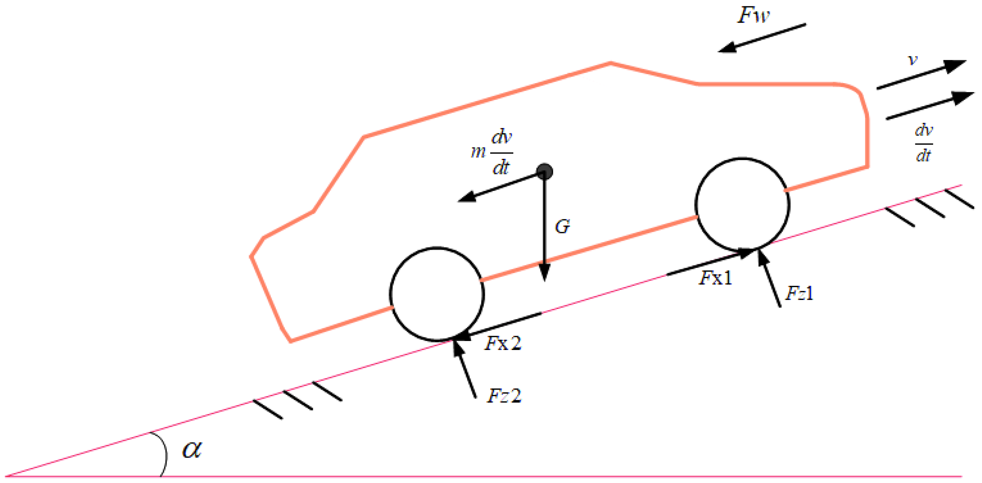
Considering the main research purposes of vehicle power performance and fuel economy in this paper, a simplified vehicle longitudinal dynamic model was established. When the vehicle accelerates uphill at velocity and acceleration , the force analysis is as shown in Figure 2.
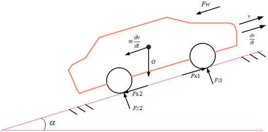
Figure 2.
Force analysis chart of parallel PHEV.
The driving resistance of vehicles can be described as
where is the driving resistance, is the rolling resistance, is the air resistance, is the slope resistance, is the acceleration resistance, , represents the vehicle mass, represents rolling resistance coefficient, represents the air resistance coefficient, represents the windward area, represents the air density, represents the rotation mass conversion coefficient, and represents the velocity. Accordingly, the required torque of the vehicle can be calculated as
where is the rolling radius of the tire.
2.2.2. Engine Model
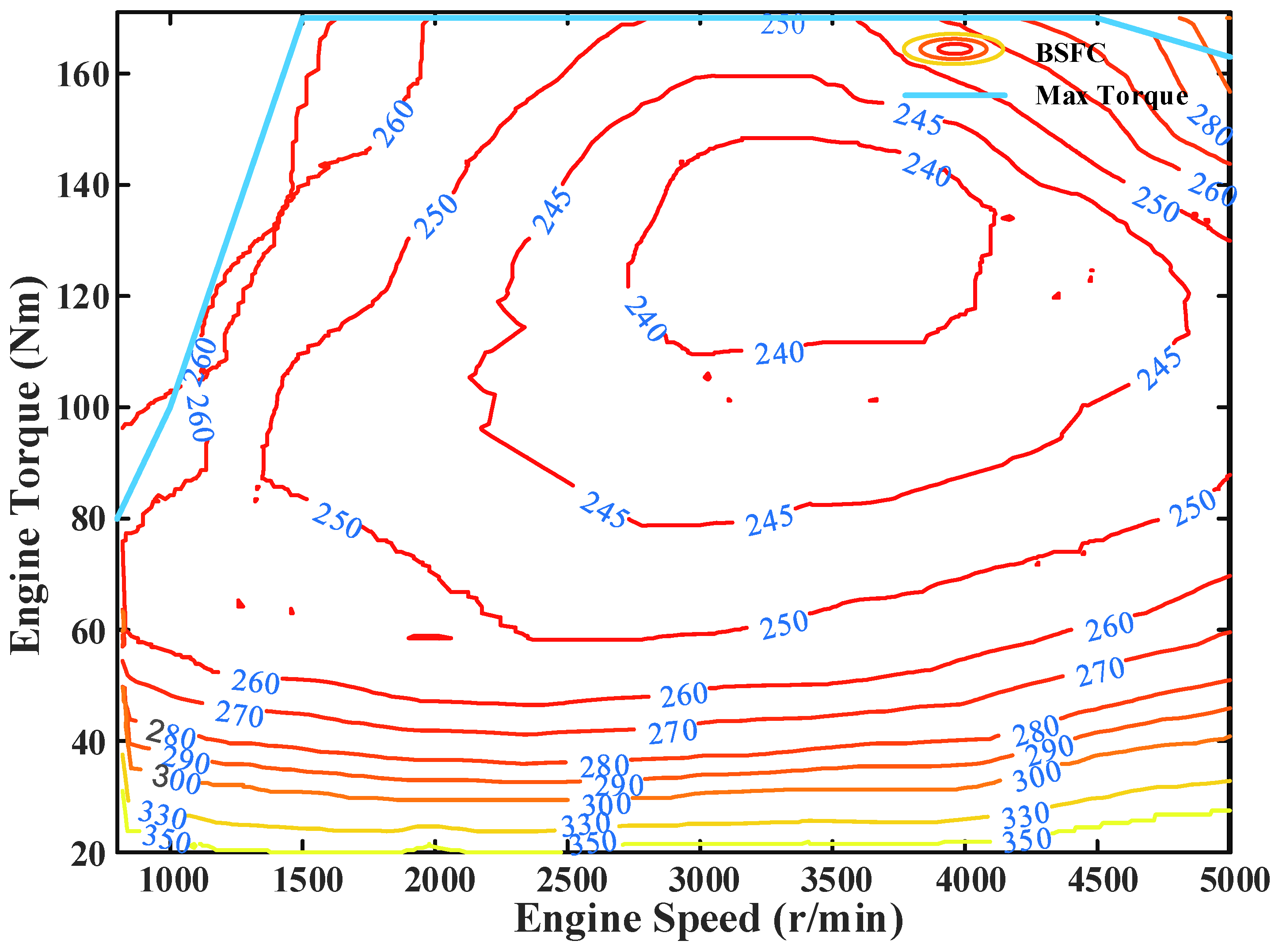
By only considering the fuel consumption characteristics of the engine, the engine model can be appropriately simplified. Here, the static graph modeling method was used to replace the complex modeling. The engine universal characteristic curve is shown in Figure 3. Engine instantaneous fuel consumption can be described as
where and c are the torque and revolution speed corresponding to a certain operation time of the engine.
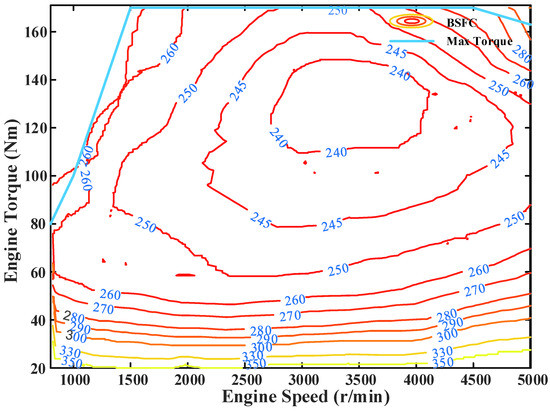
Figure 3.
Universal characteristics of the engine.
2.2.3. Motor Model
The ISG motor used in the drive system can not only provide the required torque of the vehicle as a power source, but also provide charging when the battery power is insufficient. The maximum torque output of the motor during charging and discharging is 140 N·m. For most working areas, the working efficiency of the motor (the efficiency of the inverter is not included here) is maintained between 80% and 90%, and the maximum efficiency is 92%; what needs to be determined is that the efficiency of the inverter is 89%. The motor characteristic diagram shown in Figure 4 was constructed using the experimental data of the motor. The real−time charging and discharging efficiency of the motor was obtained by inputting the motor revolution speed and torque.
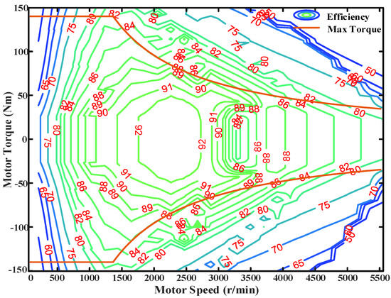
Figure 4.
Motor characteristics.
The power of the motor under different states can be calculated using the following formula:
where is the rotational speed, is the torque, and is the corresponding motor efficiency.
2.2.4. Battery Model
If the thermal temperature effect and transient are ignored, the physical model of the battery can be considered as a static equivalent circuit. According to Kirchhoff’s voltage law, the equivalent circuit equation can be described as
where is the terminal voltage, is the open circuit voltage, is the equivalent internal resistance, and is the current of the battery.
The battery state of charge (SOC) is defined as the ratio of the charge stored in the current battery to the total charge; the change rate of the battery charge state over time can be described as
where is the power of the battery, and is the capacity of the battery.
2.2.5. Transmission Model
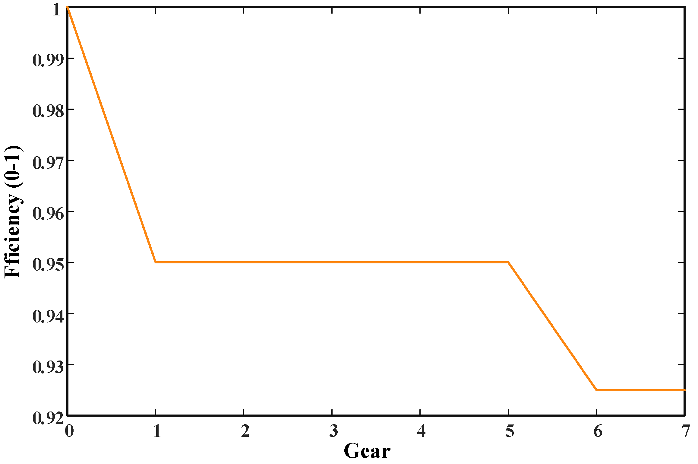
Due to its high transmission efficiency and fuel−saving advantages, dual−clutch gearboxes are favored by domestic and foreign manufacturers and are widely used in hybrid vehicles. A seven−speed dual−clutch gearbox is adopted in this paper to achieve a smooth output of vehicle power and high fuel economy. Figure 5 shows the transmission efficiency of the gearbox in different gears.
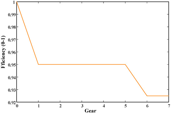
Figure 5.
Transmission efficiency in different gears.
3. Energy Management Optimization Problem
There are many multi−objective optimization problems with constraints in reality, which aim to minimize the cost input under the conditions [18,19]. The energy management optimization problem of PHEV is one of them. It can be described as the process of solving the instantaneous optimal control sequences of the engine and motor to satisfy the minimum optimization objective function and constraints of the vehicle control system [20]. The equivalent fuel consumption is selected as the optimization objective of the control system, with the SOC of the power battery as the state variable and the motor torque as the control variable. The constraint conditions of the optimization objective function are defined as the constraints on the output torque, power range of the engine and motor, power of the battery, SOC, and other parameters. According to the above conditions, PHEV optimal control problem can be described as
where is the optimal control sequence satisfying the constraints, is the time at the end of the trip, is the equivalent fuel consumption, and is the set of physical constraints that the control system needs to meet during vehicle driving. When SOC is taken as the state variable, the constraint set of the above optimization problem can be described as
where is the SOC expectation at the end of the stroke, set to 0.30, is the initial value of the battery SOC, set to 0.70, is the battery power, is the torque of the engine, and is the torque of the motor. According to the description of PMP, the optimal control sequence minimizes the Hamilton function value and minimizes the optimization objective function [21]. After the cooperative state variable is introduced, the Hamilton function can be described as
Introducing cooperative state variables, the global optimization problem of energy management of the vehicle power system can be transformed into instantaneous solving problems with Hamilton functions. At this time, the Hamilton function is equal to the sum of the instantaneous fuel consumption of the engine and another part, which can be understood as the product of the cooperative state variable and the instantaneous change in the SOC of the power battery. By solving the minimum value of the Hamiltonian function at each moment, the torque distribution of the powertrain can be obtained accordingly. According to the above description, the Hamilton function of the PHEV system can be changed to
where is the instantaneous fuel consumption of the engine, is the cooperative state variable at time during driving, and is the system state transition equation, which can be interpreted as the change rate of the power battery SOC over time. In the process of using the PMP control strategy to solve the energy control optimization problem offline, the change range of the cooperative state variable is very small, which can be regarded as a constant.
In order to better solve the PHEV control problem, the cooperative state variable is equivalent to the fuel−electricity equivalent factor in the ECMS, and the instantaneous equivalent fuel consumption rate of the vehicle at time can be described as
where is the fuel consumption equivalent to the instantaneous power of the motor. When the required torque of the whole vehicle is known, according to the relationship among the engine, the motor, and the total required torque, the optimal output torque sequence of the motor is calculated, and the optimal output torque of the engine is obtained.
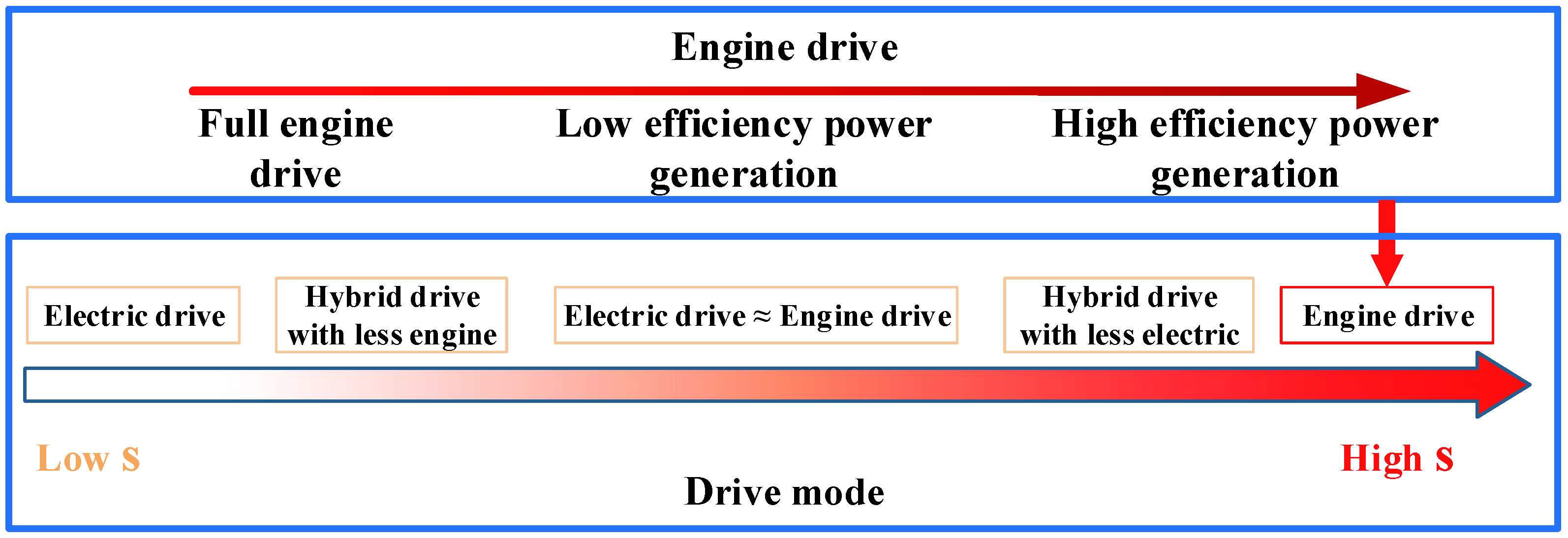
The derivative of the equivalence factor varies so little with time that it is usually constant over the entire travel. Subject to the minimization of the objective function in the ECMS, the fuel economy of the vehicle under different driving cycles is closely related to the selection of the equivalent factor. As shown in Figure 6, as the key parameter for the conversion of fuel and electricity consumption in ECMS, if the equivalent factor is selected too large, the system tends to use more engine drive and increases fuel consumption. On the contrary, if the equivalent factor is too small, it is more inclined to use the motor, reduce the driving power of the engine, and lose the power maintenance [22]. The actual driving road conditions are complex and changeable. How to automatically adjust and change the appropriate equivalent factor according to the driving cycle is an urgent problem to be solved to give full play to the potential of the PHEV’s fuel−saving efficiency.

Figure 6.
Equivalent factorial design logic.
4. Driving Cycle Prediction
The premise of the excellent optimal control effect of the ECMS strategy for the PHEV control system is that the driving cycles are completely known, and the driving cycle information in the future can be predicted using some methods. Information on future driving cycles can be obtained through intelligent transportation systems and predicted by mathematical models. Mathematical model prediction methods such as the exponential function prediction method and neural network prediction method are used to predict future driving cycle information because of their fast and reliable performance [23]. The velocity information involved in this paper is a kind of timeseries information, which has strong nonlinearity and time variability [24,25]. Therefore, the backpropagation neural network with good nonlinear mapping ability and generalization ability was selected for velocity prediction. Lastly, in order to improve the prediction accuracy, the PSO algorithm was used to optimize the BPNN.
4.1. Principle of Neural Network Cycle Prediction
According to the different types of data information, the neural network can conduct the corresponding prediction through the complex learning between multiple neurons. When the type of prediction information is velocity information, assuming and are the input and output of the neural network prediction model, and the prediction step is the step, the model output of the neural network at T time can be described as
A single variable or multiple variables can be used as the input of the neural network velocity prediction model. The common velocity prediction input mainly includes historical velocity information, historical acceleration information, weather information, and traffic information [26]. The trained neural network can predict and continuously adjust the future vehicle velocity according to the selected single or multivariate historical information. Here, the historical velocity information of the past n time steps is selected as the input of the prediction model.
Through the above analysis, the driving cycle prediction principle of the neural network can be described as
where is the mapping function of the selected neural network.
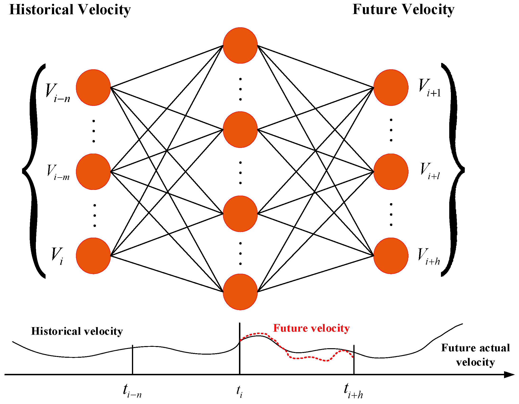
Figure 7 illustrates the principle of using a neural network to predict the vehicle velocity. The established velocity prediction model starts to predict the velocity information of the timestep in the future after having sufficient historical velocity information input. The velocity information is used to solve the optimal equivalent factor by referring to the ECMS until the vehicle reaches the destination.

Figure 7.
Neural network prediction principle diagram.
4.2. Establishment of Comprehensive Driving Cycle
The neural network prediction model needs a large amount of effective velocity sequence information to train to ensure high prediction accuracy. However, the single standard working condition has less data, which cannot reflect the characteristics of the changing working conditions on the actual road. Therefore, it is necessary to establish a representative and large amount of data for the comprehensive driving cycle to train the prediction model.
The characteristic parameters used to describe vehicle driving cycles mainly include average speed, average acceleration, average deceleration, and driving mileage. These parameters are an important basis for dividing different working conditions [27]. In this paper, the maximum speed, maximum acceleration, average acceleration, and average deceleration of driving cycles were determined as the clustering center by clustering identification, which were used as the classification criteria of driving cycles. The 21 standard driving cycles including NEDC, UDDS, NYDC, and US06 were selected to classify and compare similar driving cycles. Table 2 shows the classification results.
Table 2.
Categories of 21 driving cycles and similar conditions.
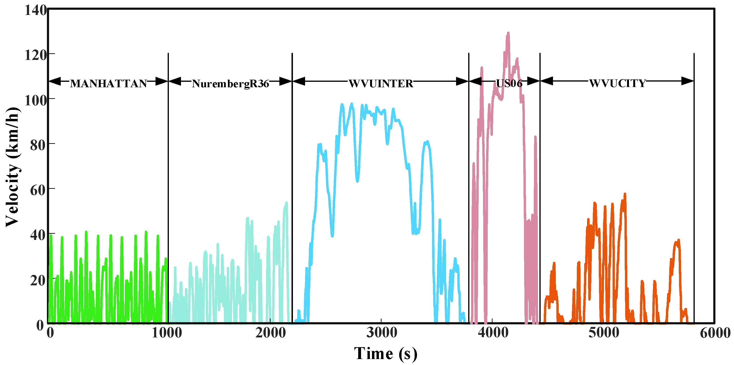
In view of the fact that the vehicle is in the urban condition for a long time in the actual driving process and the road condition is complex and random, this paper selects a cycle in each category and enters the urban condition again after the end of the high−speed condition. Five typical driving cycles (MANHATTAN + NurembergR36 + WVUINTER + US06 + WVUCITY) are finally combined into a representative comprehensive driving cycle. The structure is as follows: congestion condition + urban condition + rapid condition + high−speed condition + urban condition. The established comprehensive driving cycle is used for the training of the neural network predictor to improve its prediction effect. Figure 8 shows the speed–time curve under combined conditions.
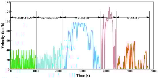
Figure 8.
Comprehensive driving cycles.
The comprehensive driving cycle basically includes all kinds of driving cycles of most people’s daily travel, and it has a certain working condition time guarantee. In theory, the neural network prediction model is trained using the comprehensive driving cycle shown in the above graph, which can ensure that the prediction effect is better in the prediction application process.
4.3. Driving Cycle Prediction Based on PSO−BP Neural Network
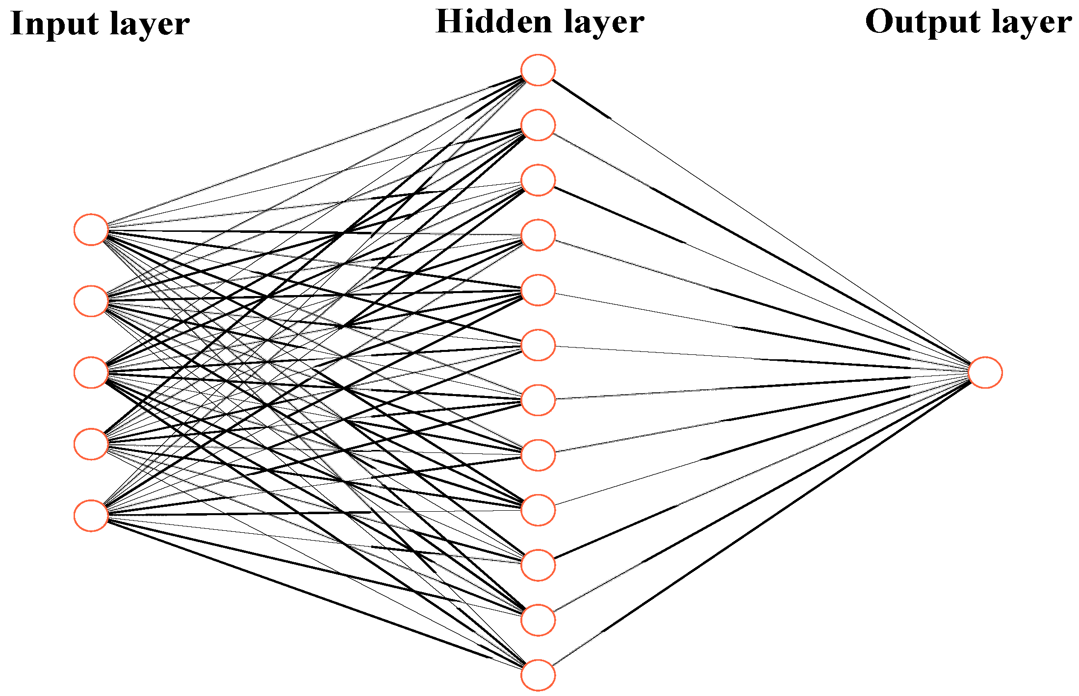
The BP neural network is one of the widely used neural networks with self−learning and adaptive ability. It can realize the minimum error by continuously adjusting the weight of the model, which is mainly used in system model prediction or control. The BP neural network is generally composed of an input layer, hidden layer, and output layer. Each layer contains different numbers of neurons to realize the mutual transmission of information [28,29]. Figure 9 reveals the topological structure of the BP neural network, and the structure of the BP neural network and the number of neurons can be adjusted according to different learning tasks.
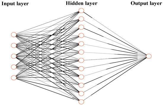
Figure 9.
BP neural network topology.
The original data need to be normalized before network training and testing. In this paper, the comprehensive driving cycle dataset for training was divided into an 80% training set and 20% test set, which was verified by other cycles. After continuous comparative analysis, the velocity information of the past 10 s was determined as the input value of the BP neural network, and the three−layer neural network structure (input layer–hidden layer–output layer) was determined for velocity prediction. There is still no clear formula to solve the optimal number of neural network neurons. In this paper, the number of hidden layer neurons was determined to be 25 through a combination of an empirical formula and the trial−and−error method. The empirical formula of neuron numbers is shown in Equation (17).
where is the number of hidden layer nodes, are the number of input layer and output layer nodes, and is a constant between 1 and 10.
With the continuous development of industrial engineering, the need for process optimization is also increasing. After the advent of the meta−heuristic algorithm, it quickly gained widespread attention and application in the scientific community, and it has solved many industrial engineering problems. Meta−heuristic algorithms are usually inspired by some phenomena in nature, and they achieve the optimal solution in the entire search space while constraining the search process. Common meta−heuristic algorithms mainly include the red deer algorithm (RDA), whale optimization algorithm (WOA), and particle swarm algorithm (PSO). The red deer algorithm is a new evolutionary algorithm inspired by the mating of Scottish red deer in the breeding season, which has high efficiency in solving combinatorial optimization problems [30]. Whales are very intelligent and athletic animals. People got inspiration from the specific hunting behavior of humpback whales and proposed a whale optimization algorithm, which is characterized by improving the rules of candidate solutions in each step of optimization [31]. The particle swarm optimization algorithm is inspired by the predation behavior of birds. It mainly uses the information sharing between each particle to make the movement of the entire particle swarm produce an evolution process from disorder to order in the problem solving space, to obtain the optimal solution to the problem [32,33]. The PSO algorithm is widely used to search for the global optimal solution in the engineering field because of its few parameters and high efficiency. The principle can be described as follows: there is a particle swarm containing N individuals in a D−dimensional search space; each individual is regarded as a particle without volume and weight, which can fly at a certain speed and height in the search space. The flight process is a process to find the optimal solution of the global optimization problem. The m−th particle is represented as a D−dimensional vector , the position of each particle is a potential solution, and the adaptation to measure the pros and cons of the solution can be calculated by bringing into the objective function degree value. The flight speed and group experience in the search process are constantly changing. At time step t, the coordinates and velocity of each generation of particles can be derived from Equations (18) and (19). Assuming as the objective function to be minimized, the current best position of individual m can be determined by Equation (20). The fitness function of PSO is expressed as Equation (21).
where is the inertia weight, which can be calculated using Equation (22), are the learning factors, set to 1.4913, are random numbers between 0 and 1, and are the optimal position of the m−th particle in the historical space and the optimal position of the global particle in the historical space, , and are the corresponding actual output value and expected output value, and the spatial dimension can be determined from the structure of Equation (23) and the BP neural network.
where is the maximum value of inertia weight, with a value of 0.9, whereas is the minimum value of inertia weight, with a value of 0.4. is the current number of iterations, and is the maximum number of iterations set.
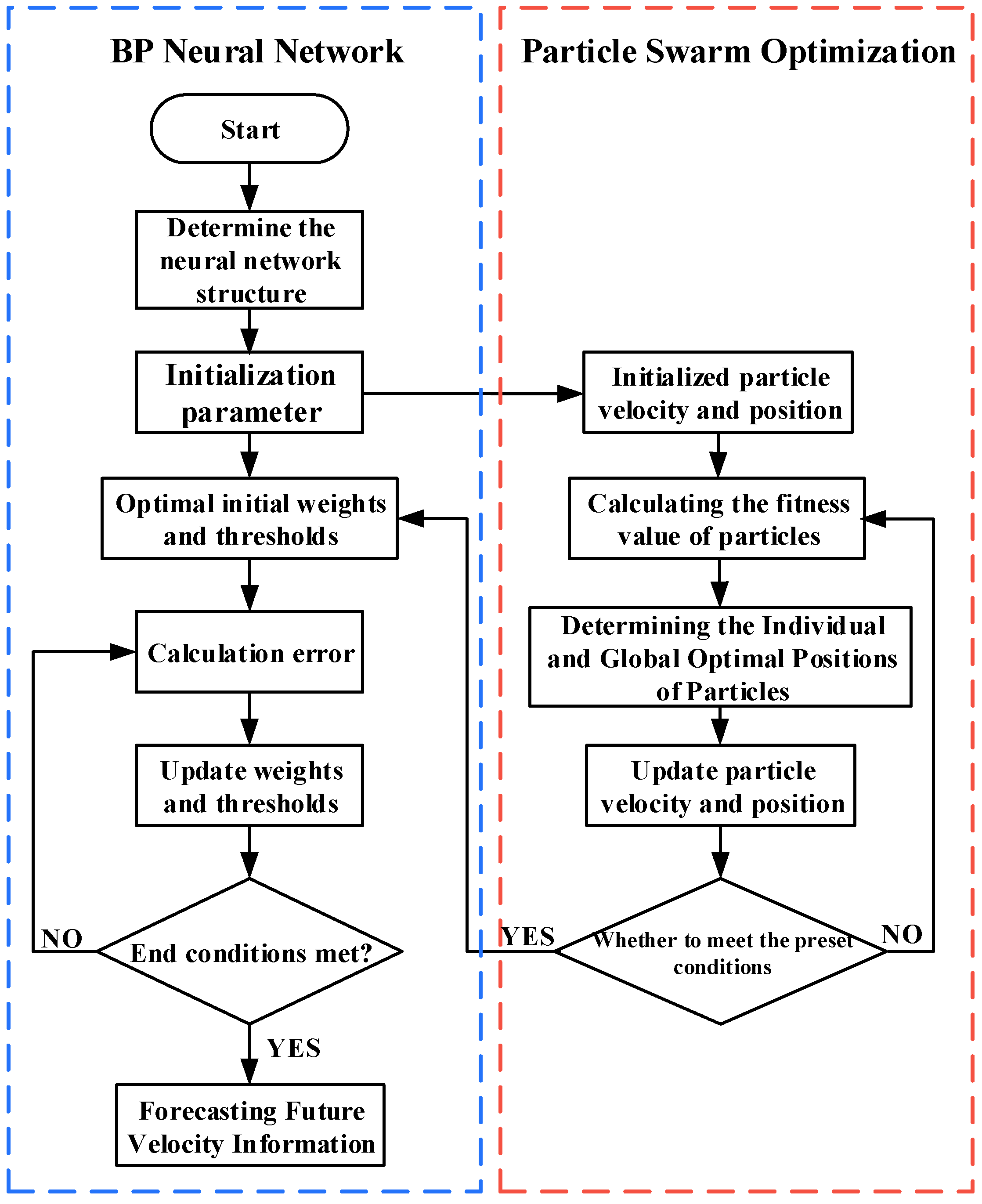
The BP neural network has the advantages of a simple structure and strong adaptability, but some inherent disadvantages such as slow convergence and easy overfitting also exist. The nonlinear error function of BP algorithm is prone to settling in a local minimum in the process of solving, and it is difficult to jump out of the local minimum to find the global optimal solution. The PSO algorithm can search for the optimal solution in a large range, but the calculation accuracy is low, which is the advantage of the BP neural network. In this paper, the PSO algorithm was used to optimize the BP neural network, treating the weights and thresholds of the BP neural network as particles, and a large−scale global search within the scope was carried out to avoid the BP neural network falling into a local maximum, so as to improve the operation efficiency and prediction accuracy of the BP neural network [34].
In the vehicle velocity prediction model based on the PSO−BP algorithm, only the particle swarm algorithm is used to output the optimal initial weights and thresholds of the BP neural network through iterative optimization, while the structure of BP neural network is not changed. The output of the function can be predicted using the trained BP neural network. Figure 10 reveals the flowchart of vehicle velocity prediction based on the PSO−BP algorithm.
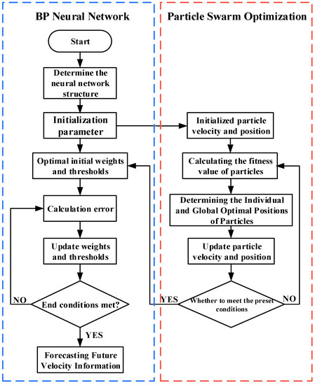
Figure 10.
Flowchart of PSO−BP neural network velocity prediction algorithm.
Many standards have been used to evaluate the performance of prediction models. In this paper, the root−mean−square error (RMSE) was used to evaluate the prediction accuracy of the prediction model in the time domain, which can be defined as
where represents the number of samples, is the predicted velocity, and is the actual velocity. A smaller RMSE indicates a higher prediction accuracy, i.e., the predicted velocity is close to the actual velocity.
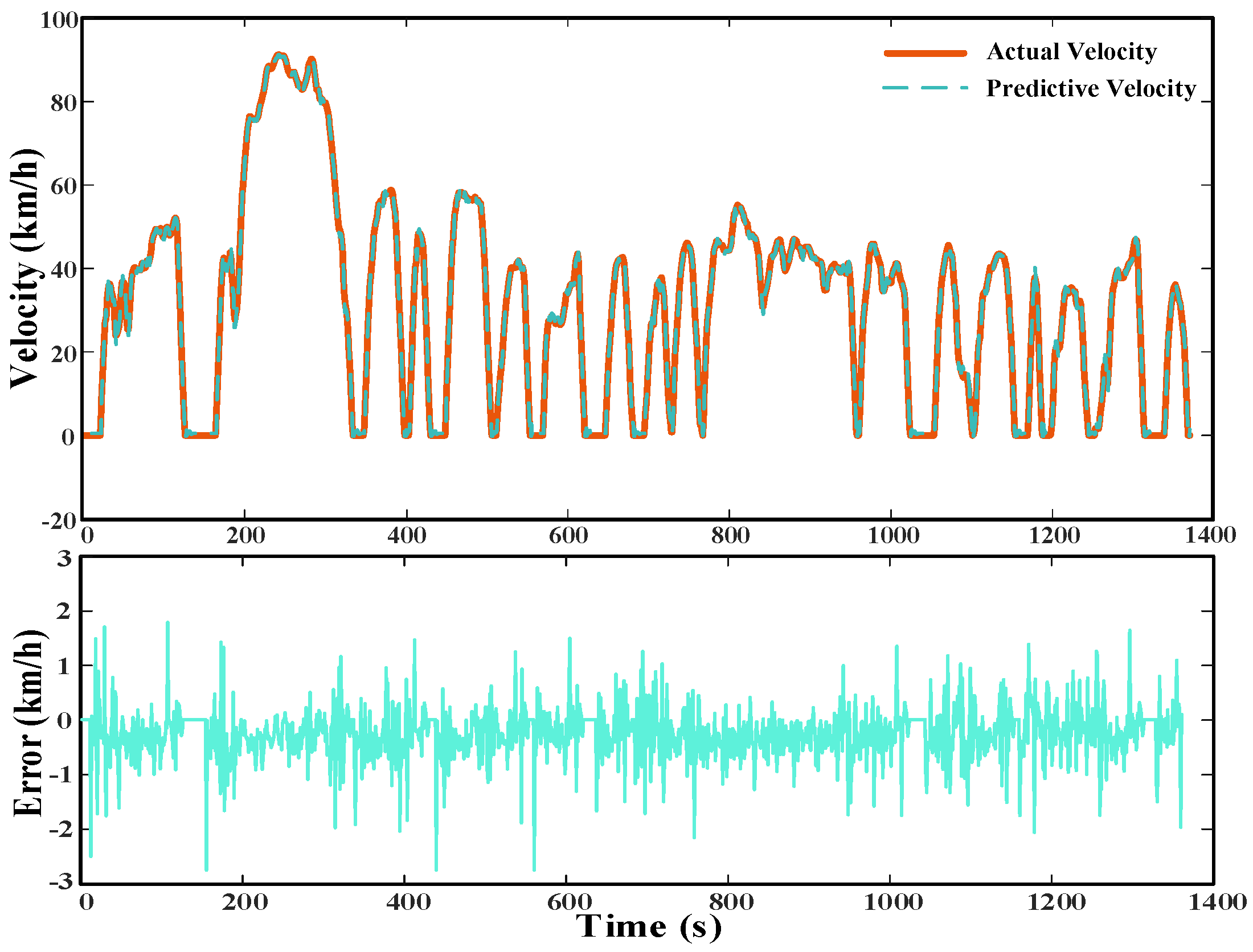
According to the above process, the PSO−BP neural network velocity prediction model was established, and then the urban dynamometer driving schedule (UDDS) standard driving cycle was determined to verify the prediction effect of the model. Figure 11 shows the single−step prediction effect of the prediction model. It can be seen that the predicted velocity followed the actual velocity well. The single−step prediction error was more concentrated within 1 km/h, and the maximum error was also within 3 km/h, thus meeting the accuracy requirements of the prediction. Thus, this approach can be used for multistep prediction.
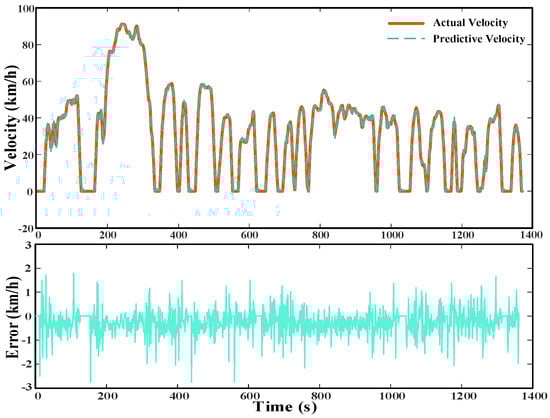
Figure 11.
Single−step prediction effect and error of prediction model under UDDS cycle.
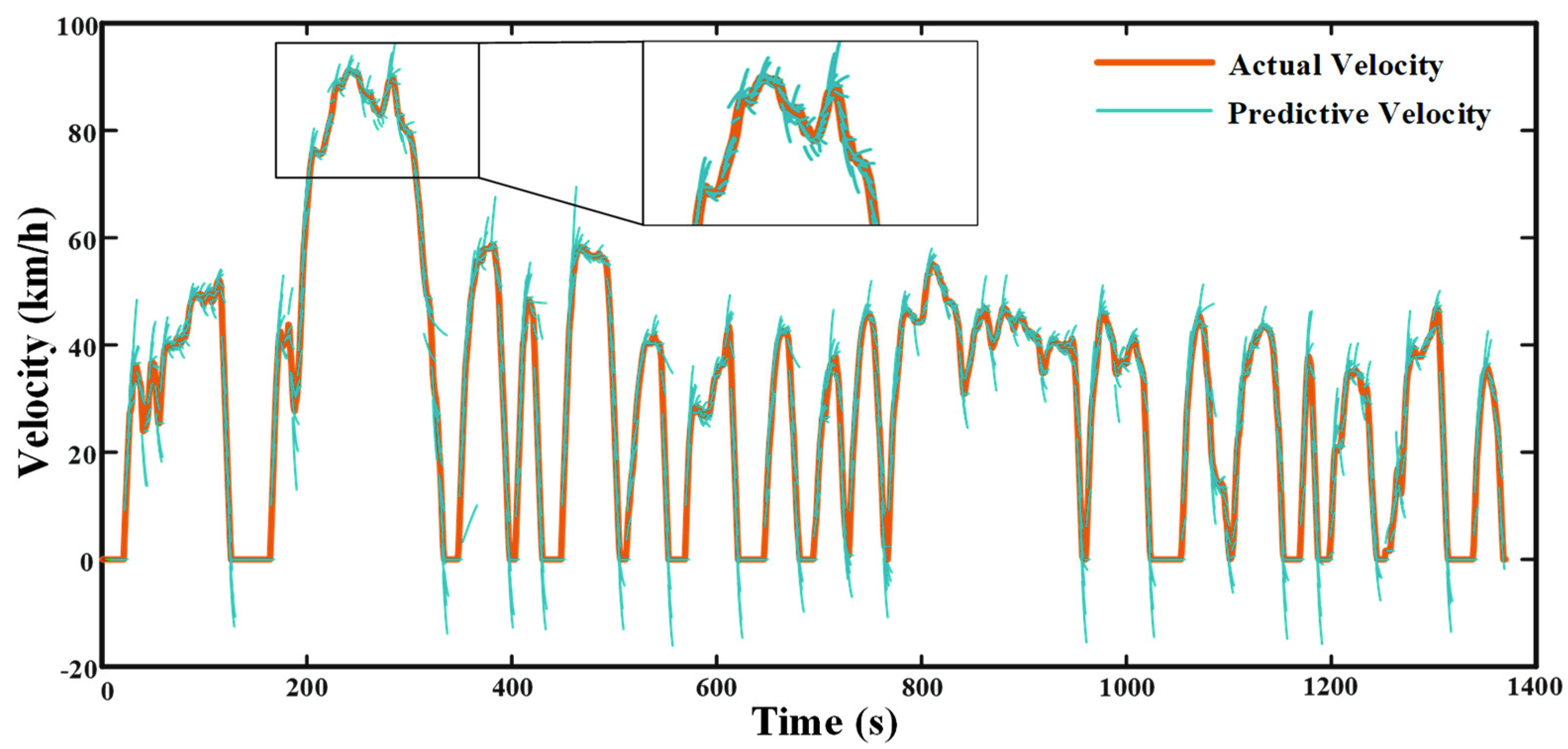
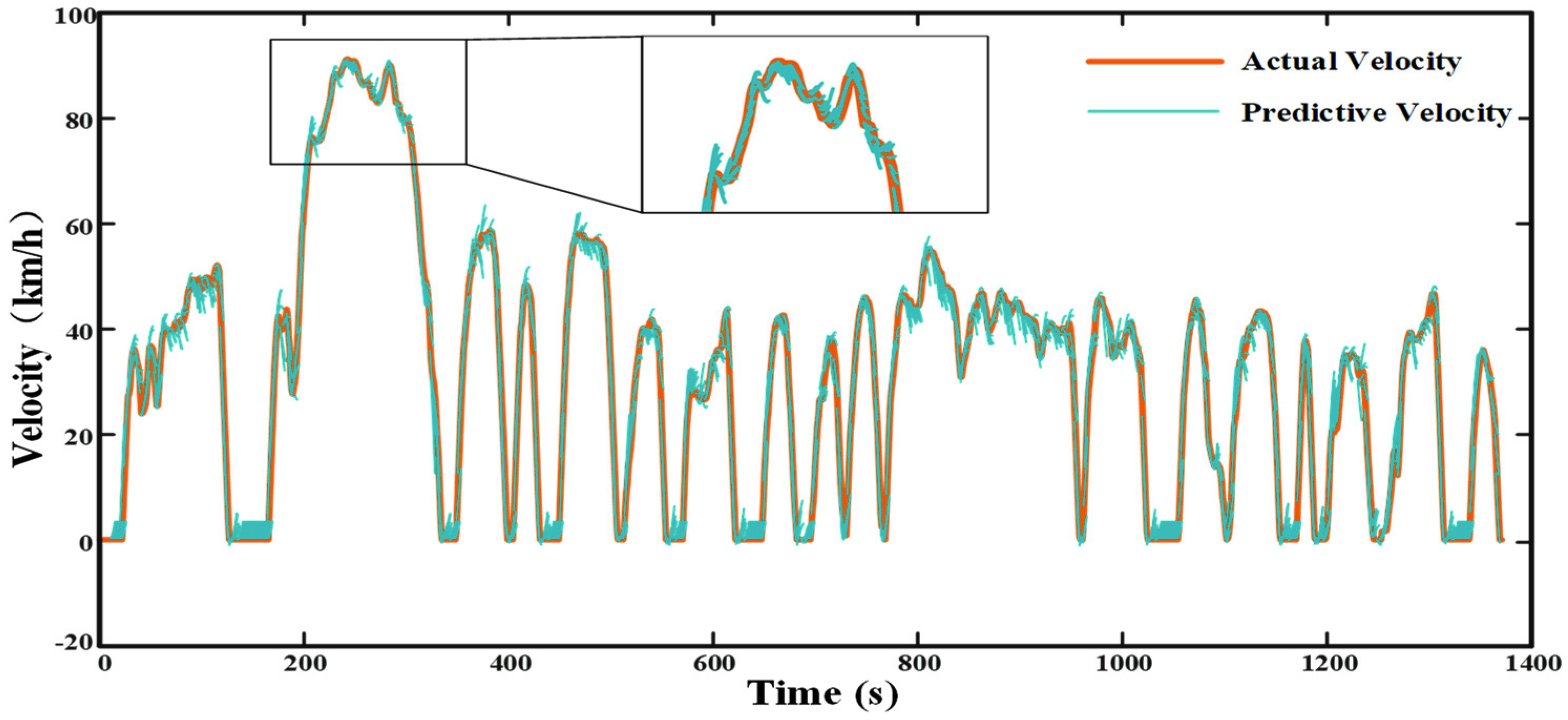
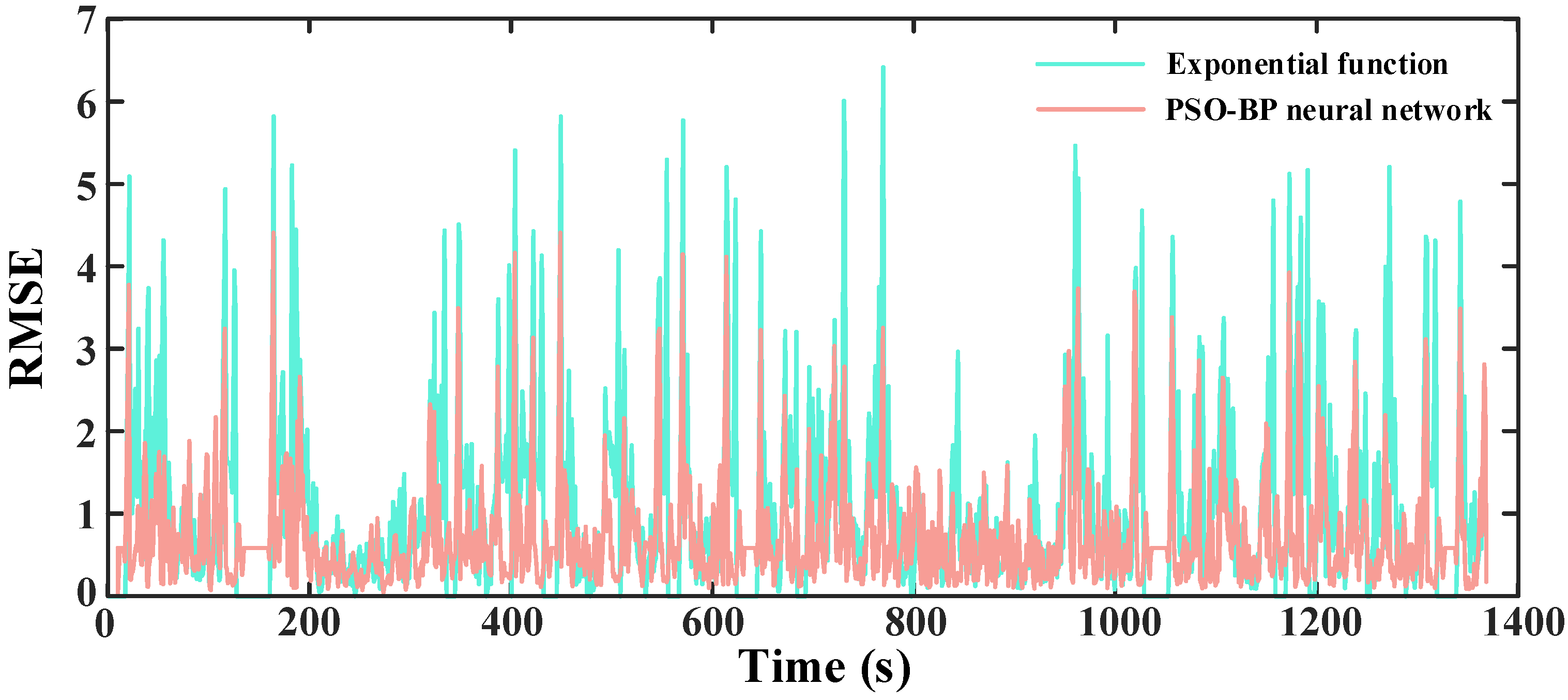
Table 3 reflects the RMSE for different prediction lengths from 3 s to 9 s. It can be seen that the RMSE value for a prediction length of 5 s was 1.4437 km/h, and the error between the prediction velocity and the real value was relatively small, theoretically meeting the usage requirements. As the prediction length increased, the overall fuel consumption of the vehicle showed a small overall fluctuating decrease, but increasing the prediction length, on the other hand, also led to the RMSE value rising significantly and the accuracy of the prediction decreasing, while putting a heavy computational burden on the processor. On the basis of a comprehensive consideration of fuel consumption and computational burden, this paper selected 5 s as the final prediction length for short−term velocity prediction, which was used for the optimization of the energy management strategy below. Figure 12 and Figure 13 show the effect of the exponential prediction and the PSO−BP neural network prediction model on the prediction of vehicle velocity for the next 5 s under the UDDS cycle. It is clear from the figures that the prediction effect under the exponential prediction model was relatively simple, generating a large error in the prediction information at some timepoints where acceleration and deceleration transitions occurred, while it could not predict changes in future driving states. In contrast, the PSO−BP neural network prediction model could reasonably predict vehicle velocity through extensive data learning and nonlinear mapping between neurons, showing good trend prediction compared to exponential prediction [35,36]. We can see from Figure 14 that the RMSE of the exponential prediction model was mostly scattered between 0 and 4 km/h with poor prediction accuracy, while the RMSE values of the PSO−BP neural network prediction model were mainly distributed within 0–2 km/h, and the RMSE value for the whole trip was 1.4437 km/h. This indicates that the PSO−BP neural network vehicle velocity prediction model used in this paper had a better prediction effect, indicating its feasibility to be used for short−term velocity prediction.
Table 3.
Prediction errors of different prediction durations.
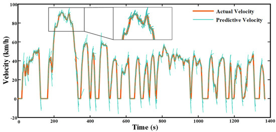
Figure 12.
Prediction performance of exponential predictor at 5 s prediction step.
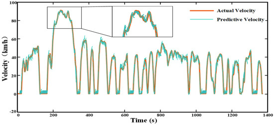
Figure 13.
Prediction performance of PSO−BP neural network predictor at 5 s prediction step.
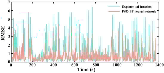
Figure 14.
Root−mean−square error of exponential prediction and PSO−BP neural network prediction.
5. A−ECMS Energy Management Strategy Based on Driving Cycle Prediction
5.1. Adaptive Equivalent Fuel Consumption Minimization Strategy Framework
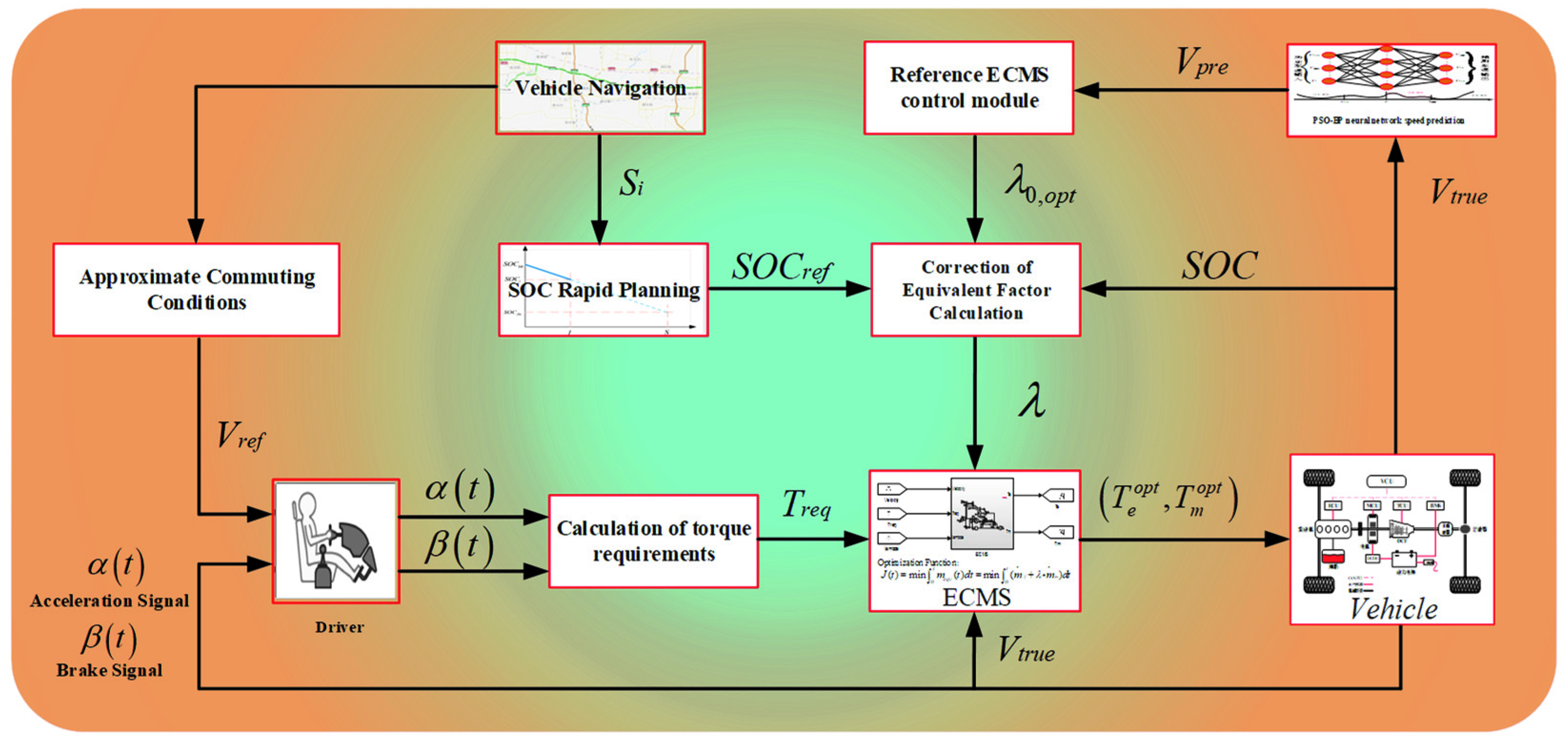
The minimum equivalent fuel consumption strategy is an instantaneous optimization strategy, and the optimization effect depends on whether the selection of the equivalent factor of the key parameter is appropriate. The optimal equivalent factor under one driving cycle may be suboptimal under other driving cycles. In order to further improve the adaptability of energy management strategy to actual road conditions, an adaptive equivalent fuel consumption minimization strategy based on driving cycle prediction is proposed in this paper. Before the start of the trip, the driving mileage is determined according to the navigation, and the reference SOC of the whole trip is reasonably planned. At the same time, the historical commuter driving cycle is used as the reference velocity input of the driver, and the required torque is calculated. The ECMS algorithm is used to solve the power source torque distribution. Then, after reaching the historical velocity information required by the prediction module, the future short−term velocity prediction is carried out, which is input to the reference ECMS control module to solve the initial optimal equivalent factor sequence in the short term in the future. Finally, the modified optimal equivalent factor sequence is applied to the real−time calculation of ECMS in the future prediction time domain, and the optimal power source torque distribution is applied to vehicle control to achieve the purpose of improving vehicle fuel economy.
Figure 15 illustrates the calculation process of the A−ECMS energy management strategy based on driving cycle prediction, where is the predicted velocity, is the actual velocity, is the commuting mileage, is the equivalent factor, and is the time−varying optimal initial equivalent factor obtained according to the prediction.
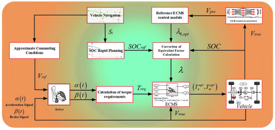
Figure 15.
Flowchart of A−ECMS energy management strategy based on driving cycle prediction.
5.2. Approximate ECMS Algorithm
As shown in Figure 15, after the historical vehicle velocity information is obtained, the PSO−BP neural network predictor predicts the vehicle velocity information in the next 5 s, and the predicted vehicle velocity information is input to the reference ECMS control module to obtain the initial optimal equivalent factor sequence. This module includes a backward vehicle model and an approximate ECMS algorithm, in which the parameters in the backward vehicle model are consistent with the vehicle model established above, except that the predicted vehicle velocity is used as the direct input of the vehicle, and the driver model is cancelled. Combined with the approximate ECMS algorithm, the calculation of the minimum fuel consumption in the predicted time domain and the selection of the optimal equivalent factor can be carried out, but the output of the model does not directly control and change the operating state of the vehicle components.
The approximate ECMS algorithm proposed in this paper was simplified and optimized on the basis of the above ECMS algorithm; the function was unchanged, and the calculation amount was smaller. The principle was to combine the minimum equivalent fuel consumption with the vehicle driving mode switching of the backward vehicle model. First, the driving mode that meets the conditions is selected, and then the instantaneous equivalent fuel consumption and the SOC change value of the battery of the initial equivalent factor are calculated for different numbers in the determined driving mode. is sorted corresponding to the initial equivalent factor satisfying the condition , and the initial equivalent factor with the minimum is determined by performing curve fitting as the optimal initial equivalent factor at time in the future. Next, continuous calculation and optimization are carried out in the entire prediction time domain, and the optimal initial equivalent factor sequence that acts on the ECMS optimization of each step size in the prediction time domain is finally calculated.
The established PHEV working mode is mainly divided into driving main mode, braking main mode, and parking main mode. In the backward vehicle model, the driving main mode is mainly considered, and other modes and related conditions including brake recovery and parking charging are not changed. The main driving mode is further divided into low−speed pure electric driving mode, engine driving mode, charging driving mode, and combined driving mode. The instantaneous equivalent fuel consumption in driving mode can be described as
where is the battery power, is the equivalent factor with a number, refers to the low calorific value of fuel in J/g, and .
The calculation formula of instantaneous equivalent fuel consumption under different driving modes is different, which is mainly due to the different working conditions of the engine and the motor.
- (1)
- Low−speed pure electric driving mode. The switching condition of low−velocity pure electric drive mode is that the vehicle demand torque is less than the maximum torque of the motor, the SOC of the battery is greater than the set minimum SOC limit, and the engine running time is greater than 5 s. In the low−velocity pure electric drive mode, the engine does not work, the value of is set to 0, and the motor torque is greater than zero, providing the driving demand torque of the vehicle.
- (2)
- Engine driving mode. The switching limit of the engine driving mode is that the SOC of the power battery is less than the set minimum value, the vehicle demand torque is greater than the maximum driving torque of the motor, the vehicle demand torque is less than the maximum engine torque, and the running time is less than 5 s. If one of the above conditions is satisfied, the mode can be switched. In the engine driving mode, when the motor does not work, the instantaneous equivalent fuel consumption is the instantaneous fuel consumption of the engine.
- (3)
- Charging driving mode. The switching limit of the driving mode is that the battery SOC is less than or equal to the set minimum SOC limit or the vehicle demand torque is less than the optimal torque of the engine to ensure that the engine can output power for battery charging. Under the charging driving mode, the engine works in the optimal region, i.e., the engine torque is equal to the economically optimal torque in the universal characteristic diagram. At this time, the motor torque and battery power are both negative, and the motor torque value is equal to the difference between the vehicle demand torque and the optimal engine torque.
- (4)
- Combined driving mode. The switching limit of the combined driving mode is that the SOC of the power battery is greater than the minimum SOC limit, and the torque provided by the engine cannot meet the torque demand of the vehicle. At this time, the motor is required to be driven by the combined engine. In the combined driving mode, the engine is still working on the economic optimal curve. The output torque of the motor is the difference between the vehicle demand torque and the optimal torque of the engine. Unlike the charging driving mode, the motor torque and battery power are positive.
In order to reduce the amount of computation in the ECMS reference module, the optimal initial equivalence factor must be found quickly and efficiently, and the selection of the initial equivalence factor can be performed within the following range [37]:
where is the average efficiency of the motor, is the average efficiency of the inverter, is the average efficiency of the battery, and is the average efficiency of the engine.
Within the above range, n equivalent factors are selected at equal intervals and numbered separately, where n is generally defined as 10 and above. Taking the predicted driving speed information as the input, the instantaneous equivalent fuel consumption is calculated in the backward vehicle model according to the determined driving mode, and then the minimum and the corresponding equivalent factor in each calculation are determined. The data are fitted, and the corresponding to the minimum value in the fitted curve is selected as the output of the reference ECMS module, i.e., the initial optimal equivalent factor .
5.3. Reference SOC
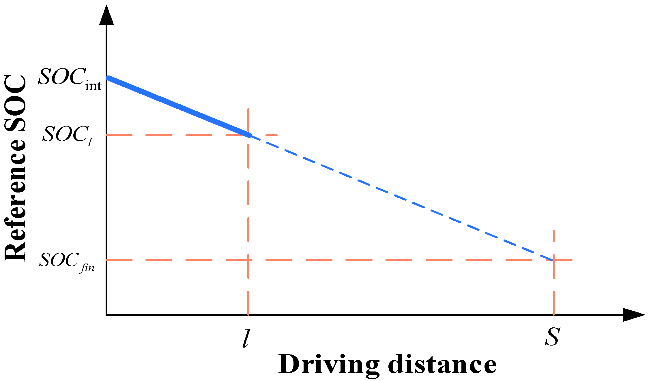
In order to make full use of the fuel−saving performance of PHEV, it is necessary to ensure that the battery power is fully utilized during the entire trip, and the power is only reduced to the set the minimum limit at the end of the planned trip. Therefore, it is necessary to quickly plan the SOC to provide a reference for the actual SOC decline. Studies have shown that the optimal SOC decline trajectory of PHEVs has a linear decreasing relationship with the total travel. When the total travel is greater than the pure electric cruising range of the vehicle, the relationship between the reference SOC trajectory and the driving range can be determined using Equation (27) [38]. Figure 16 shows the planning principle of the reference SOC. Here, the initial value of SOC was determined to be 0.70, and the minimum limit was 0.30.
where is the actual driving distance at time , is the reference SOC corresponding to time , and are the initial SOC value and the final value, and is the total stroke.
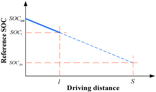
Figure 16.
Reference to SOC planning principle.
In order to ensure that the SOC of the power battery can closely follow the planned reference SOC decline trajectory during the actual driving process, so as to reasonably utilize the power of the power battery and improve the fuel economy of the vehicle, the equivalent factor is dynamically calculated according to the difference between the SOC and the reference SOC. When the difference is positive, it indicates that the battery SOC is less than the planned SOC, and the battery is too low; hence, the equivalent factor needs to be increased. Otherwise, the equivalent factor needs to be decreased. Finally, the equivalent factor is determined as the control variable, the deviation between the actual SOC and the reference SOC is used as the correction, and the PI controller is introduced to solve the optimal equivalent factor in real time.
where and are the proportional and integral parameters of PI controller.
So far, the driving cycle prediction module, reference ECMS module, equivalent factor correction module, and ECMS algorithm have been combined to establish an adaptive equivalent fuel consumption minimum energy management strategy based on driving cycle prediction.
6. Simulation Results and Analysis
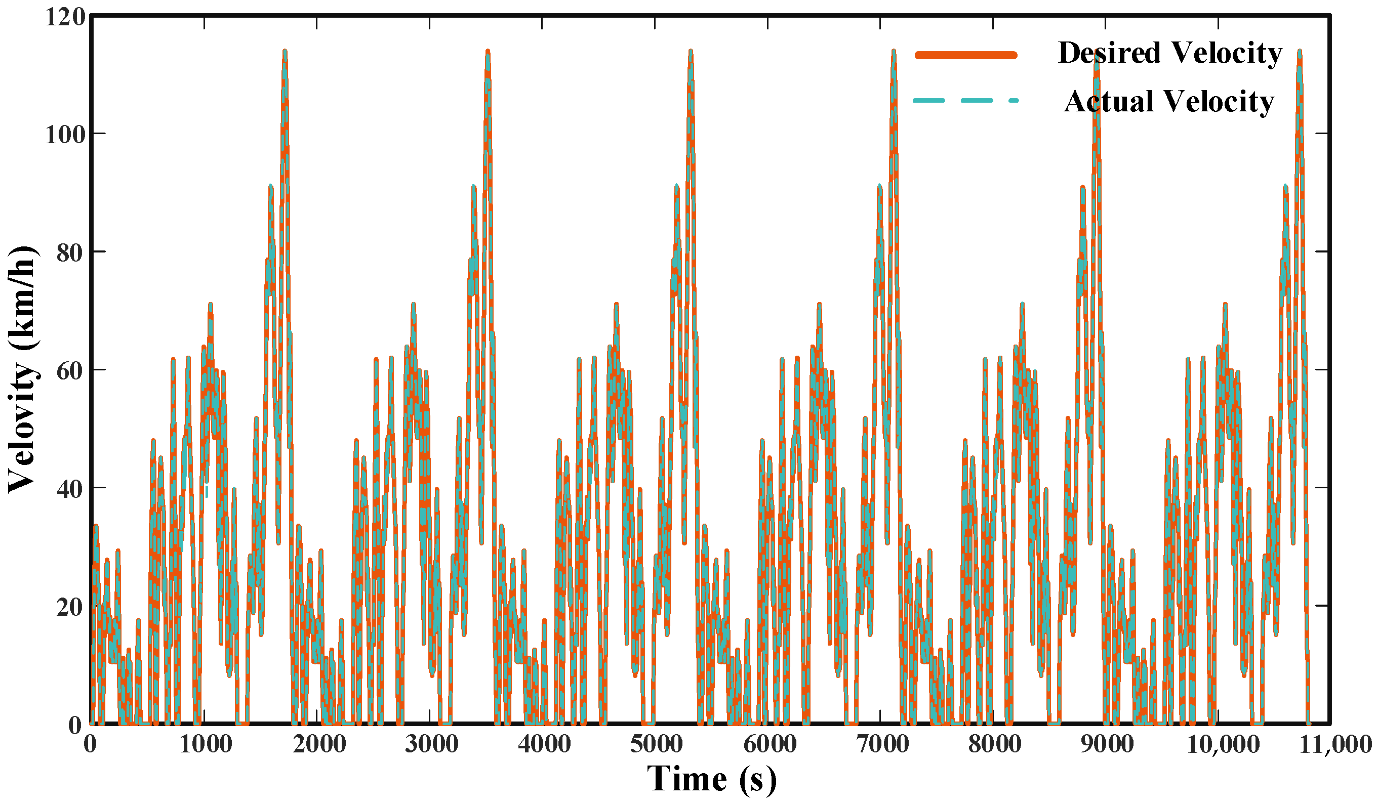
The China light−duty vehicle test cycle−passenger car (CLTC−P) is the light−duty vehicle driving condition independently established by China. It was developed on the basis of vehicle driving data of 5050 vehicles in 41 representative cities across the country with a total of 55 million kilometers. Compared with other typical driving conditions, the cycle is more in line with the actual road driving cycle in our country, such that the energy consumption and emissions of the vehicle laboratory certification are closer to the actual level [39]. Under six China light−duty vehicle test cycle−passenger car (6*CLTC−P) driving cycles, the proposed energy management strategy based on driving cycle prediction was compared with the typical rule−based and ECMS−based energy management strategies to evaluate the optimization effect of the proposed adaptive energy management strategy. Figure 17 shows the velocity–time curve under the 6*CLTC−P cycles and the velocity−following curve of the PHEV during the simulation. It can be seen that the established PHEV vehicle model could meet the dynamic requirements of the vehicle and follow the established cyclic driving cycles well.
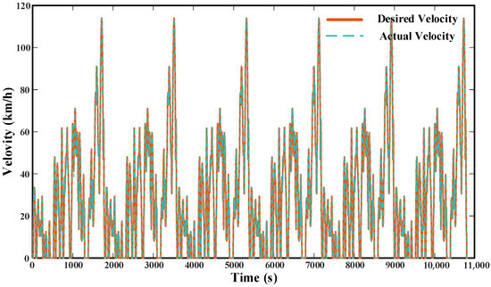
Figure 17.
6*CLTC−P driving cycle and velocity−following curve.
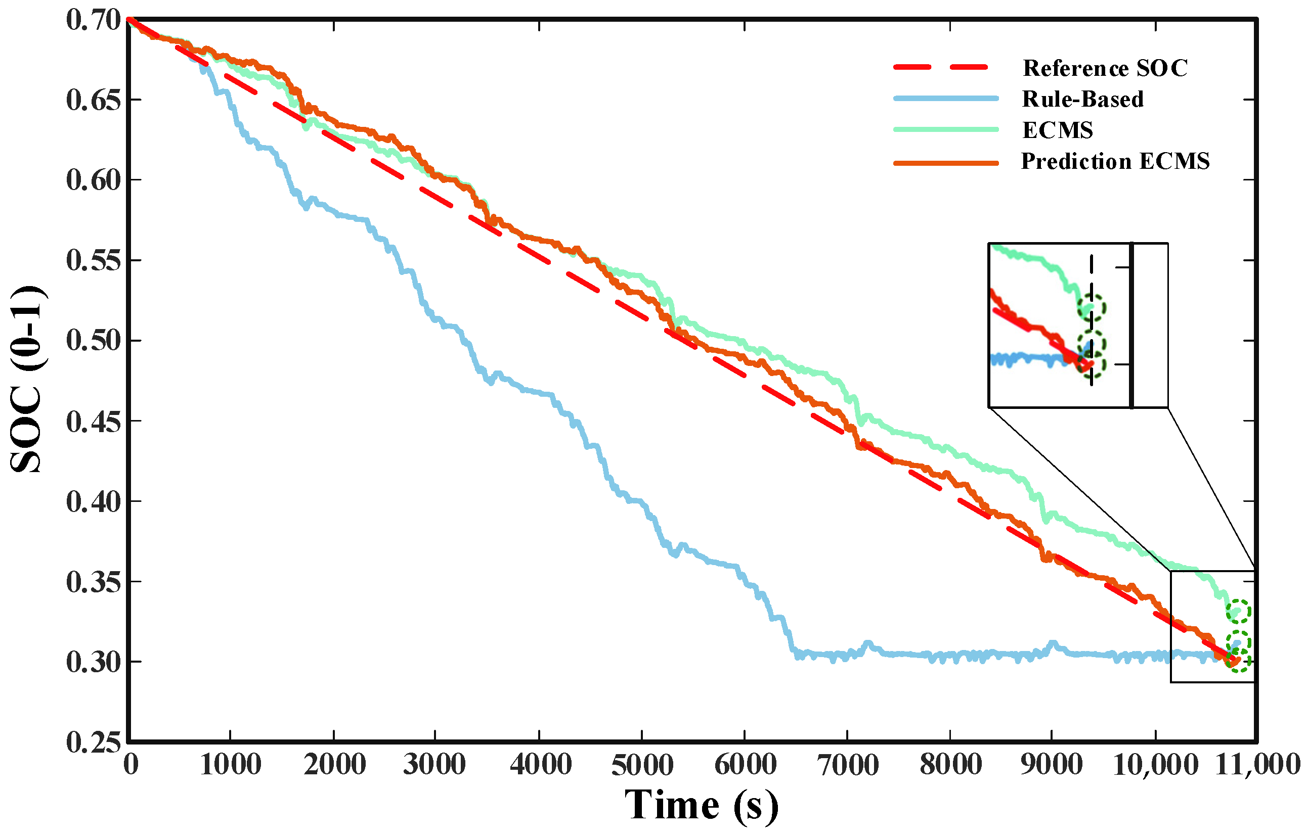
Figure 18 illustrates the battery SOC decline trajectories under different strategies, and Figure 19 shows the final values of fuel consumption and SOC under different strategies. It can be seen that the red dotted line represents the preplanned reference SOC trajectory; the SOC decline curves under both the rule−based and the ECMS−based strategies deviated from the planned SOC trajectory to a large extent during the trip. Among them, the SOC decline curve under the rule−based strategy first dropped sharply, and then maintained a dynamic stability near the desired SOC value in the middle and later stages of the stroke, and the power of the battery was difficult to be reasonably distributed. The downward trend of the SOC based on the ECMS strategy was more in line with the expected effect, but with the same initial equivalent factor as the adaptive strategy; the second half deviated from the set reference SOC trajectory, resulting in the final SOC only decreasing to 0.337, which is higher than the set expected SOC value of 0.30. The SOC drop trajectory proposed in this paper based on the driving cycle prediction strategy had small fluctuations, and the SOC was constrained to be near the planned reference SOC trajectory throughout the process; the final SOC was 0.303, which is very close to the expected value. This indicates that the introduced adaptive equivalent factor and PI controller could optimize the global battery power distribution.
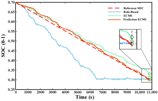
Figure 18.
SOC decline trajectories under different strategies.
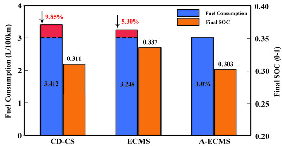
Figure 19.
Comparison of energy consumption under different strategies.
The energy simulation results of different strategies under 6*CLTC driving cycles are shown in Figure 19 and Table 4. It can be seen that, compared with the rule−based energy management strategy, the fuel consumption of the PHEV under the A−ECMS strategy after the introduction of driving cycle prediction was reduced by 9.85% to 3.076 L/100 km; even if it is comparable to the fuel consumption of the PHEV under the ECMS strategy, there was still a 5.30% decrease. This illustrates that the proposed adaptive energy management strategy based on driving cycle prediction could better exert the potential of PHEV and further reduce fuel consumption.
Table 4.
Fuel consumption under different strategies.
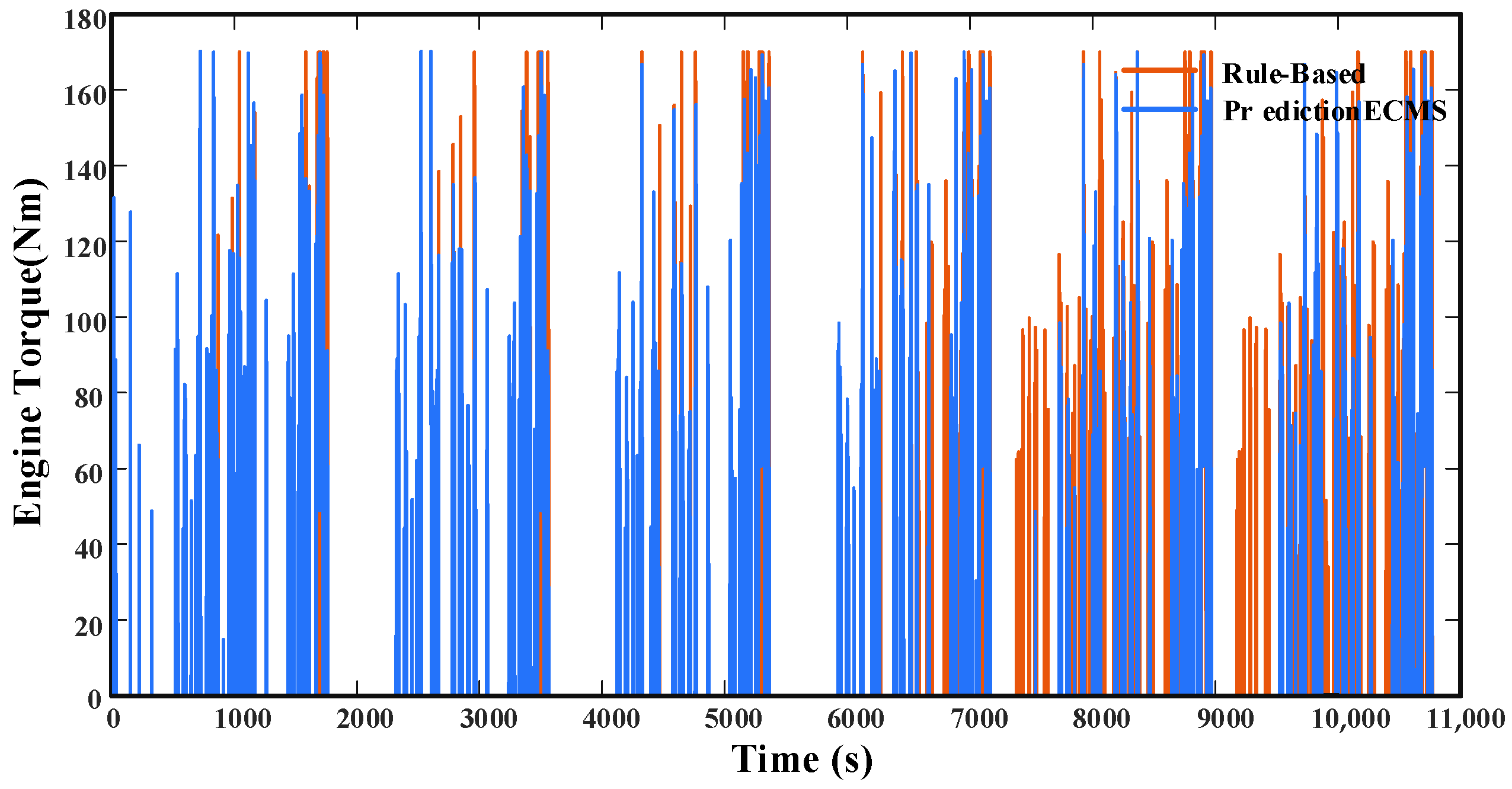
Figure 20 shows the comparison of engine torque based on the rule strategy and prediction strategy. It can be seen that, under the rule strategy, the engine would participate only when driving at high speed in CS mode. After entering the CD mode, the vehicle enters the feeding state, the subsequent driving tasks are mainly completed by the engine, and the motor only completes part of the driving and braking recovery functions. At this time, the engine spends more time in the low−efficiency working area, and the fuel consumption is relatively high. With the help of a strategy that includes predictive information, the engine can participate in driving at the right time throughout the journey, as well as cooperate with power components such as the motor to maintain a steady decline in the SOC of the power battery instead of only running when entering the CS stage.
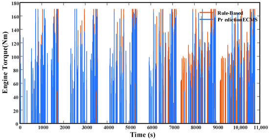
Figure 20.
Engine output torque under different strategies.
To sum up, the adaptive equivalent fuel consumption minimization strategy combined with vehicle speed information prediction could make the actual SOC follow the reference SOC during the trip, optimize the global power battery power distribution, and enable the engine to participate in driving while working in the high−efficiency area. Through the comparison of different strategies under the same working conditions, it was shown that the strategy reduced the fuel consumption and comprehensive energy consumption of the whole trip, and effectively improved the fuel economy of the whole vehicle.
7. Summary
In this study, a new vehicle speed prediction method was developed that combines the advantages of intelligent algorithms and artificial neural networks. The proposed model mainly optimized the initial weights and thresholds of the BP neural network through the particle swarm optimization algorithm, and the representative comprehensive driving cycles were selected as the training set of the neural network to improve the speed prediction accuracy during driving. Through a comparison with the exponential prediction model, the vehicle velocity information in the next 5 s was finally determined to be used for prediction to optimize the fuel economy of the PHEV. In addition, an adaptive energy management strategy based on prediction was proven, in which the torque of the engine and motor was allocated according to the principle of minimum instantaneous equivalent fuel consumption. Reference SOC and PI control were also introduced to optimize the global battery power allocation.
The simulation results under 6*CLTC−P driving cycles showed that the fuel consumption of the PHEV under the proposed adaptive energy management strategy was reduced by 9.85% compared with the classical rule−based strategy and by 5.30% compared with the ECMS strategy without prediction, thus further improving the fuel−saving efficiency of PHEVs.
Our research needs to be further advanced. Restricted to certain conditions, our current research mainly used the PSO−BP neural network to build a vehicle driving cycle prediction model, which is a prediction method established by learning historical data. However, many unexpected situations in the actual driving process often result in the vehicle not always following the ideal driving cycle. Lastly, we believe that the modification of the prediction model combined with the vehicle speed in the intelligent transportation system can further improve the fuel−saving potential of the PHEV.
Author Contributions
Data curation, Y.W.; methodology, K.L.; resources, R.L.; supervision, Y.W.; visualization, J.G.; writing—original draft, D.S.; writing—review & editing, S.L. All authors have read and agreed to the published version of the manuscript.
Funding
The research was funded by Hubei Provincial Department of Education: B2021210 and science and Technology Department of Hubei Province: 2020ZYYD001.
Institutional Review Board Statement
No applicable.
Informed Consent Statement
Not applicable.
Data Availability Statement
The data are available from the authors upon reasonable request.
Acknowledgments
This work was supported by the Central Government of Hubei Province to Guide Local Science and Technology Development (2020ZYYD001), the Guiding Project of Science and Technology Research Plan of Department of Education of Hubei Province (B2021210), and the Hubei Key Laboratory of Power System Design and Testing for Electrical Vehicles (ZDSY202206).
Conflicts of Interest
The authors declare no conflict of interest.
References
- Taherzadeh, E.; Radmanesh, H.; Mehrizi−Sani, A. A Comprehensive Study of the Parameters Impacting the Fuel Economy of Plug−In Hybrid Electric Vehicles. IEEE Trans. Intell. Veh. 2020, 5, 596–615. [Google Scholar] [CrossRef]
- Liu, K.; Guo, J.; Chu, L.; Yu, Y. Research on Adaptive Optimal Control Strategy of Parallel Plug−In Hybrid Electric Vehicle Based on Route Information. Int. J. Automot. Technol. 2021, 22, 1097–1108. [Google Scholar] [CrossRef]
- Tian, G.; Yuan, G.; Aleksandrov, A. Recycling of spent Lithium−ion Batteries: A comprehensive review for identification of main challenges and future research trends. Sustain. Energy Technol. Assess. 2022, 53, 102447. [Google Scholar] [CrossRef]
- Zhao, B.; Liu, R.; Shi, D. Optimal Control Strategy of Path Tracking and Braking Energy Recovery for New Energy Vehicles. Processes 2022, 10, 1292. [Google Scholar] [CrossRef]
- Han, W.; Chu, X.; Shi, S.; Zhao, L.; Zhao, Z. Practical Application−Oriented Energy Management for a Plug−In Hybrid Electric Bus Using a Dynamic SOC Design Zone Plan Method. Processes 2022, 10, 1080. [Google Scholar] [CrossRef]
- Liu, Y.; Li, J.; Gao, J. Prediction of vehicle driving conditions with incorporation of stochastic forecasting and machine learning and a case study in energy management of plug−in hybrid electric vehicles. Mech. Syst. Signal Process. 2021, 158, 107765. [Google Scholar] [CrossRef]
- Hao, J.; Yu, Z.; Zhao, Z. Optimization of key parameters of energy management strategy for hybrid electric vehicle using direct algorithm. Energies 2016, 9, 997. [Google Scholar] [CrossRef]
- Liu, L.; Zhang, B.; Liang, H. Global Optimal Control Strategy of PHEV Based on Dynamic Programming. In Proceedings of the 2019 6th International Conference on Information Science and Control Engineering (ICISCE), Shanghai, China, 20–22 December 2019; pp. 758–762. [Google Scholar]
- Chen, Z.; Liu, Y.; Zhang, Y.; Lei, Z.; Chen, Z.; Li, G. A neural network−based ECMS for optimized energy management of plug−in hybrid electric vehicles. Energy 2022, 243, 122727. [Google Scholar] [CrossRef]
- Liu, C.; Liu, Y. Energy Management Strategy for Plug−In Hybrid Electric Vehicles Based on Driving Condition Recognition: A Review. Electronics 2022, 11, 342. [Google Scholar] [CrossRef]
- Yang, C.; Zha, M.; Wang, W.; Liu, K.; Xiang, C. Efficient energy management strategy for hybrid electric vehicles/plug−in hybrid electric vehicles: Review and recent advances under intelligent transportation system. IET Intell. Transp. Syst. 2020, 14, 702–711. [Google Scholar] [CrossRef]
- Liu, J.; Chen, Y.; Zhan, J.; Shang, F. An on−line energy management strategy based on trip condition prediction for commuter plug−in hybrid electric vehicles. IEEE Trans. Veh. Technol. 2018, 67, 3767–3781. [Google Scholar] [CrossRef]
- Li, S.; Hu, M.; Gong, C.; Zhan, S.; Qin, D. Energy management strategy for hybrid electric vehicle based on driving condition identification using KGA−means. Energies 2018, 11, 1531. [Google Scholar] [CrossRef]
- Kazemi, H.; Fallah, Y.P.; Nix, A.; Wayne, S. Predictive AECMS by Utilization of Intelligent Transportation Systems for Hybrid Electric Vehicle Powertrain Control. IEEE Trans. Intell. Veh. 2017, 2, 75–84. [Google Scholar] [CrossRef]
- Ali, A.M.; Ghanbar, A.; Söffker, D. An online rolling optimal control strategy for commuter hybrid electric vehicles based on driving condition learning and prediction. IEEE Trans. Veh. Technol. 2015, 65, 4312–4327. [Google Scholar]
- Liu, T.; Tan, W.; Tang, X.; Zhang, J.; Xing, Y.; Cao, D. Driving conditions−driven energy management strategies for hybrid electric vehicles: A review. Renew. Sustain. Energy Rev. 2021, 151, 111521. [Google Scholar] [CrossRef]
- Shen, P.; Zhao, Z.; Zhan, X.; Li, J.; Guo, Q. Optimal energy management strategy for a plug−in hybrid electric commercial vehicle based on velocity prediction. Energy 2018, 155, 838–852. [Google Scholar] [CrossRef]
- Tian, G.; Fathollahi−Fard, A.M.; Ren, Y. Multi−objective scheduling of priority−based rescue vehicles to extinguish forest fires using a multi−objective discrete gravitational search algorithm. Inf. Sci. 2022, 608, 578–596. [Google Scholar] [CrossRef]
- Tian, G.; Chu, J.; Liu, Y. Expected energy analysis for industrial process planning problem with fuzzy time parameters. Comput. Chem. Eng. 2011, 35, 2905–2912. [Google Scholar] [CrossRef]
- Guo, H.; Du, S.; Zhao, F.; Cui, Q.; Ren, W. Intelligent Energy Management for Plug−in Hybrid Electric Bus with Limited State Space. Processes 2019, 7, 672. [Google Scholar] [CrossRef]
- Shi, D.; Liu, K.; Wang, Y.; Liu, R.; Li, S.; Sun, Y. Adaptive energy control strategy of PHEV based on the Pontryagin’s minimum principle algorithm. Adv. Mech. Eng. 2021, 13, 16878140211035598. [Google Scholar] [CrossRef]
- Zhang, L.; Liu, W.; Qi, B.N. Energy optimization of multi−mode coupling drive plug−in hybrid electric vehicles based on speed prediction. Energy 2020, 206, 118126. [Google Scholar] [CrossRef]
- Zhou, Y.; Ravey, A.; Péra, M.C. A survey on driving prediction techniques for predictive energy management of plug−in hybrid electric vehicles. J. Power Sources 2019, 412, 480–495. [Google Scholar] [CrossRef]
- Ke, H.; Liu, H.; Tian, G. An Uncertain Random Programming Model for Project Scheduling Problem. Int. J. Intell. Syst. 2015, 30, 66–79. [Google Scholar] [CrossRef]
- Tian, G.; Liu, Y.; Chu, J. Energy evaluation method and its optimization models for process planning with stochastic characteristics: A case study in disassembly decision−making. Comput. Ind. Eng. 2012, 63, 553–563. [Google Scholar] [CrossRef]
- Sun, C.; Hu, X.; Moura, S.J.; Sun, F. Velocity predictors for predictive energy management in hybrid electric vehicles. IEEE Trans. Control Syst. Technol. 2014, 23, 1197–1204. [Google Scholar]
- Zhang, Q.; Fu, X. A neural network fuzzy energy management strategy for hybrid electric vehicles based on driving cycle recognition. Appl. Sci. 2020, 10, 696. [Google Scholar] [CrossRef]
- Wang, N.; Zhu, X.; Zhang, J. License plate segmentation and recognition of Chinese vehicle based on BPNN. In Proceedings of the 2016 12th International Conference on Computational Intelligence and Security (CIS), Wuxi, China, 16–19 December 2016; pp. 403–406. [Google Scholar]
- Ren, T.; Liu, S.; Yan, G.; Mu, H. Temperature prediction of the molten salt collector tube using BP neural network. IET Renew. Power Gener. 2016, 100, 212–220. [Google Scholar] [CrossRef]
- Fathollahi−Fard, A.M.; Hajiaghaei−Keshteli, M.; Tavakkoli−Moghaddam, R. Red deer algorithm (RDA): A new nature−inspired meta−heuristic. Soft Comput. 2020, 24, 14637–14665. [Google Scholar] [CrossRef]
- Gharehchopogh, F.S.; Gholizadeh, H. A comprehensive survey: Whale Optimization Algorithm and its applications. Swarm Evol. Comput. 2019, 48, 1–24. [Google Scholar] [CrossRef]
- Ye, Y.; Yin, C.B.; Gong, Y.; Zhou, J.J. Position control of nonlinear hydraulic system using an improved PSO based PID controller. Mech. Syst. Signal Process. 2017, 83, 241–259. [Google Scholar] [CrossRef]
- Islam, M.R.; Ali, S.M.; Fathollahi−Fard, A.M.; Kabir, G. A novel particle swarm optimization−based grey model for the prediction of warehouse performance. J. Comput. Des. Eng. 2021, 8, 705–727. [Google Scholar] [CrossRef]
- Chen, H.Z.; Wang, X.D.; Cong, Y.P.; Yin, B. PSO−BP Neural Network for State−of−charge Estimation in a New Lithium Battery. In Software Engineering and Information Technology, Proceedings of the 2015 International Conference on Software Engineering and Information Technology (SEIT2015), Guilin, China, 26–28 June 2016; World Scientific: Singapore, 2016; pp. 310–316. [Google Scholar]
- Lin, X.; Wang, Z.; Wu, J. Energy management strategy based on velocity prediction using back propagation neural network for a plug-in fuel cell electric vehicle. Int. J. Energy Res. 2021, 45, 2629–2643. [Google Scholar] [CrossRef]
- Deng, Y.; Xiao, H.; Xu, J.; Wang, H. Prediction model of PSO−BP neural network on coliform amount in special food. Saudi J Biol Sci. 2019, 26, 1154–1160. [Google Scholar] [CrossRef] [PubMed]
- Li, J.; Liu, Y.; Qin, D.; Li, G.; Chen, Z. Research on equivalent factor boundary of equivalent consumption minimization strategy for PHEVs. IEEE Trans. Veh. Technol. 2020, 69, 6011–6024. [Google Scholar] [CrossRef]
- Deng, T.; Tang, P.; Luo, J.L. A novel real-time energy management strategy for plug-in hybrid electric vehicles based on equivalence factor dynamic optimization method. Int. J. Energy Res. 2021, 45, 626–641. [Google Scholar] [CrossRef]
- Zhou, M.; Zhong, C.; Li, J. Analysis of fuel consumption of China light duty vehicle test cycle for passenger car (CLTC−P). EDP Sci. 2021, 268, 01029. [Google Scholar] [CrossRef]


Publisher’s Note: MDPI stays neutral with regard to jurisdictional claims in published maps and institutional affiliations. |
© 2022 by the authors. Licensee MDPI, Basel, Switzerland. This article is an open access article distributed under the terms and conditions of the Creative Commons Attribution (CC BY) license (https://creativecommons.org/licenses/by/4.0/).