Prediction of Surface Subsidence of Deep Foundation Pit Based on Wavelet Analysis

Abstract

Predicting surface settlement in deep foundation pit engineering plays a central role in the safety of foundation pit construction. Recently, static or dynamic methods are usually applied to predict ground settlement in deep foundation pit projects. In this work, we propose a model combining wavelet noise reduction and radial basis neural network (XW-RBF) to reduce noise interference in monitoring data. The results show that the XW-RBF model predicts an average relative error of 0.77 and a root average square error of 0.13. The prediction performance is better than the original data prediction results with noise structure and has higher prediction accuracy. The noise data caused by the interference of construction and the surrounding environment in the original data can be removed via the wavelet noise reduction method, with the discreteness of the original data reducing by 30%. More importantly, our results show that the XW-RBF model can reflect the law of data change to predict the future data trend with high credibility. The findings of this study indicate that the XW-RBF model could optimize the deep foundation pit settlement prediction model for high accuracy during the prediction, which inspires the potential application in deep foundation pit engineering.

1. Introduction

The settlement prediction of foundation engineering plays a vital role in the development of the city. With the rapid development of cities and the rapid increase in traffic pressure, many cities vigorously develop subway projects to develop urban underground space. With the emergence of a large number of ultra-large-scale underground projects, the depth of excavation of deep foundation pits continues to increase, and engineering safety problems are becoming more serious. Therefore, there is an urgent need to predict surface subsidence accurately and its impact on the surrounding environment when formulating a support plan. Use this scheme to control the surface subsidence within a specific range and predict surface settlement to avoid disaster situations such as soil instability, uneven settlement of the surface, collapse, and other disasters [1,2,3].

Therefore, many scholars have devoted themselves to the settlement prediction of deep foundation pits in different foundation projects [4,5]. In the early 20th century, Karl Terzaghi et al. [6] established a classical foundation settlement analysis method, named the “Terzaghi One-Dimensional Consolidation Theory”, suitable for the slight deformation of saturated soil. The theory is the beginning of modern soil mechanics, but the theory is not suitable for calculating soft soil foundations. Since then, other researchers have contributed to the improvement and refinement of the method. The foundation deformation and settlement prediction methods can be divided into two categories from the basic principle: one class is based on a formula or theory. The static prediction method uses the measured settlement data for fitting, and another class of dynamic forecasting methods, such as GM (Gray Theory Method) [7]. On the research road of static prediction methods, Ismail and Jeng [8] proposed a new neural network model in 2011. The Standard Penetration Test data [9] along the excavation depth direction of the pile foundation is used as input samples, then calculates the load-settlement curve and predicts subsequent settlement. Nejad and Jaksa [10] established Artificial Neural Network [11] and Cone Penetration Test [12] data to model load settlement. At the same time, the overall load–settlement relationship is obtained. Additionally, for the dynamic prediction method, Lv et al. [13] proposed a new model for calculating settlement around foundation pits based on grey theory and BP neural network. However, the model error is still significant, and time is still the only input factor to consider. Su et al. [14] proposed a settlement monitoring method based on the Kalman filter [15]. The settlement was studied by forward modeling. The result shows it can predict the next stage’s deformation by analyzing the previous stage’s data. However, the prediction accuracy of the above methods is not high enough. The reason for the low accuracy may be that the project contains large noise data due to the process or environmental impact monitoring data. This also leads to large fluctuations in monitoring data, which affects the forecast results.

The combination of wavelet noise reduction and neural networks can more accurately predict the surface settlement of foundation engineering. In recent years, wavelet theory has developed rapidly. By virtue of its good time-frequency characteristics in the field of noise reduction, wavelet theory has attracted the attention of many scholars. They applied wavelets for noise reduction and got excellent results. For example, applying wavelet noise reduction to images can remove unnecessary noise and preserve the more important details and other information in the image. It makes the resulting image appear sharp and clean [16]. Dmitry et al. [17] have combined wavelet and neural networks to denoise images. However, this article does not use the prediction function of neural networks, and there are many types of neural networks and wavelet, and different types of neural networks and wavelet have different effects on the results. The main purpose of this paper is to prove that the combination of wavelet and neural networks can effectively predict land subsidence in engineering. The combined effects of different types of wavelets and neural networks are expected to be discussed further in future articles. Therefore, according to the advantages of wavelet noise reduction, we tried to use a wavelet to process the monitoring data of foundation settlement in the project. The purpose is to remove the noise data, and then the denoised numbers are imported into the neural network for learning prediction and observing the prediction effect.

In this work, we use an engineering example to illustrate the accuracy of a wavelet neural network in predicting the surface settlement of deep foundation pits. This study takes the deep foundation pit project of Nantong East Station of Nantong Metro Line 2 in China as the research object using the wavelet neural network method, the settlement of deep foundation pits is simulated and estimated. Then, the neural network method is introduced to predict the settlement of deep foundation pits and compare the prediction results of the two methods with the field monitoring data. It is concluded that the prediction data will be more accurate after wavelet noise reduction. Finally, the law of surrounding soil settlement during the construction of a deep foundation pit is summarized. To provide a reference for the construction and optimization design of the subway deep foundation pit project in the Nantong area.

2. Wavelet Noise Reduction and Network Prediction

Wavelets are widely used in signal analysis. The previous study reported that the wavelets could be used for boundary processing and filtering, time-frequency analysis [18], signal-to-noise separation and extraction of weak signals [19], fractal index calculation, signal identification, and diagnosis [20]. Wavelet analysis has the advantage of characterizing local features in both the time and frequency domains of the signal [21]. Therefore, wavelet analysis has become one of the main tools in signal processing. It is a milestone in the history of the development of reconciliation analysis. Artificial Neural Networks (ANNs) are called Neural Networks (NNs). ANNs is a mathematical model that imitates the behavioral characteristics of animal neural networks [22]. The model enables distributed parallel information processing algorithms. The model depends on the complexity of its own system and achieves the purpose of processing information by adjusting the interconnection relationship between a large number of internal nodes. The work first uses the wavelet noise reduction method to process the original processing to obtain smoother data and improve the model’s prediction accuracy. Then, the processed raw data is divided into the training set and test set, and a neural network is constructed using the data of the training set. Finally, the test set data is imported into the neural network to verify the prediction accuracy.

2.1. Wavelet Decomposition Noise Reduction

The wavelet decomposition noise reduction method is an algorithm based on the wavelet transform. The basic idea is to distinguish the low-frequency signal (the smooth part of the original signal) and the high-frequency signal (the original signal detail part) according to the characteristics of different intensity distributions of the wavelet decomposition coefficients of the noise and the signal in different frequency bands. Then, the information-rich low-frequency signal is finally preserved. The wavelet transforms [23] is a localized analysis of time (space) and frequency. It gradually performs multi-scale refinement on the signal (function) through scaling and translation operations. Finally, time subdivisions at high frequency and frequency subdivisions at low frequency are achieved, which can automatically adapt to the requirements of time-frequency signal analysis. This allows focusing on any details of the signal.

Wavelet transformation is the basis of wavelet decomposition and noise reduction. It is a method used to decompose a continuous time function [24] into several wavelets. Then, it can construct a time-frequency signal with good time-domain and frequency-domain localization. Mathematically, a function x(t) that has continuous-time properties and is integrable can be represented by the following integral:

$${\mathrm{X}}_{\mathrm{W}}\left(\mathrm{a},\mathrm{b}\right)=\frac{1}{\sqrt{\left|\mathrm{b}\right|}}{{\displaystyle \int }}_{-\infty }^{\infty }\mathrm{x}\left(\mathrm{t}\right)\mathsf{\psi }\left(\frac{\mathrm{t}-\mathrm{a}}{\mathrm{b}}\right)\mathrm{dt}$$

$\mathsf{\psi }\left(\mathrm{t}\right)$ is the mother wavelet function (Mother Wavelet) where a is called the scale factor and represents the translation position, and b is called the translation factor and represents the scaling, it is a function with continuous properties in both time domain and frequency domain.

After wavelet transformation, the obtained wavelet signals are filtered according to a set of decomposition filters H (low-pass filter) and G (high-pass filter), in the Mallat algorithm [25]. The output result is down-sampled (referring to taking one every other) to achieve wavelet decomposition. The decomposition results in producing two parts of halved length: the smoothed part of the original signal produced by the low pass filter and the detailed part of the original signal produced by the high pass filter.

$$\mathrm{x}\left(\mathrm{t}\right)={\mathrm{c}}_{\mathrm{j},\mathrm{k}}{\displaystyle \sum }_{\mathrm{k}}{\mathsf{\phi }}_{\mathrm{j},\mathrm{k}}+{\mathrm{d}}_{\mathrm{j},\mathrm{k}}{\displaystyle \sum }_{\mathrm{k}}{\mathsf{\psi }}_{\mathrm{j},\mathrm{k}}$$

In the expression, the first term is the low-frequency part of the signal $\mathrm{x}\left(\mathrm{t}\right)$ whose frequency does not exceed $2^{-\mathrm{j}/2}$, and the second term is the high-frequency the signal $\mathrm{x}\left(\mathrm{t}\right)$ whose frequency is between $2^{-\mathrm{j}/2}$ and $2^{\left(-\mathrm{j}+1\right)/2}$, where ${\mathrm{c}}_{\mathrm{j},\mathrm{k}}$ is the low-frequency coefficient of the wavelet transform on the largest scale and ${\mathrm{d}}_{\mathrm{j},\mathrm{k}}$ is the high-frequency coefficient decomposed by each layer. So, if the decomposed high-frequency part of the signal (noise) is set to 0, the low-frequency part of the signal after noise reduction (smooth signal) can be obtained. The high-frequency signal is generated due to the influence of the construction process or the surrounding environment during the construction process. The high-frequency signal appears to produce high-frequency vibrations. Therefore, the high-frequency signal represents the noise part of the surface subsidence monitoring value. The low-frequency signal is caused by the continuous excavation of the soil during the construction process. Represents the real surface subsidence value.

Wavelet transform is divided into two categories: discrete wavelet transform (DWT) and continuous wavelet transform (CWT). The main difference between discrete and continuous wavelet transforms is that the continuous transform operates on all possible scaling and shifts, while the discrete transform takes a specific subset of all scaling and shifts. Therefore, a continuous wavelet is suitable for the direct analysis of continuous data. However, when the data needs to be processed by a computer, the input is often only some discrete data, then you need to use discrete wavelet transform for processing. In this paper, wavelet transform is used to denoise monitoring data, so discrete wavelet transform is needed. When using wavelet decomposition to denoise the signal, commonly used wavelet functions are Haar wavelet, Mexican Hat wavelet, Morlet wavelet, Meyer wavelet, and Daubechies wavelet. The Haar wavelet is discontinuous in the time domain, so its performance as a basic wavelet is not particularly good. Mexican Hat wavelet is good localization in the time domain and frequency, but there is no scaling function, so this wavelet function is not orthogonal. Morlet wavelets are single-frequency sinusoidal functions under a Gaussian envelope. Morlet wavelet has no scaling function and is a non-orthogonal decomposition. Meyer wavelet’s wavelet and scaling function are defined in the frequency domain. Among them, Daubechies wavelet is also known as dbN wavelet, and N is the order of the wavelet [18,26,27,28,29]. A large number of data shows that the dbN wavelet has good regularity [30]. The smooth error introduced by the wavelet as a sparse basis is not easy to detect [31], which makes the signal smoother after decomposing and denoising. Each wavelet has different properties, so the predictive power of each wavelet is different. However, the Daubechies wavelet has a better frequency band division effect, and has a better effect and neural networks combine different effects. In future research, we will discuss the impact of different wavelet and neural network combinations on the prehe data, and the denoising effect of other wavelets will be carried out in future research. In conclusion, the study uses the db12 wavelet to process the measured settlement data and obtains the actual settlement data signal (low-frequency signal) of the foundation pit.

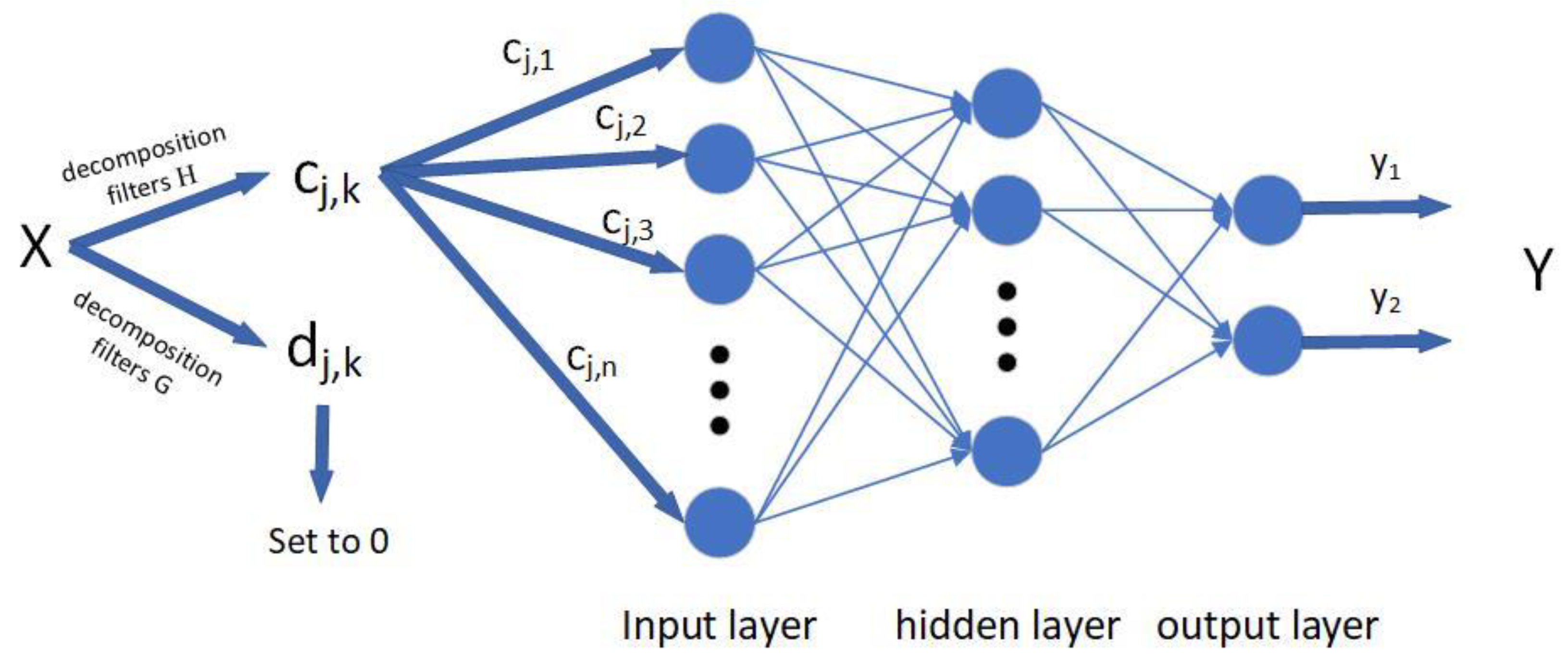
2.2. Wavelet Network Prediction Model

The evolution of soil stress and deformation is a typical nonlinear problem [32], and its evolution process is highly nonlinear and complex. Most of the previous research on the prediction of foundation pit precipitation and settlement uses the methods of establishing empirical formulas and numerical analysis. However, these methods are challenging to predict foundation pit settlement accurately. In recent years, intelligent methods have been developed to describe the highly nonlinear relationship of geotechnical mechanics with black-box or grey-box structures [33], avoiding the explicit expression of complex nonlinear structures. The neural is through the input of multiple nonlinear models and the weighted interconnection between different models (the weighting process is done in the hidden layer). Finally, an output model is obtained, in which the hidden layer represents a nonlinear function. Figure 1 is the principle diagram of a wavelet neural network. The study uses the RBF network [34], compared with the traditional BP neural network. This model has higher accuracy, can handle hard-to-resolve regularities in the system and has a faster learning speed.

The RBF neural network model is a forward neural network structure proposed by Moody and Darken [35] in 1988. The principle is to use RBF as the “base” of the remote unit to form the hidden layer space. This makes it possible to map the input vector directly into the latent space without connecting via weights. When the center point of the RBF is determined, the mapping relationship is also determined. Moreover, the mapping from the hidden layer space to the output space is linear, where the network’s output is a linear weighted sum of the outputs of the hidden units. The weights here are tunable network parameters. The function of the hidden layer is to map the vector from the low-dimensional p to the high-dimensional h so that the low-dimensional linear inseparability can become linearly separable from the high-dimensional. This is the idea of using the kernel function [36].

In the study, the surface subsidence monitoring data is firstly decomposed by wavelet multi-scale [37] to obtain the denoised subsidence data, then construct the RBF neural network model (W-RBF for short) based on the settlement date. Finally, the actual settlement data is compared with the predicted data to judge whether the construction accuracy is satisfied. The realization of settlement prediction mainly consists of the following steps:

(1)

Using the db wavelet to decompose the settlement monitoring data and obtaining the training sample set of the prediction model by eliminating high-frequency signals.

(2)

Using the training sample set, build and train the W-RBF prediction model.

(3)

Using the test data set to verify the accuracy of the W-RBF model.

(4)

Predict the surface subsidence value.

The W-RBF model structure consists of two modules, and its prediction flow chart is shown in Figure 2.

3. Project Overview

3.1. Engineering Background

Nantong East Station of Nantong Metro Line 2 is a two-story underground station. The station is located at the intersection of Qingnian East Road and the Donghuan Expressway. The station is set underground along Qingnian East Road from east to west. The station outsourcing size is 202.6 m in total length, the width of the standard section is 20.7 m, and the width of the end section is 25.2 m. According to the geotechnical investigation report and regional experience, the physical mechanics of soil parameters related to foundation pit support are shown in

Table 1. Mechanical parameters of rock mass of deep foundation pit.

Soil Layer Name	Layer Thickness/m	Unit Weight of Soil (kN/m2)	Modulus of Compressibility/MPa	Poisson’s Ratio	Cohesion/kPa	The Angle of Internal Friction/(°)
miscellaneous fill layer	2.0~3.8	18			10	18
Clayey and powdery soil layer	2.2~4.2	18.4	6.7	0.480	14.2	25.4
powdery sand with sandy and powdery soil	5.1~8.8	19.4	11.5	0.484	5.6	33.2
powdery sand layer	5.1~7.8	19.0	10.9	0.486	7.8	30.7
powdery and meticulous sand layer	1.7~5.1	19.6	13.0	0.485	4.8	33.4
Powdery silt	2.9~6.2	17.4	3.4	0.485	22.8	15.6
Powdery silt with sandy and powdery soil	1.5~5.2	17.8	5.4	0.492	14.5	25.5
sandy and powdery soil with powdery sand	9.6~13.1	17.6	6.4	0.491	12.4	27.1
Clayey and powdery soil layer with powdery sand	11.2~17.1	17.7	9.0	0.484	10.2	28.7

.

3.2. Hydrogeological Conditions

According to the geological survey report, during the survey period, the stable diving water level in the site is 1.50–3.10 m above sea level. According to regional data, in the past 3 to 5 years, the highest diving level is about 3.50 m in the national elevation reference, the lowest diving level is about 1.50 m, and the annual variation range is generally 1–2 m. I1 Confined water generally occurs in silt mixed with silt at a depth of less than 30 m, and I2 Confined water generally occurs in silt mixed with silt at a depth of less than 50 m. According to the regional hydrogeological data of I1 confined water and I2 confined water, the water head is buried 2–5 m below the natural ground.

3.3. Construction Technology and Monitoring Layout

The main building envelope of the station adopts an 800-thick underground diaphragm wall with internal support. The body structure adopts a cast-in-place reinforced concrete box structure [38,39], the maintenance structure and the main structure form a composite wall structure, and the structure set an all-inclusive waterproofing. The foundation pit structure adopts H-shaped steel joints. The design service life shall be considered as not less than one year but not more than two years. The first support adopts eco-friendly concrete support [40], the second and third steel supports use ⏀800 and t = 20, and the rest are supported by ⏀600, t = 16 steel. The workload of leak detection is the main structure of the station. The total length is 82 m. The detection area is divided into two detection areas, A and B. There are 77 detection sensors in total. As shown in Figure 3, the monitoring work scope includes the following:

(1)

All excavation surfaces and supporting systems of the station foundation pit;

(2)

The monitoring range of surface settlement is taken as the 3H range on both sides of the edge of the foundation pit;

(3)

The monitoring range of the flexible pipeline is taken as the 2H range on both sides of the edge of the foundation pit; the monitoring range of rigid or pressure underground pipelines such as water supply, rainwater, and sewage shall be taken as the 3H range on both sides of the edge of the foundation pit;

(4)

Considering the influence of the precipitation of the confined water, the settlement range of the building shall be expanded to the 5H range on both sides of the edge of the foundation pit; when the confined water is not lowered, the monitoring range is taken as the 3H range on both sides of the edge of the foundation pit; after the confined water dewatering well is opened, the monitoring range of building settlement should be increased according to the precipitation situation.

4. Engineering Applications

4.1. Selection of Wavelet Parameters

The graphs of settlement monitoring data for measurement points 2−2 and 2−4 were found to contain a large amount of noise in the raw data. The data shows from Figure 4 that the settlement curves of measuring points 2−2 and 2−4 have strong fluctuations. For example, from the 60th to the 125th day, the settlement curve fluctuated violently in the range of 12.5–15 mm. It is guessed that it is caused by the noise generated by the construction process and construction environmental factors, which is not conducive to the subsequent settlement prediction. Therefore, the two-point settlement data are decomposed and de-noised by wavelet transform to remove the noise in the signal. In the project introduced in the study, due to the influence of the surrounding environment and construction technology during the construction of the foundation pit [41], the monitoring data of foundation pit surface settlement must contain noise data, which makes the detection data fluctuate violently locally, making the prediction more difficult. Here, it is assumed that the monitoring data of these two points are:

x(t) = S(t) + e(t)

where S(t) is the data signal reflecting the changing trend of the actual subsidence of the surface, it is characterized by a low-frequency signal in the frequency domain and a relatively regular smooth signal as a whole; e(t) is a noise signal, which generally appears as a high-frequency signal in the frequency domain. Therefore, a set of high-frequency signals e(t) can be obtained by wavelet decomposition of x(t) and set to 0, which can separate the real signal from the noise and achieve the purpose of noise reduction.

The graphs of the noise reduction treatment are compared with the curves of the monitoring data, and the advantages of the noise reduction treatment are analyzed. In the study, the 12-order db wavelet with good noise reduction effect is used to analyze the settlement data signal, comparing the noise reduction effects of wavelet noise reduction scales of 3, 4, and 5 and selecting the most appropriate scale. The change curve of surface subsidence after noise reduction is shown in Figure 5. Analysis of Figure 5 clearly shows that the low-frequency data curve obtained from the 60th to the 150th day after the original monitoring data is processed by db12 noise reduction is smoother and more regular. Analysis of Figure 5 clearly shows that the low-frequency data curve obtained from the 60th to the 150th day after the original monitoring data is processed by db12 noise reduction is smoother and more regular. The standard deviation is introduced here to reflect the volatility of the curve. According to previous experiments, surface monitoring data in deep foundation pit engineering is often affected by noise. The cause of the noise is the vibration generated during construction and the influence of the surrounding environment. These factors produce high-frequency noise data. Therefore, noise results in high fluctuation of monitoring data. Discreteness is used here to reflect the denoising level. The standard deviation is introduced here to reflect the discreteness of the curve. The standard deviation, also known as the standard deviation, is the arithmetic square root of the arithmetic mean squared from the mean (variance) [42]. Standard deviation can reflect the degree of dispersion of a data set. By calculation, the standard deviations of the settlement date of the measured points 2−2 after the third-order wavelet noise reduction and the unprocessed curve between 60 days and 150 days are 0.39 and 0.56, respectively. After wavelet noise reduction processing, the discreteness is reduced by 30%, so the curve change trend is more gentle and more regular after noise reduction processing. However, the changing trends of wavelet denoising curves of different orders are relatively close. To more clearly reflect the effect of wavelet denoising of different orders and try to reduce the error caused by wavelet denoising, Figure 6 represents the data error curve of different scales of wavelet denoising.

Figure 6 shows the error curves after wavelet noise reduction at different scales, and it is found that the wavelet noise reduction effect with a scale of three is the best. According to the analysis of Figure 6, which can be obtained that the error range of the data after wavelet processing of the three scales is within ±3.5 mm, and the error is small. Among them, the db12 wavelet with a scale of three has the best noise reduction effect, and the error range is less than ±2.0 mm. Moreover, within the range from the 10th day to the 25th day of measurement points 2−2 and the 30th to the 50th day of measurement points 2−4, the wavelet noise reduction curve with scale three is more apparent and closer to the fluctuation trend of the original data. In summary, the wavelet noise reduction data curve with a scale of three can better represent the detailed characteristics of the original data and the actual settlement trend. Therefore, it can be concluded that after the original settlement monitoring data is denoised by the db12 wavelet with a scale of three, the detailed features in the monitoring settlement data can be retained, and the noise in them can be removed, making the settlement data curve smoother and more regular.

4.2. Prediction and Analysis of Surface Subsidence

In this study, the combination of wavelet noise reduction and neural network is applied to predict the settlement of measuring points 2−3 and points 2−5 in foundation pit engineering First, use the third-order db12 wavelet to denoise the original monitoring data of measuring points 2−3 and points 2−5, and then use the RBF neural network model to predict the settlement data of measuring points 2−3 and points 2−5. The number of data in the training set is 200, which is used to train and construct the RBF neural network, and the remaining data is included in the test set to verify the accuracy of the prediction of the constructed RBF neural network. In the RBF model, the parameters were set as: radial basis diffusion velocity 77, mean square error target 0.0, the maximum number of neurons 300, and network parameter 50 added each time. Additionally, import every 20 data in the training set as a group into the RBF neural network to learn the relationship between the 20 data and the latter data to obtain the law, after the training, the accuracy of the trained RBF neural network is checked with the test set data.

We found that the predicted data after 100 in the prediction results are more accurate by analyzing Figure 7 and Figure 8. To verify the influence of wavelet decomposition and noise reduction on settlement prediction, in the study, the RBF neural network is also used to directly predict the monitoring data without noise reduction processing and the detection data after noise reduction processing to predict and compare. Figure 7 presents the comparison curves of the predicted and measured values in two different situations. To find out which method has a better prediction effect in different situations, Figure 8 is the curve comparison diagram of the error generated by the prediction value of two different methods. The curves can be found that the prediction results of the first 100 data of the training set after wavelet noise reduction have large errors, but the subsequent predictions are more accurate. By analyzing Figure 6, the error curve is found that the error of the first 100 data after wavelet processing is larger than the original data, which leads to the larger error of the subsequent prediction results after wavelet processing. It is speculated that these results are caused by the boundary effects produced by the wavelet processing.

A new prediction model is put forward according to the data change pattern of the error comparison chart Figure 8. According to the images, it can be found that the error of the simulated data of measuring points 2−5 suddenly increased around the 25th day. According to the analysis of the original data, the monitoring data suddenly increased on the 33rd day, and the monitoring settlement value returned to the original level on the 34th day. It is guessed that this is due to the error caused by the construction process or the surrounding environment, and the actual settlement value has not changed so much. Therefore, it can be concluded that the data after wavelet denoising is more in line with the actual situation through simulation prediction. Additionally, according to the above analysis, the first 100 data simulated by the RBF neural network without wavelet noise reduction is more accurate. However, the error of the data predicted by the W-RBF model was controlled within ±0.5 mm. In contrast, the error value of the predicted data of the RBF model fluctuated within ±1.0 mm, so the data after noise reduction was more accurate. However, the first hundred data errors predicted by the W-RBF model are larger than those predicted by the RBF model. Therefore, a new XW-RBF model is proposed to further increase the prediction accuracy. The difference between the XW-RBF model and the W-RBF model is that its first one hundred data are not processed by wavelet. Figure 9 is the comparison curve between the predicted and measured results of the (XW-RBF) model and the RBF model without noise reduction. The prediction results of the XW-RBF model obtained by analysis are more in line with the moving trend of the original data. To get the prediction effect of the new model more clearly, Figure 10 is a curve comparison chart of the error generated by the prediction values of the two models.

Figure 10 shows the new wavelet model has higher prediction accuracy than the model without wavelet processing. Analysis of Figure 10 shows that the prediction results of the first 100 data of the new model are much more accurate than the W-RBF model. Additionally, then, the data error is smaller than most of the results predicted by the model without wavelet processing. To more clearly reflect the prediction accuracy after wavelet processing, using average relative error rate (ARER) and the root means square error (RMSE) of measuring points 2−3 is used to analyze and evaluate the performance of the prediction and the accuracy of the model (the smaller the root mean square error and the better the prediction effect), the formula:

$$\mathrm{ARER}=\frac{1}{\mathrm{n}}{\displaystyle \sum }_{\mathrm{t}=1}^{\mathrm{n}}\left|\frac{\mathrm{S}\left(\mathrm{t}\right)-\mathrm{f}\left(\mathrm{t}\right)}{\mathrm{f}\left(\mathrm{t}\right)}\right|\times 100\%$$

$$\mathrm{RMSE}=\sqrt{\frac{{{\displaystyle \sum }}_{\mathrm{t}=1}^{\mathrm{n}}{\left[\frac{\mathrm{S}\left(\mathrm{t}\right)-\mathrm{f}\left(\mathrm{t}\right)}{\mathrm{f}\left(\mathrm{t}\right)}\right]}^2}{\mathrm{n}}}$$

In the formula, $\mathrm{S}\left(\mathrm{t}\right)$ is the predicted value of settlement, $\mathrm{f}\left(\mathrm{t}\right)$ is the measured value of settlement, n is the number of predicted samples, and draw

Table 2. Comparison between measured and predicted settlements of measuring points 2−3.

Model	Model Precision/mm	Average Error Rate/%	Maximum Error/mm
XW-RBF model	0.13	0.77	0.47
RBF model	0.17	1.02	0.85

.

For the predictive data of Table 2, the prediction results of the XW-RBF model are better than the RBF model in all aspects. According to Table 2, under the same conditions, the accuracy of the XW-RBF model is more accurate than that of the RBF model (without wavelet processing), and the accuracy is 0.13 mm; the average error rate is 0.77%, which is 25% lower than that of the RBF model; and the maximum error is 0.47 mm, which is nearly doubled compared to the RBF model. In summary, the XW-RBF model is superior to the prediction results of the RBF model in all aspects. It can be concluded that the predicted value of the XW-RBF model is in good agreement with the measured value. Compared with other models, the XW-RBF model has a minor error and higher prediction accuracy, which can meet the needs of surface settlement prediction of deep foundation pit engineering.

According to the settlement trend graph after wavelet noise reduction, the time-frequency analysis of the measuring points is carried out. The settlement of these four measuring points develops over time and the surface settlement increases with the excavation depth of the foundation pit. During the excavation, the growth rate of the settlement was fast, and with the completion of the construction of the floor and internal structure, the settlement gradually stabilized. Affected by the prestress of the steel support, a large reverse thrust is provided when the support is erected, which will inhibit the subsidence of the ground or even lift the ground, resulting in a slowdown or even a decrease in the settlement of the surface measuring points. However, this effect decreases with the continued excavation of the earthwork, which is the reason for the fluctuation-like growth of the surface subsidence duration curve. On the other hand, the surface settlement of measuring points 2−5 is obviously smaller than that of other measuring points, which is guessed because measuring points 2−5 are farther away from the main construction point.

5. Conclusions and Outlooks

In this study, 3Ndb wavelet noise reduction and RBF neural network were selected to predict the settlement of the deep foundation pit surface and explore a more accurate prediction method for the deep foundation pit surface settlement. The purpose is to find out the law of surface subsidence, to guide the formulation of the support scheme, and to ensure the construction safety of the underground engineering project. According to the different time-frequency characteristics of actual signal and noise in the measured surface subsidence data, the study uses wavelets to perform multi-scale decomposition. It realizes the noise separation in the surface subsidence data and obtains the real subsidence value. On the other hand, the study proposes the idea of wavelet noise reduction to more clearly reflect the characteristic quantities of surface monitoring subsidence data. Using the radial basis neural network model to predict and analyze the surface subsidence can improve the prediction accuracy of the model. The results show that compared with the RBF neural network without wavelet processing, the prediction error rate is reduced by 25%, and the accuracy is improved by 24%. Finally, the engineering application results show that the wavelet network XW-RBF model can predict surface subsidence with high prediction accuracy. Therefore, we can conclude the XW-RBF model can reflect the law of data change to predict the future data trend with high credibility.

Overall, the study concluded that wavelet decomposition to denoise monitoring data is an effective method to obtain actual settlement values, which can improve the accuracy of surface settlement prediction for deep foundation pits. However, the newly proposed wavelet neural model does not require wavelet denoising for the first one hundred data, which increases the complexity of the prediction process. Moreover, the basis of the model construction in the study is based on some monitoring data that have been measured before. However, how much monitoring data is needed to establish the model accurately and the influence of the changes of some parameters in the wavelet and neural network used on the prediction results need to be further discussed. Therefore, based on the work, it is possible to further study how much monitored data is needed to train the XW-RBF neural network and the optimal parameters of the wavelet and neural network used in practical engineering. In addition, there are many kinds of wavelets and neural networks proposed now. However, different wavelets and neural networks combine different effects. In future research, we will discuss the impact of different wavelet and neural network combinations on the prediction performance based on the current existing work, so as to obtain a model with better prediction performance.

Finally, the engineering application results show that the wavelet network XW-RBF model can predict surface subsidence with high prediction accuracy. This model can be used to control the surface settlement within a certain range, predict the surface settlement, and avoid soil instability, surface uneven settlement, collapse, and other disasters. The obtained performance is higher than the prediction result of the original data, which can meet the construction requirements, and has certain practicability in the information construction of deep foundation pit engineering.

References

1. Wang, P.; Ma, S.; Yue, Z.; Lu, C.; Tian, S.; Li, A. A theoretical study on the spatial effect of water-rich foundation pit instability failure. AIP Adv. 2021, 11, 015049. [Google Scholar] [CrossRef]
2. Yang, W.; Hu, Y.; Hu, C.; Yang, M. An agent-based simulation of deep foundation pit emergency evacuation modeling in the presence of collapse disaster. Symmetry 2018, 10, 581. [Google Scholar] [CrossRef] [Green Version]
3. Liu, L.; Wu, R.; Congress, S.S.C.; Du, Q.; Cai, G.; Li, Z. Design optimization of the soil nail wall-retaining pile-anchor cable supporting system in a large-scale deep foundation pit. Acta Geotech. 2021, 16, 2251–2274. [Google Scholar] [CrossRef]
4. Zhou, Y.; Li, S.; Zhou, C.; Luo, H. Intelligent approach based on random forest for safety risk prediction of deep foundation pit in subway stations. J. Comput. Civ. Eng. 2019, 33, 05018004. [Google Scholar] [CrossRef]
5. Liu, Q.; Yang, C.Y.; Lin, L. Deformation Prediction of a Deep Foundation Pit Based on the Combination Model of Wavelet Transform and Gray BP Neural Network. Math. Probl. Eng. 2021, 2021, 2161254. [Google Scholar] [CrossRef]
6. Terzaghi, K.; Peck, R.B.; Mesri, G. Soil Mechanics in Engineering Practice; John Wiley & Sons: Hoboken, NJ, USA, 1996. [Google Scholar]
7. Wang, Y.; Yang, G. Prediction of Composite Foundation Settlement Based on Multi-Variable Gray Model. In Proceedings of the Applied Mechanics and Materials; Trans Tech Publ.: Stafa-Zurich, Switzerland, 2014. [Google Scholar]
8. Ismail, A.; Jeng, D.-S. Modelling load–settlement behaviour of piles using high-order neural network (HON-PILE model). Eng. Appl. Artif. Intell. 2011, 24, 813–821. [Google Scholar] [CrossRef]
9. Nixon, I.K. Standard penetration test State-of-the-art report. In Proceedings of the Penetration Testing; Routledge: London, UK, 2021. [Google Scholar]
10. Nejad, F.P.; Jaksa, M.B. Load-settlement behavior modeling of single piles using artificial neural networks and CPT data. Comput. Geotech. 2017, 89, 9–21. [Google Scholar] [CrossRef]
11. Tealab, A. Time series forecasting using artificial neural networks methodologies: A systematic review. Future Comput. Inform. J. 2018, 3, 334–340. [Google Scholar] [CrossRef]
12. Fang, K.; Zhao, T.; Zhang, Y.; Qiu, Y.; Zhou, J. Rock cone penetration test under lateral confining pressure. Int. J. Rock Mech. Min. Sci. 2019, 119, 149–155. [Google Scholar] [CrossRef]
13. Lv, Y.; Liu, T.; Ma, J.; Wei, S.; Gao, C. Study on settlement prediction model of deep foundation pit in sand and pebble strata based on grey theory and BP neural network. Arab. J. Geosci. 2020, 13, 1–13. [Google Scholar] [CrossRef]
14. Su, J.; Xia, Y.; Xu, Y.; Zhao, X.; Zhang, Q. Settlement monitoring of a supertall building using the Kalman filtering technique and forward construction stage analysis. Adv. Struct. Eng. 2014, 17, 881–893. [Google Scholar] [CrossRef]
15. Kim, Y.; Bang, H. Introduction to Kalman filter and its applications. Introd. Implement. Kalman Filter 2018, 1, 1–16. [Google Scholar]
16. Chakraborty, S.; Shaikh, S.H.; Chakrabarti, A.; Ghosh, R. An image denoising technique using quantum wavelet transform. Int. J. Theor. Phys. 2020, 59, 3348–3371. [Google Scholar] [CrossRef]
17. Kaplun, D.; Voznesensky, A.; Sinitca, A.; Veligosha, A.; Malyshko, N. Using Artificial Neural Networks and Wavelet Transform for Image Denoising. In Proceedings of the International Conference on Mathematics and Its Applications in New Computer Systems; Springer: Berlin/Heidelberg, Germany, 2022. [Google Scholar]
18. Cohen, M.X. A better way to define and describe Morlet wavelets for time-frequency analysis. NeuroImage 2019, 199, 81–86. [Google Scholar] [CrossRef]
19. Tang, Y. Mobile Communication De-noising Method Based on Wavelet Transform. In Proceedings of the International conference on Big Data Analytics for Cyber-Physical-Systems; Springer: Berlin/Heidelberg, Germany, 2020. [Google Scholar]
20. Gangsar, P.; Tiwari, R. Signal based condition monitoring techniques for fault detection and diagnosis of induction motors: A state-of-the-art review. Mech. Syst. Signal Process. 2020, 144, 106908. [Google Scholar] [CrossRef]
21. Li, W.; Chen, J.; Li, J.; Xia, K. Derivative and enhanced discrete analytic wavelet algorithm for rolling bearing fault diagnosis. Microprocess. Microsyst. 2021, 82, 103872. [Google Scholar] [CrossRef]
22. Gülcü, Ş. An improved animal migration optimization algorithm to train the feed-forward artificial neural networks. Arab. J. Sci. Eng. 2022, 47, 9557–9581. [Google Scholar] [CrossRef]
23. Zhang, D. Fundamentals of Image Data Mining; Springer: Berlin/Heidelberg, Germany, 2019. [Google Scholar]
24. Xu, L.; Ding, F.; Zhu, Q. Hierarchical Newton and least squares iterative estimation algorithm for dynamic systems by transfer functions based on the impulse responses. Int. J. Syst. Sci. 2019, 50, 141–151. [Google Scholar] [CrossRef] [Green Version]
25. Berwal, D.; Kumar, A.; Kumar, Y. Design of high performance QRS complex detector for wearable healthcare devices using biorthogonal spline wavelet transform. ISA Trans. 2018, 81, 222–230. [Google Scholar] [CrossRef]
26. Kumar, S.; Kumar, R.; Agarwal, R.P.; Samet, B. A study of fractional Lotka-Volterra population model using Haar wavelet and Adams-Bashforth-Moulton methods. Math. Methods Appl. Sci. 2020, 43, 5564–5578. [Google Scholar] [CrossRef]
27. Ma, L.; Zhang, S.; Cheng, L. A 2D Daubechies wavelet model on the vibration of rectangular plates containing strip indentations with a parabolic thickness profile. J. Sound Vib. 2018, 429, 130–146. [Google Scholar] [CrossRef]
28. Singh, A.; Rawat, A.; Raghuthaman, N. Mexican Hat Wavelet Transform and Its Applications. In Methods of Mathematical Modelling and Computation for Complex Systems; Springer: Berlin/Heidelberg, Germany, 2022; pp. 299–317. [Google Scholar]
29. Sabir, Z.; Raja, M.A.Z.; Guirao, J.L.; Shoaib, M. A novel design of fractional Meyer wavelet neural networks with application to the nonlinear singular fractional Lane-Emden systems. Alex. Eng. J. 2021, 60, 2641–2659. [Google Scholar] [CrossRef]
30. Cheng, L.; Li, D.; Li, X.; Yu, S. The optimal wavelet basis function selection in feature extraction of motor imagery electroencephalogram based on wavelet packet transformation. IEEE Access 2019, 7, 174465–174481. [Google Scholar] [CrossRef]
31. Lu, W.; Song, L.; Cui, L.; Wang, H. A Novel Weak Fault Diagnosis Method Based on Sparse Representation and Empirical Wavelet Transform for Rolling Bearing. In Proceedings of the 2020 International Conference on Sensing, Measurement & Data Analytics in the Era of Artificial Intelligence (ICSMD), Xi’an, China, 15–17 October 2020. [Google Scholar]
32. Liang, W.; Zhao, J. Multiscale modeling of large deformation in geomechanics. Int. J. Numer. Anal. Methods Geomech. 2019, 43, 1080–1114. [Google Scholar] [CrossRef]
33. Li, Y.; O’Neill, Z.; Zhang, L.; Chen, J.; Im, P.; De Graw, J. Grey-box modeling and application for building energy simulations-A critical review. Renew. Sustain. Energy Rev. 2021, 146, 111174. [Google Scholar] [CrossRef]
34. Tsoulos, I.G.; Tzallas, A.; Karvounis, E. A Two-Phase Evolutionary Method to Train RBF Networks. Appl. Sci. 2022, 12, 2439. [Google Scholar] [CrossRef]
35. Moody, J.; Darken, C.J. Fast learning in networks of locally-tuned processing units. Neural Comput. 1989, 1, 281–294. [Google Scholar] [CrossRef]
36. Li, X.; Wang, H.; Wu, B. A stable and efficient technique for linear boundary value problems by applying kernel functions. Appl. Numer. Math. 2022, 172, 206–214. [Google Scholar] [CrossRef]
37. Zhao, L.-Y.; Wang, L.; Yan, R.-Q. Rolling bearing fault diagnosis based on wavelet packet decomposition and multi-scale permutation entropy. Entropy 2015, 17, 6447–6461. [Google Scholar] [CrossRef] [Green Version]
38. Wu, J.; Jing, H.; Gao, Y.; Meng, Q.; Yin, Q.; Du, Y. Effects of carbon nanotube dosage and aggregate size distribution on mechanical property and microstructure of cemented rockfill. Cem. Concr. Compos. 2022, 127, 104408. [Google Scholar] [CrossRef]
39. Ulger, T.; Okeil, A.M.; Elshoura, A. Load testing and rating of cast-in-place concrete box culverts. J. Perform. Constr. Facil. 2020, 34, 04020008. [Google Scholar] [CrossRef]
40. Wu, J.; Jing, H.; Yin, Q.; Yu, L.; Meng, B.; Li, S. Strength prediction model considering material, ultrasonic and stress of cemented waste rock backfill for recycling gangue. J. Clean. Prod. 2020, 276, 123189. [Google Scholar] [CrossRef]
41. Zhang, W.; Huang, Z.; Zhang, J.; Zhang, R.; Ma, S. Multifactor Uncertainty Analysis of Construction Risk for Deep Foundation Pits. Appl. Sci. 2022, 12, 8122. [Google Scholar] [CrossRef]
42. Agarwal, C.; D’souza, D.; Hooker, S. Estimating example difficulty using variance of gradients. In Proceedings of the IEEE/CVF Conference on Computer Vision and Pattern Recognition, New Orleans, LA, USA, 19–20 June 2022. [Google Scholar]
Figure 1. Principles of neural networks.
Processes 11 00107 g001
Figure 2. W-RBF forecasting flowchart.
Processes 11 00107 g002
Figure 3. The layout of monitoring sections of ground settlements.
Processes 11 00107 g003
Figure 4. Measured curves of surface settlement at points 2−2 and 2−4.
Processes 11 00107 g004
Figure 5. Ground settlements reconstructed from db12 wavelet denoise at different levels (a) point 2−2 and (b) point 2−4.
Processes 11 00107 g005
Figure 6. Error curve after denoising by db12 wavelet of measurement points (a) point 2−2 and (b) point 2−4.
Processes 11 00107 g006aProcesses 11 00107 g006b
Figure 7. Comparison of the measured value of surface settlement at measurement points 2−3 and 2−5 with the predicted value.
Processes 11 00107 g007
Figure 8. Comparison of error curves at points 2−3 and points 2−5.
Processes 11 00107 g008
Figure 9. Comparison between the measured and new predicted values of surface subsidence at measuring points 2−3 and points 2−5.
Processes 11 00107 g009
Figure 10. Error Analysis of Comparison between New Predicted Value and Measured Value.
Processes 11 00107 g010