Article

Research on Gas Concentration Prediction Based on the ARIMA-LSTM Combination Model

1
School of Mines, China University of Mining and Technology, Xuzhou 221116, China
2
Shaanxi Yanchang Petroleum and Mining Limited Company, Xi’an 710065, China
3
College of Safety Science and Engineering, Xi’an University of Science and Technology, Xi’an 710054, China
4
Research Center of Intelligent Mining, China University of Mining and Technology, Xuzhou 221116, China
*
Author to whom correspondence should be addressed.
Processes 2023, 11(1), 174; https://doi.org/10.3390/pr11010174
Submission received: 23 November 2022 / Revised: 26 December 2022 / Accepted: 29 December 2022 / Published: 5 January 2023

Abstract

:
The current single gas prediction model is not sufficient for identifying and processing all the characteristics of mine gas concentration time series data. This paper proposes an ARIMA-LSTM combined forecasting model based on the autoregressive integrated moving average (ARIMA) model and the long short-term memory (LSTM) recurrent neural network. In the ARIMA-LSTM model, the ARIMA model is used to process the historical data of gas time series and obtain the corresponding linear prediction results and residual series. The LSTM model is used in further analysis of the residual series, predicting the nonlinear factors in the residual series. The prediction results of the combined model are compared separately with those of the two single models. Finally, RMSE, MAPE and R2 are used to evaluate the prediction accuracy of the three models. The results of the study show that the metrics of the combined ARIMA-LSTM model are R2 = 0.9825, MAPE = 0.0124 and RMSE = 0.083. The combined model has the highest prediction accuracy and the lowest error and is more suitable for the predictive analysis of gas data. By comparing the prediction results of a single model and the combined model on gas time series data, the applicability, validity and scientificity of the combined model proposed in this paper are verified, which is of great importance to accurate prediction and early warning of underground gas danger in coal mines.

1. Introduction

Gas concentration index prediction is based on the statistics, analysis and mining of daily gas monitoring and monitoring data and is a method for studying the change law of gas concentration and predicting the development trend of gas concentration [1,2,3,4]. The methods that are often used to predict gas concentration include the neural network model method, exponential smoothing method, grey system theory prediction method and time series prediction method [5,6,7]. Among them, the ARIMA method in time series is the most commonly used method for studying the one-dimensional mine gas data prediction problem. However, its disadvantage is that it can only be used to analyse linear features in data, and it lacks the ability to analyse and process nonlinear features in gas time series. To solve this problem, a large number of nonlinear methods are widely used in the analysis and prediction of mine gas time series data [8,9,10]. Wang [11] proposed an improved support vector machine coal mine gas prediction algorithm and performed an experimental analysis on it, which effectively improved the prediction accuracy, and the generalisation function reduced the error value. Kang et al. [12] improved the ant colony algorithm to improve the global optimisation performance and convergence speed of the algorithm and used the ant colony clustering algorithm to discriminate the prominent occurrence state. Xie et al. [13] established a prediction model of gas concentration in tunnelling roadways, analysed the correlation between different gas data in the roadway in depth, and predicted the gas concentration using the random forest regression model. The results show that the model has good prediction performance. Zhang et al. [14] proposed an LSTM model based on actual coal mine production monitoring data, selected gas concentration time series to verify it and showed that LSTM has a high accuracy for predicting samples with large amounts of data. The linear and nonlinear characteristics of mine gas concentration data cannot be handled by a single gas prediction model alone, and most combination models have low accuracy in the prediction process.
A gas concentration prediction method that combines ARIMA and LSTM is proposed in this paper. The ARIMA model can achieve high-precision prediction of time series and has a strong ability to explain linear fluctuations. LSTM has a good prediction effect on nonlinear feature data and strong generalisability. The combination of the two integrates the advantages of a single model. By assigning appropriate weights, the prediction results of the LSTM model and the prediction results of the ARIMA model are linearly superimposed, and finally, prediction results with high accuracy, small error and high fitting degree are obtained. The prediction accuracy of the combined model is verified by comparing the measured data in the mine with the prediction results.

2. Materials and Methods

2.1. ARIMA Algorithm

The ARIMA (p,d,q) model is used to collect and analyse observations from past time points to portray their intrinsic connections and predict future values. Its prediction of the future can be achieved by using past time values and linear error equations [15,16,17,18]. Suppose X = {xi, i = 1, 2,..., N} is a temporal dataset and ARIMA (p,d,q) can be described by Equation (1).
l ^ t = θ 0 + φ 1 x t 1 + φ 2 x t 2 + + φ p x t p ε t θ 1 ε t 1 θ 2 ε t 2 θ q ε t q
In Equation (1), p is the order of the autoregression, d is the order of the difference, and q is the order of the moving average. xt is the true value; l ^ t is the predicted value of xt; ε t is the predicted error value; and φ and θ are the values of the parameters to be estimated. ARIMA satisfies Equation (2).
Φ B d x t = Θ B ε t E ε t = 0 , V a r ε t = σ ε 2 , E ε t ε s = 0 , s t E x s ε t = 0 , s < t
In Equation (2), d = 1 B d   and   Φ B = 1 1 B p B P is the autoregressive coefficient polynomial of the smooth reversible ARIMA (p,q) model. Θ B = 1 θ 1 B θ q B q is the moving smoothing coefficient polynomial of the smooth reversible ARIMA model.

2.2. LSTM Algorithm

LSTM is a special kind of RNN that mainly solves the gradient disappearance and gradient explosion problems while training long sequences [19,20,21,22]. Compared with normal RNN, LSTM can have better performance in longer sequences. The basic unit structure of the network is shown in Figure 1.
The basic unit of the LSTM network contains an oblivion gate, an input gate and an output gate. The input xt in the forget gate together with the state memory unit St−1 and the intermediate output ht−1 determine the forget part of the state memory unit. The xt in the input gate is varied by the sigmoid and tanh functions and jointly determines the retention vector in the state memory unit. The intermediate output ht is determined by the updated St together with the output ot and is calculated as follows in Equations (3) to (7).
f t = σ ( W f [ h t 1 , x t ] + b f )
i t = σ ( W i [ h t 1 , x t ] + b i )
C ˜ t = tanh ( W C [ h t 1 , x t ] + b C )
o t = σ ( W o [ h t 1 , x t ] + b o )
h t = o t tanh ( C t )
In Equations (3) to (7), ft, it, gt, Ct and o are the forget gate, input gate, alternative cell state used to update, updated cell state and output gate, respectively; C ˜ t is candidate. Wf and bf are the corresponding weight coefficient matrix and bias term, respectively; and σ and tanh denote the sigmoid activation function and hyperbolic tangent activation function, respectively.

2.3. Combined ARIMA-LSTM Algorithm

Gas concentration time series data have both linear and nonlinear trends, considering the unique advantage of the ARIMA model in dealing with linear data and the outstanding performance of LSTM in analysing and predicting nonlinear data [23,24,25,26]. Therefore, the linear prediction results and residual series were obtained by the ARIMA model after processing the historical data of the gas. Second, LSTM was used to further analyse the nonlinear factors of the residual series to obtain nonlinear data prediction results. Finally, the linear prediction results and the nonlinear prediction results were superimposed on the data to obtain the final prediction results of the gas data. Given that the time series Y = {yk,k = 1,2...,N} consists of both linear and nonlinear components yk = lk + nlk, the one-dimensional gas data are first processed through the ARIMA model, and a time series of linear prediction results lkr and residual series δk = yklkr are obtained, followed by a set of time series of nonlinear prediction results nlkr by further processing the residual time series. Finally, the combined linear and nonlinear results are the final time series prediction results ykr = lkr + nlkr. The three indicators of mean absolute error (MAE), mean absolute percentage error (MAPE) and R2 are used as the evaluation indicators of the model [27,28,29,30], where R2 usually takes the value in [0,1], and the closer the result is to 1, the better the fitting effect is. The equations are as follows.
RMSE = 1 N i = 1 N x i y i 2
MAPE = i = 1 N x i y i x i × 100 N
R 2 = i = 1 N ( y i y ¯ ) 2 i = 1 N y i y ^ i 2 i = 1 N ( y i y ¯ ) 2
In Equations (8) to (10), where xi is the observed value; yi is the predicted value; and N is the number of samples. y ¯ is the average of yi. y ^ i is regression fitting value.

3. Gas Data Processing and Prediction Process

3.1. Data Sources

To verify the feasibility of the combined prediction model proposed in this paper, the statistical indicators of gas concentration data for a total of 6 days from 1 March to 6 March, 2021, at the corner of the 803 working face of a mine, were selected as the object of empirical research. The dataset was monitored from 0:00 on March 1 and recorded once every 30 min so that the gas data were smoothed by 30 min averaging, and 288 sets of data were collected as experimental data. The raw recorded data plot is shown in Figure 2. A total of 192 sets of data from 1 March to 4 March, 2021, were selected as the training set for the estimation of model parameters, and 96 sets of data from 5 March to 6 March were used as the test set for testing and examining the generalisability of the model. The Lajda criterion was used to first assume a set of data with only random errors, analyse the data to obtain the standard deviation, and construct an interval according to the set probability. If the error value does not fall within the set interval, it is a gross error and should be discarded. The anomalous data in the collected data—i.e., the data when the absolute value of the difference between the measured value of the gas sensor and its mean is greater than three times its standard deviation—were processed, and the anomalous data were replaced by the average value on both sides of the anomaly.

3.2. Data Fitting Effectiveness

3.2.1. ARIMA Model Predictions

First, the augmented Dickey–Fuller test (ADF) is used to determine the smoothness of the data series, assuming that there is a unit root in the training dataset. If the significance test statistic (T value) obtained is less than three confidence levels of 10%, 5%, 1%, then it corresponds to a (90%, 95, 99%) certainty to reject the original hypothesis, and the probability value (p value) corresponding to the T value is less than 0.05 (preferably equal to 0) and then it can be determined. For the smooth time series, if the above conditions are not met, it is a nonsmooth time series. Then, we use the difference method to smooth the nonsmooth time series and finally use ADF to continue to test the series after the difference until it reaches smoothness. It is necessary to use the difference method to smooth the nonstationary time series and perform a unit root test. The calculation results are shown in Table 1.
According to Table 1, T = −6.32 is less than the critical values of 1%, 5% and 10%, and P = 0.55 is greater than 0.05, so the preprocessed gas data series was determined to be a nonstationary time series. The nonstationary time series were subjected to first-order difference and second-order difference analyses (Figure 3). In Figure 3, the nonstationary time series becomes stationary after first-order difference and second-order difference processing, and the gas concentration distribution trends after the first-order difference and second-order difference processing are less different. All tend to be stationary series, so the first-order difference is taken as the model parameters.
After smoothing the data series, the ARIMA model was ordered using the autocorrelation function (ACF) and partial autocorrelation function (PACF), as well as the BIC criterion, as shown in Figure 4, with the ACF falling in the confidence interval after order 3 and the PACF approximately falling in the confidence interval after order 0. At the same time, the Bayesian information criterion (BIC) was used to select the model, with a smaller BIC value indicating a better model (Figure 5). When the AR autoregressive model order p is 3 and the MA moving average model order q is 0, the BIC value is the smallest; therefore, the ARIMA (3,1,0) model can be determined to be the optimal model.
Combined with the normal distribution plot (Figure 6), Q-Q plot (Figure 7) and a test of the applicability of the model, the scatter points shown in Figure 6 below are all approximately around the fit line, and the residuals also satisfy the normal distribution. A p value of 0.55423 was obtained by the Ljung–Box test, indicating that the residuals are consistent with white noise and that the model is suitable for the trend of the gas data. When applying this optimal model for prediction, the prediction results are shown in Figure 8, from which it can be seen that the ARIMA model has been fitted to a high degree, but there is still a certain amount of fitting error with the actual data.

3.2.2. LSTM Model Predictions

The LSTM model is used to fit the ARIMA model prediction residuals. The model’s fitting ability is determined by the number of implied layers, a loss function is used to observe the degree of model fit to prevent overfitting and training is stopped when the loss function is not decreasing. The loss function is defined in Formula (11).
L O S S = i = 1 N x i y i 2
where xi is the observed value at time i and yi is the predicted value at time i.
A time-based backpropagation algorithm is used for training, with batch_size set to 1, where 1 represents updating the weights after each sample, a process known as gradient descent (SGD). The activation functions are usually sigmoid, tanh and ReLU. As sigmoid is prone to gradient disappearance during back propagation and tanh’s SGD converges too slowly, ReLU is chosen as the activation function for the study discussed in this paper, with the number of iterations set to 100. Usually, neural network models deal with normalised data in the range of [–1,1]. With normalisation, the learning rate no longer has to be adjusted according to the range, improving the training speed of the model. The LSTM model prediction results and the convergence of the loss function are shown in Figure 9, with the loss values decreasing rapidly between 0 and 10 iterations and levelling off at 20 iterations before converging completely at 30 iterations. At 30 iterations, the model converges completely to the optimum. The final prediction fit of the LSTM model is displayed in Figure 10, which shows that the prediction error of the LSTM model is smaller than that of the ARIMA model.

3.2.3. ARIMA-LSTM Model Predictions

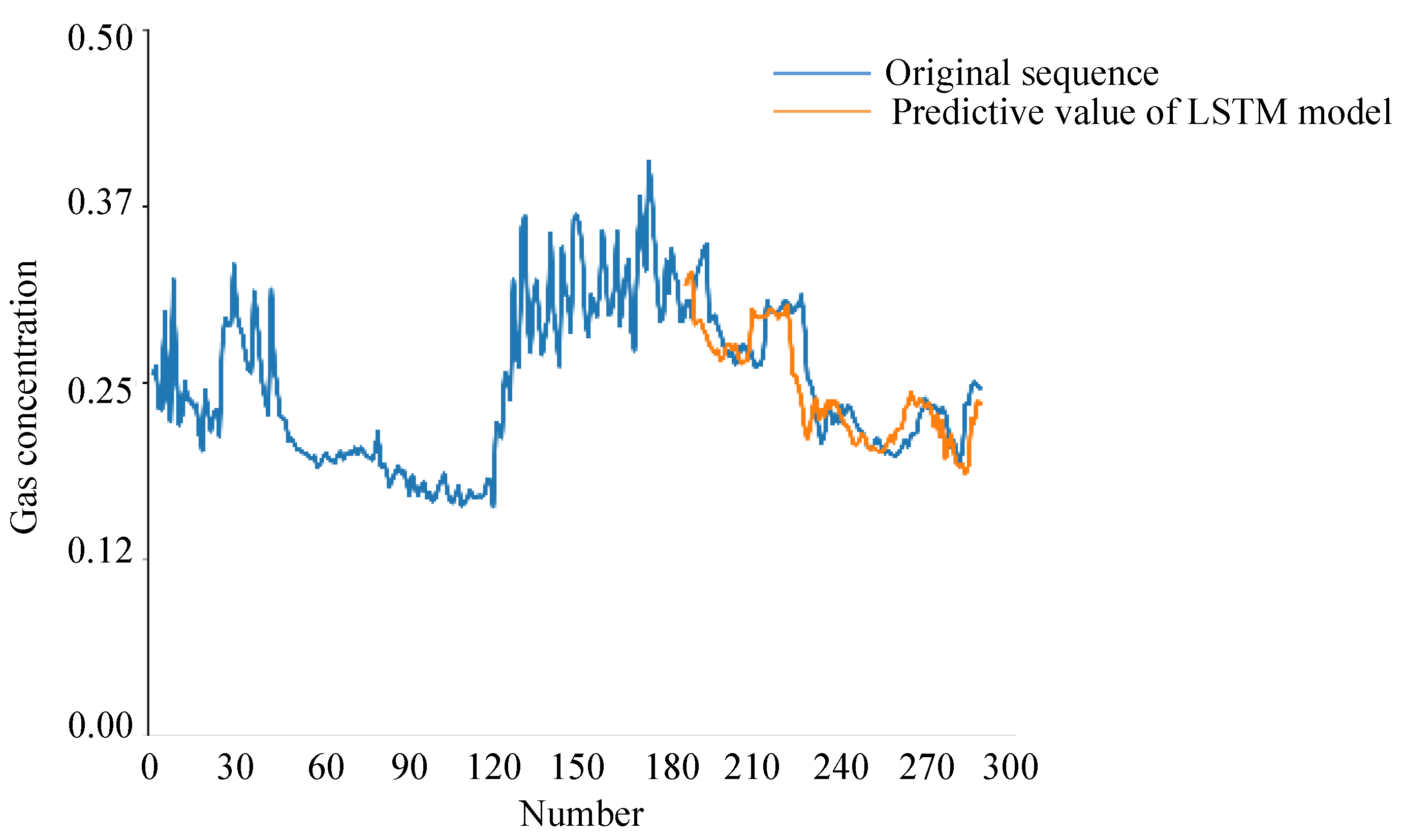
As the ARIMA model and LSTM model have their own advantages in linear and nonlinear models, respectively, the combined ARIMA-LSTM model is proposed. The ARIMA model is used to process the historical data of the gas time series and obtain the corresponding linear prediction results and residual series. LSTM is used for residual data processing and prediction. Finally, the processing results of the two models are superimposed to obtain the final prediction results (Figure 11). In Figure 11, blue is used to show the original data and yellow is used to show the prediction results of the combined ARIMA-LSTM model, from which it can be seen that the prediction curves of the combined model fit well with the original value curves.

4. Discussion

RMSE, MAPE and R2 were used as metrics to evaluate the ARIMA model, LSTM model and combined ARIMA-LSTM model (Table 2). The closer the RMSE and MAPE are to 0, the closer the predicted value is to the observed value, and the closer the R2 value is to 1, the better the fitting effect is. At the same time, combined with the prediction results of each model in Figure 12, the blue line indicates the original gas series, the green line indicates the ARIMA model prediction series, the red line indicates the LSTM model prediction series, and the purple line indicates the ARIMA-LSTM combined model. The combined model, ARIMA-LSTM, is more suitable for gas time series prediction than the single ARIMA model and LSTM model. The ARIMA and LSTM models cannot learn all the patterns of the data, resulting in large errors. The ARIMA-LSTM model is optimal mainly because it learns both linear and nonlinear data features during the training process. However, the causes of errors are related to the interaction of data between different dimensions, in addition to the defects in the model itself. The variation in mine gas concentration is affected by various factors, such as the underground environment and coal mining speed. This paper mainly studies the applicability of the model, and the next step will be to consider prediction under the conditions of various environmental factors.

5. Conclusions

In this paper, the ARIMA model, LSTM model and combined ARIMA-LSTM model are constructed to predict gas concentration data. The optimal model is ARIMA (3,1,0) by combining the autocorrelation function (ACF) and partial autocorrelation function (PACF) with the BIC criterion, and the model’s applicability is tested by Q-Q plots and positive-terrestrial distribution plots. The loss function completely converges when the number of iterations is 30, and the optimal prediction result of the LSTM model is obtained. The ARIMA model is used to process the gas time series data and obtains the corresponding linear forecasts and residual series, while the LSTM model is used to further analyse and predict the nonlinearities in the residual series in the panel data affecting the gas time series and to obtain the final combined model forecasts. The R2 of the ARIMA-LSTM combined model is 0.9825, which is closer to 1 than the other two models, and the RMSE and MAPE values are 0.0830 and 0.0124, respectively, which are closer to 0 than the other two models, resulting in a higher prediction accuracy of the ARIMA-LSTM combined model than the other two models. The combined ARIMA-LSTM model has higher prediction accuracy than the other two models and is more suitable for gas time series prediction, which lays the foundation for intelligent gas hazard prediction and early warning in underground wells.

Author Contributions

Conceptualization, C.L. and X.F. Methodology, C.L., X.F., Z.Y. and Y.H. Validation, C.L., X.F., Z.Y., Y.H. and M.L. Theoretical analysis, C.L. and M.L. Data curation, C.L. Writing—original draft preparation, X.F., Z.Y. and Y.H. Writing—review and editing, C.L. and M.L. Supervision, X.F. Project administration, X.F. All authors have read and agreed to the published version of the manuscript.

Funding

This work was supported by the National Natural Science Foundation of China (Nos. 51874276 and 52004273), the Natural Science Foundation of Jiangsu Province (No. BK20200639).

Data Availability Statement

Data are available in the article.

Acknowledgments

We thank the National Natural Science Foundation of China and the Natural Science Foundation of Jiangsu Province for its support of this study. We thank the academic editors and anonymous reviewers for their kind suggestions and valuable comments.

Conflicts of Interest

The authors declare no conflict of interest.

Abbreviations

ARIMAautoregressive integrated moving average
LSTMlong short-term memory
RNNrecurrent neural network
ACFautocorrelation function
PACFpartial autocorrelation function
BICbayesian information criterion

References

  1. Liang, Y.Q.; Guo, D.Y.; Huang, Z.F.; Jiang, X.H. Prediction model for coal-gas outburst using the genetic projection pursuit method. Int. J. Oil Gas Coal Technol. 2017, 16, 271–282. [Google Scholar] [CrossRef]
  2. Chen, L.; Yu, L.; Ou, J.; Zhou, Y.; Fu, J.; Wang, F. Prediction of coal and gas outburst risk at driving working face based on Bayes discriminant analysis model. Earthq. Struct. 2020, 18, 73–82. [Google Scholar]
  3. Mou, J.; Liu, H.; Zou, Y.; Li, Q. A new method to determine the sensitivity of coal and gas outburst prediction index. Arab. J. Geosci. 2020, 13, 465. [Google Scholar] [CrossRef]
  4. Fu, G.; Zhao, Z.Q.; Hao, C.B.; Wu, Q. The Accident Path of Coal Mine Gas Explosion Based on 24Model: A Case Study of the Ruizhiyuan Gas Explosion Accident. Processes 2019, 7, 73. [Google Scholar] [CrossRef] [Green Version]
  5. Zeng, J.; Li, Q.S. Research on Prediction Accuracy of Coal Mine Gas Emission Based on Grey Prediction Model. Processes 2021, 9, 1147. [Google Scholar] [CrossRef]
  6. Dong, G.; Liang, X.; Wang, Q. A New Method for Predicting Coal and Gas Outbursts. Shock. Vib. 2020, 2020. [Google Scholar] [CrossRef]
  7. Wei, Y.; Chang, J.; Lian, J.; Liu, T. A Coal Mine Multi-Point Fiber Ethylene Gas Concentration Sensor. Photonic Sens. 2015, 5, 67–71. [Google Scholar] [CrossRef] [Green Version]
  8. Tang, J.; Jiang, C.; Chen, Y.; Li, X.; Wang, G.; Yang, D. Line prediction technology for forecasting coal and gas outbursts during coal roadway tunneling. J. Nat. Gas Sci. Eng. 2016, 34, 412–418. [Google Scholar] [CrossRef]
  9. Lu, Z.; Zhu, X.; Wang, H.; Li, Q. Mathematical modeling for intelligent prediction of gas accident number in Chinese coal mines in recent years. J. Intell. Fuzzy Syst. 2018, 35, 2649–2655. [Google Scholar] [CrossRef]
  10. Zhao, B.; Cao, J.; Sun, H.; Wen, G.; Dai, L.; Wang, B. Experimental investigations of stress-gas pressure evolution rules of coal and gas outburst: A case study in Dingji coal mine, China. Energy Sci. Eng. 2020, 8, 61–73. [Google Scholar] [CrossRef] [Green Version]
  11. Wang, Z.-Y. Research on coal mine gas prediction algorithm based on improved Svm. Agro Food Ind. Hi-Tech 2017, 28, 1729–1733. [Google Scholar]
  12. Yu, K.; Qiang, W. Application of ant colony clustering algorithm in coal mine gas accident analysis under the background of big data research. J. Intell. Fuzzy Syst. 2020, 38, 1381–1390. [Google Scholar] [CrossRef]
  13. Xie, C.; Chao, L.; Qin, Y.; Cao, J.; Li, Y. Using a stochastic forest prediction model to predict the hazardous gas concentration in a one-way roadway. Aip Adv. 2020, 10. [Google Scholar] [CrossRef]
  14. Zhang, T.; Song, S.; Li, S.; Ma, L.; Pan, S.; Han, L. Research on Gas Concentration Prediction Models Based on LSTM Multidimensional Time Series. Energies 2019, 12, 161. [Google Scholar] [CrossRef] [Green Version]
  15. Wang, Q.; Li, S.; Li, R.; Ma, M. Forecasting US shale gas monthly production using a hybrid ARIMA and metabolic nonlinear grey model. Energy 2018, 160, 378–387. [Google Scholar] [CrossRef]
  16. Aasim; Singh, S.N.; Mohapatra, A. Repeated wavelet transform based ARIMA model for very short-term wind speed forecasting. Renew. Energy 2019, 136, 758–768. [Google Scholar] [CrossRef]
  17. Wang, C.C.; Chien, C.H.; Trappey, A.J.C. On the Application of ARIMA and LSTM to Predict Order Demand Based on Short Lead Time and On-Time Delivery Requirements. Processes 2021, 9, 1157. [Google Scholar] [CrossRef]
  18. Fan, D.Y.; Sun, H.; Yao, J.; Zhang, K.; Yan, X.; Sun, Z.X. Well production forecasting based on ARIMA-LSTM model considering manual operations. Energy 2021, 220. [Google Scholar] [CrossRef]
  19. Zheng, C.; Deng, J.J.; Hong, Z.X.; Wang, G.H. Prediction Model of Suspension Density in the Dense Medium Separation System Based on LSTM. s. Processes 2020, 8, 976. [Google Scholar] [CrossRef]
  20. Lyu, P.; Chen, N.; Mao, S.; Li, M. LSTM based encoder-decoder for short-term predictions of gas concentration using multi-sensor fusion. Process Saf. Environ. Prot. 2020, 137, 93–105. [Google Scholar] [CrossRef]
  21. Al-Hajj, R.; Assi, A.; Fouad, M.; Mabrouk, E. A Hybrid LSTM-Based Genetic Programming Approach for Short-Term Prediction of Global Solar Radiation Using Weather Data. Processes 2021, 9, 1187. [Google Scholar] [CrossRef]
  22. Zhu, X.X.; Li, L.X.; Liu, J.; Li, Z.Y.; Peng, H.P.; Niu, X.X. Image captioning with triple-attention and stack parallel LSTM. Neurocomputing 2018, 319, 55–65. [Google Scholar] [CrossRef]
  23. Xu, D.H.; Zhang, Q.; Ding, Y.; Zhang, D. Application of a hybrid ARIMA-LSTM model based on the SPEI for drought forecasting. Environ. Sci. Pollut. Res. 2022, 29, 4128–4144. [Google Scholar] [CrossRef] [PubMed]
  24. Wu, X.H.; Zhou, J.Q.; Yu, H.Y.; Liu, D.Y.; Xie, K.; Chen, Y.Q.; Hu, J.B.; Sun, H.Y.; Xing, F.J. The Development of a Hybrid Wavelet-ARIMA-LSTM Model for Precipitation Amounts and Drought Analysis. Atmosphere 2021, 12, 74. [Google Scholar] [CrossRef]
  25. Huang, Y.X.; Fan, J.D.; Yan, Z.G.; Li, S.G.; Wang, Y.P. A Gas Concentration Prediction Method Driven by a Spark Streaming Framework. Energies 2022, 15, 5335. [Google Scholar] [CrossRef]
  26. Abebe, M.; Noh, Y.; Kang, Y.J.; Seo, C.; Kim, D.; Seo, J. Ship trajectory planning for collision avoidance using hybrid ARIMA-LSTM models. Ocean. Eng. 2022, 256. [Google Scholar] [CrossRef]
  27. Xu, P. Prediction of Per Capita Ecological Carrying Capacity Based on ARIMA-LSTM in Tourism Ecological Footprint Big Data. Sci. Program. 2022, 2022. [Google Scholar] [CrossRef]
  28. Manowska, A.; Rybak, A.; Dylong, A.; Pielot, J. Forecasting of Natural Gas Consumption in Poland Based on ARIMA-LSTM Hybrid Model. Energies 2021, 14, 8597. [Google Scholar] [CrossRef]
  29. Huang, Y.X.; Fan, J.D.; Yan, Z.G.; Li, S.G.; Wang, Y.P. Research on Early Warning for Gas Risks at a Working Face Based on Association Rule Mining. Energies 2021, 14, 6889. [Google Scholar] [CrossRef]
  30. Bukhari, A.H.; Raja, M.A.Z.; Sulaiman, M.; Islam, S.; Shoaib, M.; Kumam, P. Fractional Neuro-Sequential ARFIMA-LSTM for Financial Market Forecasting. IEEE Access 2020, 8, 71326–71338. [Google Scholar] [CrossRef]
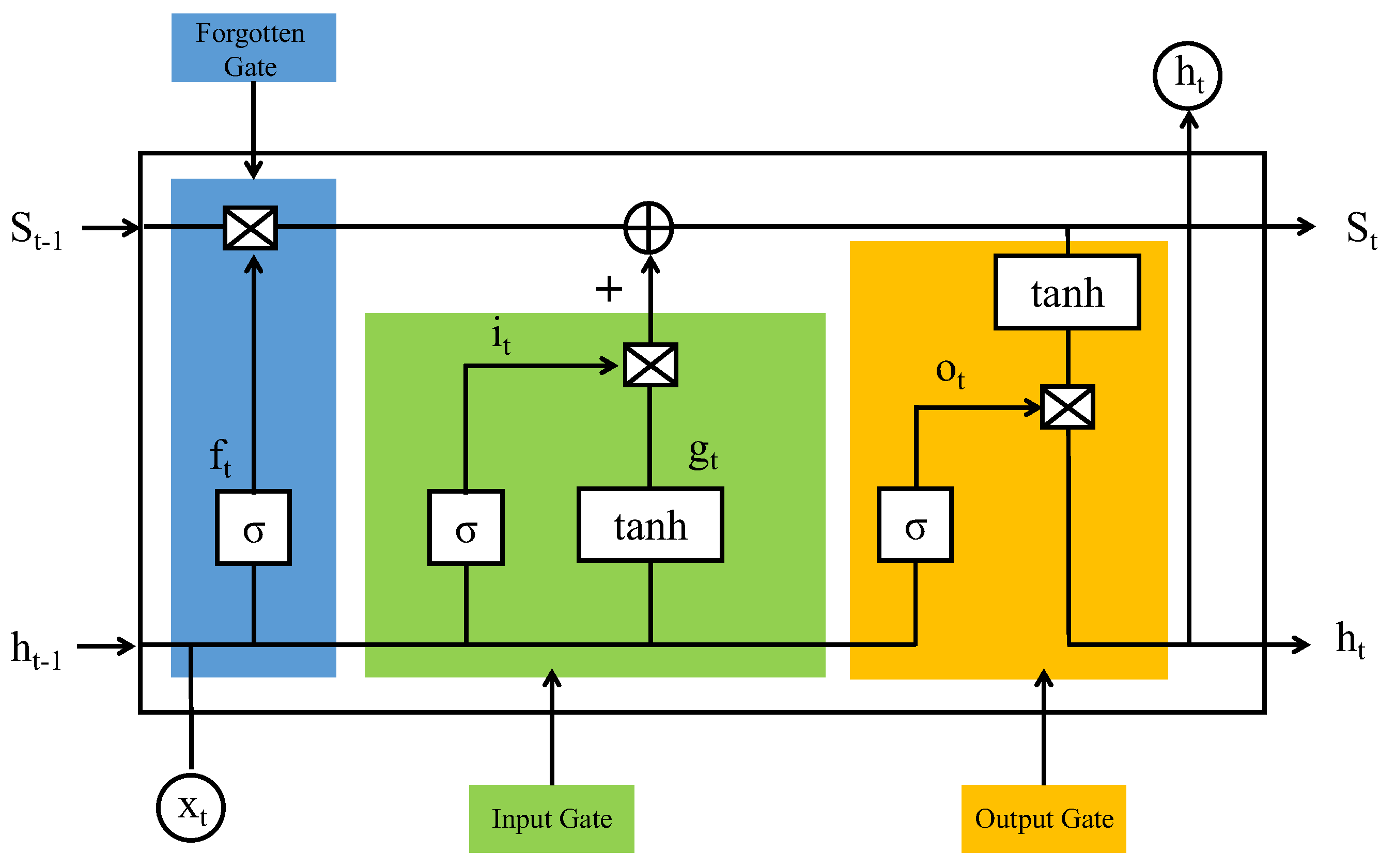
Figure 1. The basic unit of an LSTM network.
Processes 11 00174 g001
Figure 2. Raw gas concentration data.
Processes 11 00174 g002
Figure 3. Postdifferential data sequence.
Processes 11 00174 g003
Figure 4. Autocorrelation function and partial autocorrelation function.
Processes 11 00174 g004
Figure 5. BIC diagram.
Processes 11 00174 g005
Figure 6. Histogram plus estimated density.
Processes 11 00174 g006
Figure 7. Quantile-Quantile plot.
Processes 11 00174 g007
Figure 8. ARIMA model prediction results.
Processes 11 00174 g008
Figure 9. Loss function training process.
Processes 11 00174 g009
Figure 10. LSTM model prediction results.
Processes 11 00174 g010
Figure 11. ARIMA-LSTM model prediction results.
Processes 11 00174 g011
Figure 12. Comparison of prediction results of three models.
Processes 11 00174 g012
Table 1. The augmented Dickey–Fuller test result.
Threshold ValuesPT
1%5%10%0.55−6.32
−2.57−1.94−1.61
Table 2. Table of RMSE, MAPE and R2 evaluation results.
ParametersR2MAPERMSE
ARIMA0.36481.41351.5769
LSTM0.52440.42530.7823
ARIMA-LSTM0.98250.01240.0830
Disclaimer/Publisher’s Note: The statements, opinions and data contained in all publications are solely those of the individual author(s) and contributor(s) and not of MDPI and/or the editor(s). MDPI and/or the editor(s) disclaim responsibility for any injury to people or property resulting from any ideas, methods, instructions or products referred to in the content.