Modelling and Analysis of Dynamic Servo Error of Heavy Vertical Machining Centre Considering Nonlinear Factors

Abstract

The dynamic servo error of heavy-duty vertical machining centres is one of the decisive factors affecting the machining accuracy of large and complex parts. Due to the characteristics of large mass, large load, and the large travel distance of the machine tool, non-linear factors such as friction, backlash, and lateral shift are more likely to cause unstable behaviours such as stick-slip and oscillation of the servo feed system of the machine tool, and reduce the performance and servo accuracy of the motion axis. In this paper, to consider the influence of non-linear factors such as friction, backlash, and lateral shift, an appropriately simplified representation of the mechanical transmission system of the ball screw has been used. According to the control structure of the Siemens 840D numerical control system, a theoretical model of the servo feed system for the heavy-duty vertical machining centre was established based on three-loop control. Then, the single-axis and double-axis closed-loop simulation models of the servo feed system were built in Simulink, and the influence pattern of control parameters and nonlinear factors on the dynamic servo error was obtained through simulation analysis. Finally, the validity of the theoretical model for the servo feed system was verified through a comprehensive comparison of simulation and experimental outcomes. This encompasses an analysis of the control system Bode plots, critical stick-slip velocity, and tracking errors in the X-axis with linear motion. The validation provides theoretical guidance for parameter design and mechanical adjustments of the servo feed system in heavy-duty vertical machining centres.

1. Introduction

Large and complex parts are desired for high growth sectors including railways, aeronautics, and shipping. To cater for the demands for these large parts, the machining accuracy of heavy-duty machine tools of large scale should be guaranteed [1]. However, CNC machine tools are more affected by errors including geometric errors, structural vibration, thermal deformation, and servo dynamic errors [2,3]. Especially in the case of heavy-duty machine tools, with the increased complexity of machining paths, the servo dynamic errors has become one of the dominant factors in determining the machining quality. This is due to the large inertia of the moving parts, the heavy weight of the structural components, and the hard controlled working environment, which is the essential difference when compared to general CNC machine tools. Therefore, how to model and analyse servo dynamic errors of heavy-duty machine tools is the key to the accuracy improvement of large parts from the design perspective of error avoidance.

The dynamic servo error of a machine tool is typically caused by the deviation between the servo motion trajectory and the commanded motion trajectory, which is evaluated as the contour error. This error is induced by the tracking error of each servo axis [4,5]. When there is no tracking error in the servo axes, the multi-axis servo system will not exhibit a contour error. This is due to the fact that the tracking error is mainly affected by the closed-loop control and the hardware/machining conditions such as the static stiffness and the dynamic behaviour of the servo system [6]. In order to study the dynamic servo error of a machine tool, it is first necessary to develop a model of the servo feed system for each motion axis, primarily by modelling the servo drive system and the mechanical transmission system, and then to analyse the resulting characteristics of the servo axis with different factors, and the contour error in multi-axis coordinated motion.

From the published literature, some modelling approaches have been developed. Poo et al. [7,8]. first established the transient and steady-state error equations for two-axis tracking and contour errors. They pointed out that servo closed-loop dynamics between different axes should be tuned to be matched, to improve contouring performance in two-axis control. Based on that concept, a cross-coupled control (CCC) scheme was proposed [9]. The tracking error of each axis is utilized to construct the linear and circular contour error models, and the variable-gain control strategy is used to compensate for contour errors [10]. Many improvements to the CCC were proposed in [11,12,13,14,15,16]. To calculate the real contour errors for free-form curves, real-time contour error estimation algorithms were developed in [15,16]. However, the proposed methods cannot be directly applied to the contour error model and motion control for five-axis motion. This is because the kinematic transformation between the workpiece space and the joint space is nonlinear. Although the contour error model for two or three linear axis controls has been widely investigated in the past, the research area primarily focusses on the contour or dynamic error elimination with the control strategy. This is based on the error compensation concept, not a design approach focusing on error prevention during the design of feed drive systems.

In addition, non-linear factors such as friction and backlash are also important drivers of unstable behaviours such as stick-slip and oscillation of the servo feed system. These lead to contour errors [17]. It can be seen from the experiments in [8] that the current contour error control technologies are unable to eliminate the contour errors caused by these nonlinear factors [18,19]. The contour error caused by nonlinear factors has received widespread attention from scholars in recent years, but research is still in an exploratory state and has not achieved recognized research results [20,21,22]. How to reveal the influence of nonlinear factors on the servo feed system, with modelling and analysis methods, is a fundamental problem. This needs to be solved to prevent dynamic servo errors in machine tools and guide the design of servo systems.

As mentioned above, servo feed drive systems of heavy-duty machining centres consist of two subsystems: the mechanical transmission system and the servo drive system. In practice, the two subsystems are still designed and verified based on analytical equations and experience, respectively. Due to the large inertia of the moving parts, the heavy weight of structural components and the hard controlled environment, the factors that affect the performance of feed drive systems become complicated. The dynamic modelling of servo errors in heavy-duty vertical machining centres is currently beset with the following issues:

(1)

The mechanical transmission system model is derived based on the modelling approach used for conventional CNC machine tools. These models represent the mechanical transmission simply using a second-order model, ignoring the change of stiffness caused by the large distances travelled, and the long transmission chains of the heavy-duty machine tools. At the same time, the non-linear change in friction caused by the change of oil film thickness in the hydrostatic guideway, due to the large inertia and large load of the heavy-duty machine tool, is ignored.

(2)

The modelling of the servo drive system is often ignored, and the classic PID is used for the error model. This results in a situation where the theoretical model does not match the actual machine tool behaviour. The error model formulated in this scenario will consequently result in imprecise analysis of error-inducing factors, thereby complicating the provision of theoretical guidance for effectively reducing errors in heavy machine tools.

In this paper, to accurately investigate the performance of the feed drive systems for a heavy-duty machining centre, a mechatronics model of the servo feed drive system is established. This allows an examination of how the parameters affect the dynamic errors. The mechanical transmission subsystem is simplified and modelled taking the characteristics of heavy-duty machining centres and nonlinear factors into account. The model is then utilized to evaluate the dynamic servo errors with different feed rates or paths of linear servo axes using simulations. The validity of the theoretical model for the servo feed system is verified through a comprehensive comparison of simulation and experimental outcomes. This encompasses the analysis of control system Bode plots, critical stick-slip velocity, and tracking errors of a single servo axis with linear motion.

This paper is arranged as follows: Section 1, this section, is the introduction. Section 2 covers the modelling of the servo feed system of a heavy-duty vertical machining centre. In Section 3, the developed model is employed to analyse the factors that influence the dynamic servo error in the context of the heavy-duty vertical machining centre. The last section demonstrates the experimental verification of the servo feed system of the heavy-duty vertical machining centre, the critical stick-slip velocity and the tracking error of the servo axis with linear motions.

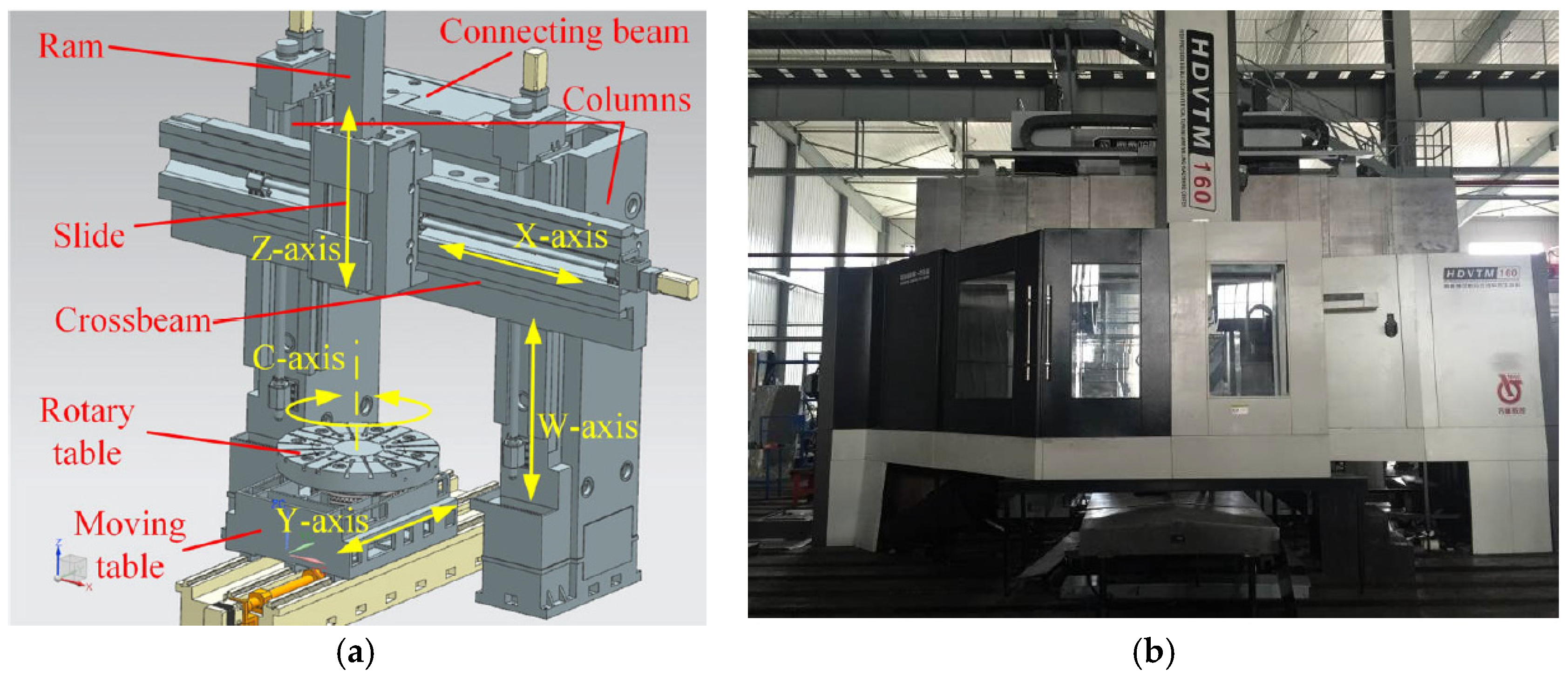
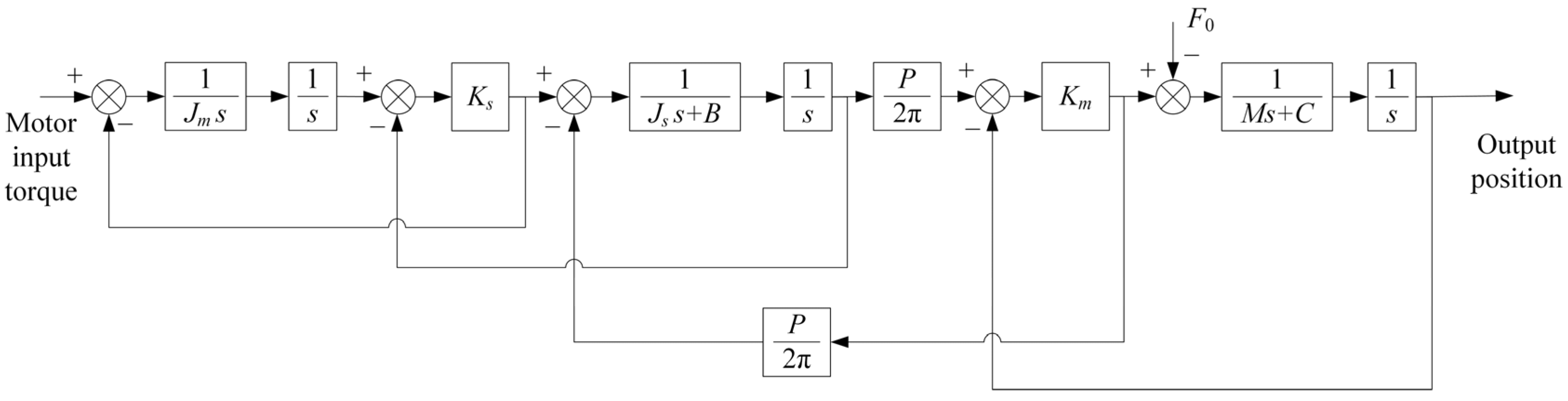
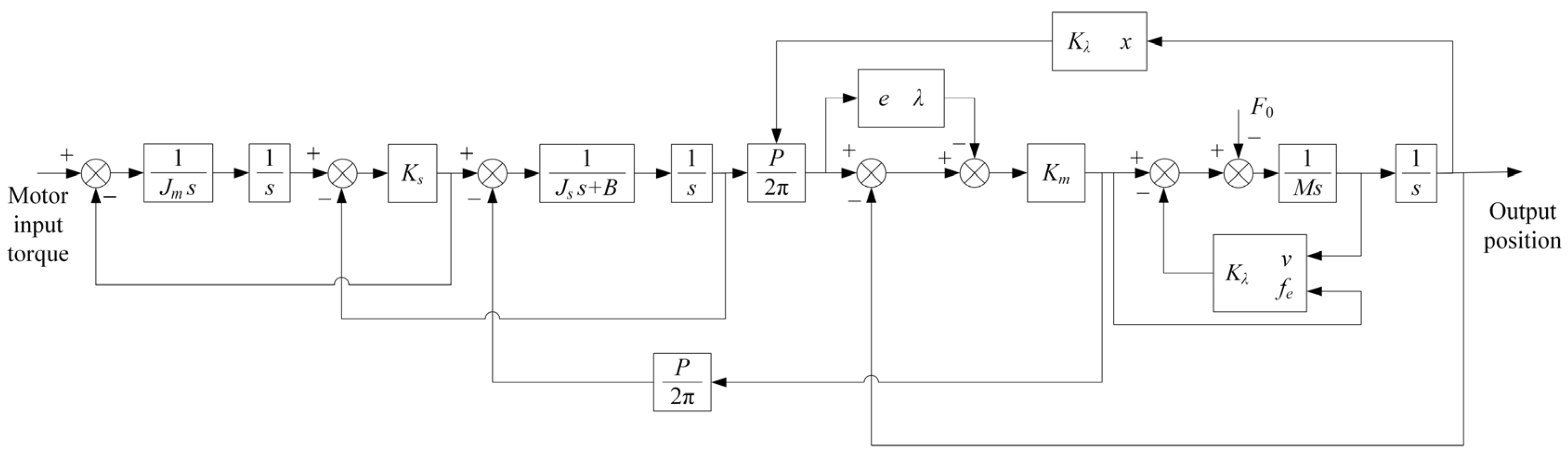
2. Modelling of the Servo Feed System in a Heavy-Duty Vertical Machining Centre

The research focus of this article is a heavy-duty vertical machining centre with a maximum machining diameter of Φ1600 mm and a maximum machining weight of 8 tonnes. The feed rate ranges for the X and Y axes are 0.1 to 1000 mm/min. The servo feed system uses a ball screw transmission, and the driving system is based on the Siemens 840D CNC system, with a 611D driver. The physical machine tool is shown in Figure 1.

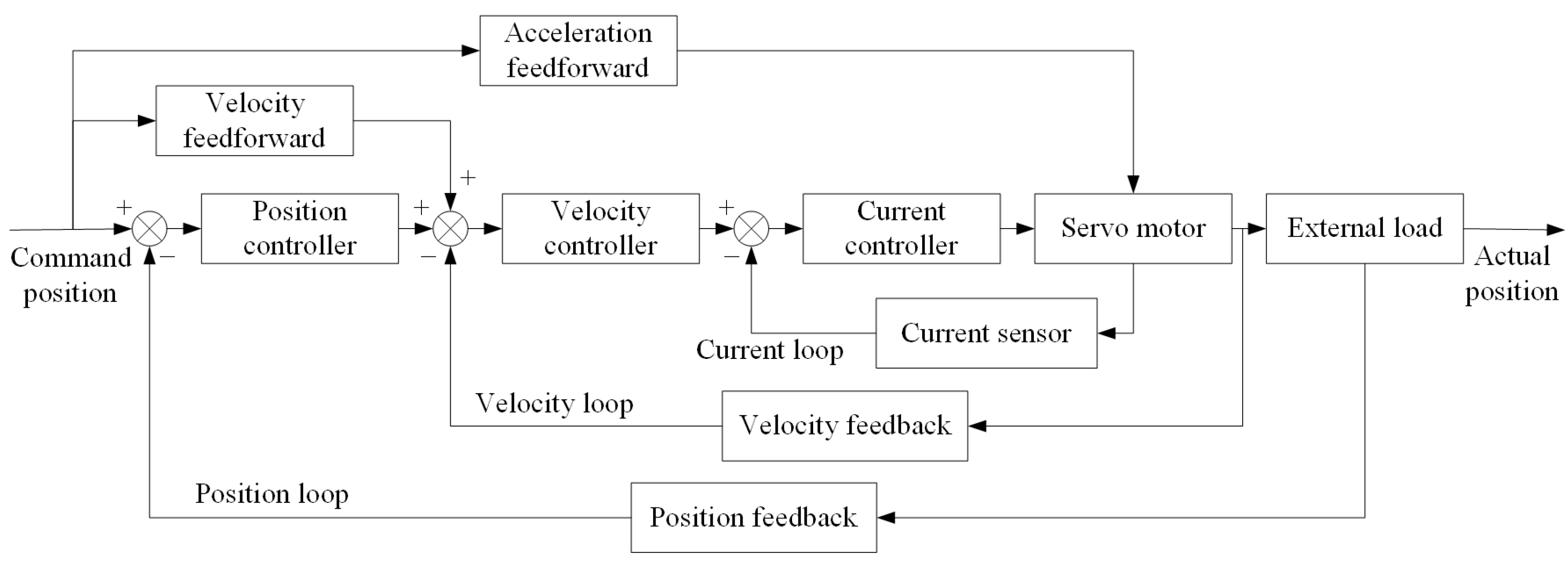
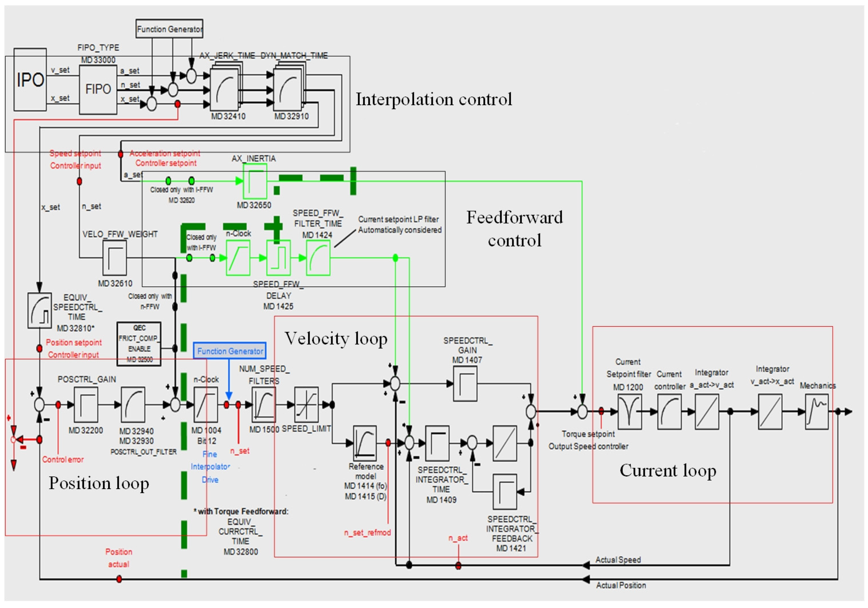
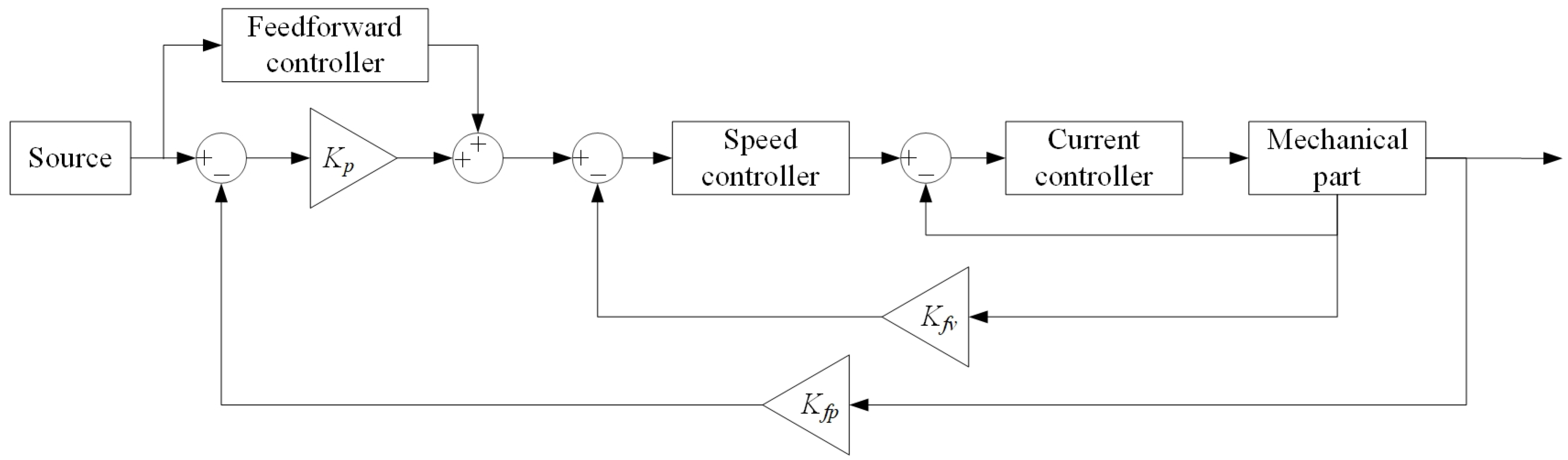
2.1. Development of a Theoretical Model of a Servo Drive System

At present, the control structure of numerically controlled systems mostly adopts a three-loop control structure, consisting of a current loop, a velocity loop, and a position loop, as shown in Figure 2. The current loop is the innermost loop, the velocity loop is the middle loop and the position loop is the outermost loop. The purpose of the current loop is to ensure the rapid response of the output current, so that the system can run quickly, and at the same time suppress the influence of external disturbances; the function of the velocity loop is to ensure stable actual velocity according to the velocity command, so that the entire system can run stably; the position loop is to guarantee the accuracy and tracking performance of the actual position so that the entire servo control system can run stably.

The CNC system used in the heavy-duty vertical machining centre studied in this project is the Siemens 840D control system. The 840D uses the three-loop control structure, Figure 3 shows the framework. This framework is commonly used in many commercial CNC systems, such as FANUC, HEIDENHAIN, and so on. The parameters and conversion coefficients in the realistic CNC system, which determine the parameter values in the simulation model, might differ according to different CNC systems. Thus, the theoretical servo control model that can be built based on this structure has certain universality.

(1)

Mathematical model of the current loop

The current loop generally adopts a PI controller, which is mainly composed of a servo motor, a driver, and a controller. The specific structure diagram is shown in Figure 4, without considering the differential and limiting blocks in the current controller.

Based on the characteristics of the PI controller, the transfer function of the current controller can be obtained as:

$$G_i=K_i(\frac{T_{i}s+1}{T_{i}s}),$$

(1)

where K_i is the proportional gain of the current loop and T_i is the integral time constant of the current loop. In engineering applications, the two variables are often represented by the expression of integral gain τ_i = K_i/T_i.

In Figure 4, T_cf is the time constant of filtering of the forward pass. For simplification, the feedback current also adopts the same filtering time constant. The filter selection depends on the application of the numerical control system; R_a is the equivalent armature winding resistance, L_a is the equivalent armature inductance, K_e is the back electromotive force coefficient, and K_t is the torque current coefficient. These parameters can be found on the motor nameplate. K_a is the current feedback coefficient, and normally it is set to 1.

(2)

Mathematical model of the velocity loops

The velocity loop typically employs a PI controller, and its main components are a servo motor, a velocity controller, and a filter. The servo motor uses a Siemens FT1605 permanent magnet synchronous motor. Derived from the breakdown of the elements within the velocity loop, the configuration of the velocity loop is illustrated in Figure 5.

In Figure 5, K_t is the torque current constant, the units are N/A; J_m is the equivalent moment of inertia of the motor rotor, the units are kg∙m²; B is the equivalent damping coefficient of the motor rotor; K_b is the velocity feedback coefficient, which is usually taken as 1.

The transfer function of the velocity controller is:

$$G_{sc}(s)=K_s(\frac{T_{s}s+1}{T_{s}s}),$$

(2)

where K_s is the proportional gain of the velocity loop and T_s is the integral time constant of the velocity loop. In engineering applications, the two variables are often combined as the integral gain τ_s = K_s/T_s.

(3)

Mathematical model of the position loop

The position loop uses a position controller to generate velocity commands by differencing the commanded position and the feedback position of the grating ruler, which serves as the input signal to the velocity loop. Based on common practice, it generally uses a proportional gain controller.

A position loop includes a position controller, velocity loop, load, velocity feedforward, acceleration feedforward, and so on. Velocity feedforward and acceleration feedforward mainly ensure that the position loop can accurately follow the command signal if velocity or acceleration signals are the input. The position feedback generally has a grating ruler, including information detection, information transmission, information recognition. If complex information processing is involved, it can be regarded as a proportional block with a transfer function G(s) = K_ϕ = 1. Utilizing the preceding analysis, the control structure of the position loop is depicted in Figure 6.

In Figure 6, K_p is the proportional gain of the position loop; G_f(s) and G_ff(s) are the transfer functions of velocity feedforward and acceleration feedforward, respectively; G_b(s) is the transfer function of the velocity loop. G_m(s) is the transfer function of the mechanical transmission system.

In practical systems, both velocity feedforward and acceleration feedforward can be derived with transfer functions. The transfer function of the velocity feedforward is:

$$G_f(s)=k_{f}s.$$

(3)

Transfer function of acceleration feedforward is:

$$G_{ff}(s)=I\cdot s^2,$$

(4)

where k_f and I are the velocity and acceleration feedforward coefficients.

Within the servo control system, the principal control performance of the position loop requires that on one hand, the tracking error should be small in the steady state position; on the other hand, the process should be smooth when the steady state error is reached. Therefore, it is necessary to constantly adjust the controller to select the appropriate servo gain coefficient and feedforward coefficient.

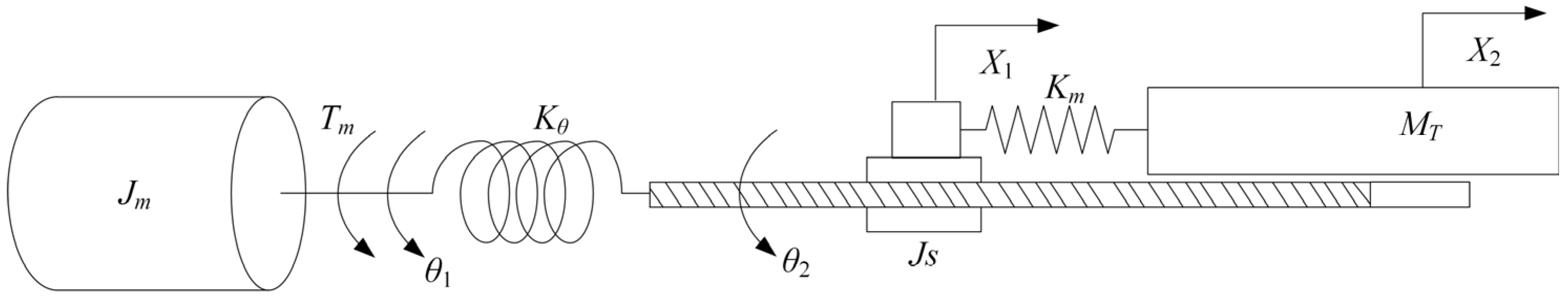
2.2. Development of the Theoretical Model of the Mechanical Transmission System

2.2.1. Modelling of Ball Screw Transmission

Taking the X-axis as an example, the ball screw transmission system of the heavy-duty vertical machining centre is developed, which includes the controller, servo motor, coupling, grating ruler, driver, screw, bearing group, worktable, guide rail, and other components, as demonstrated in Figure 7.

For the modelling of a transmission system, the most commonly used method for the ball screw transmission is to equivalently convert the transmission stiffness, damping, moment of inertia, and other attributes of other parts of the drive chain to the ball screw. Then, using the physical model of the motor driving the screw’s rotation, the corresponding dynamic equations are obtained [24]. This traditional modelling approach is more suitable for small-sized machine tools. However, for heavy-duty machine tools, their large travel distance and long transmission chain can cause stiffness to vary with displacement. The massive beam and large span can lead to deformations, thereby affecting the screw’s deflection. Additionally, the heavy workload and significant variation in cutting forces can cause changes in the oil film thickness, resulting in changes in the contact surface stiffness. Therefore, to model transmission systems in heavy-duty machine tools, a more comprehensive modelling approach should be created, taking into account each potential factor that may affect its motion precision.

Taking the structure shown in Figure 7 as an example, it is possible to make a reasonable simplification of the transmission system. On one hand, the torsional stiffness of the entire transmission chain is equivalently converted to the coupling. On the other hand, the connection stiffness of the entire transmission chain is equivalently converted to the connection between the screw-nut pair and the worktable. Therefore, the screw feed system can be simplified into an equivalent dynamic model as shown in Figure 8.

In Figure 8, K_θ represents the comprehensive torsional stiffness at the coupling and K_m represents the comprehensive connection stiffness between the screw-nut pair and the worktable. Based on the transmission, the dynamic equation of the mechanical transmission system can be derived as follows:

$$J_m\frac{d^2{\theta }_1}{d{t}^2}=T_m-K_{\theta }(i_t{\theta }_1-{\theta }_2)$$

(5)

$$J_s\frac{d^2{\theta }_2}{d{t}^2}+B\frac{d{\theta }_2}{dt}=K_{\theta }(i_t{\theta }_1-{\theta }_2)-\frac{P}{2\pi }{K}_m(X_1-X_2)$$

(6)

$$M_T\frac{d^2{X}_2}{d{t}^2}+C\frac{d{X}_2}{dt}=K_m(X_1-X_2),$$

(7)

where X₁ = θ₂·P/2π;

J_m  

is the total converted moment of inertia of the motor rotor, coupling and gear reducer (kg∙m²);

T_m 

is the torque output by the motor (N·m);

θ₁  

is the rotation angle of the gearbox output shaft (rad);

θ₂  

is the rotation angle of the ball screw (rad);

i_t    

is the transmission ratio of the gear reducer;

X₁  

is the converted translational displacement of the lead screw (m);

X₂  

is the displacement of the worktable (m);

J_s    

is the total moment of inertia at one end of the ball screw and coupling (kg∙m²);

M_T 

is the total mass of the worktable and screw nut (kg);

P    

is the pitch of the ball screw (m);

K_θ  

is the comprehensive torsional stiffness (N·m/rad);

K_m  

is the comprehensive connection stiffness (N/m).

Normally, the comprehensive torsional stiffness K_θ can be calculated theoretically. In this transmission system, the main components to consider for torsional stiffness are the ball screw and the coupling. The calculation formula is given in Equation (8)

$$\frac{1}{K_{\theta }}=\frac{1}{K_{screw\theta }}+\frac{1}{K_{coup\theta }},$$

(8)

where K_screwθ is the torsional stiffness of the ball screw (N·m/rad);

K_coupθ is the torsional stiffness of the coupling (N·m/rad).

Similarly, when evaluating the comprehensive connection stiffness K_m, it is necessary to take into account factors such as the axial stiffness of the screw-nut pair, the axial stiffness of the ball screw, the stiffness of the bearings, and the contact stiffness at the mating surfaces. In this paper, to ensure sufficient stiffness for heavy-duty machine tools, the bearing block stiffness K_BQ and the nut block stiffness K_NR can be assumed to be sufficiently large, and then their deformations can be neglected. Therefore, the main factors to consider for the calculation of K_m are the axial stiffness of the screw-nut pair, the axial stiffness of the ball screw, the axial stiffness of the bearings, and the contact stiffness at the mating surfaces. The relationship of these parameters is given in Equation (9)

$$\frac{1}{K_m}=(\frac{1}{K_{coupS}}+\frac{1}{K_{screwS}}+\frac{1}{K_{bearS}}+\frac{1}{K_{joinS}}),$$

(9)

where

K_coupS  

the axial stiffness of the screw-nut pair (N/m);

K_screwS 

the axial stiffness of the ball screw (N/m);

K_bearS   

the axial stiffness of the bearings (N/m);

K_joinS    

the contact stiffness at the mating surfaces (N/m).

Without considering nonlinear blocks, the Simulink block diagram for the mechanical transmission is shown in Figure 9.

The heavy-duty vertical machining centre is characterized by its large mass, heavy loads, long travel distance, and significant inertia. Therefore, both linear and nonlinear elements need to be considered for the modelling of mechanical transmission. Friction, backlash, and lateral shift are typical examples of nonlinear elements that must be considered for the analysis of the servo system’s tracking error.

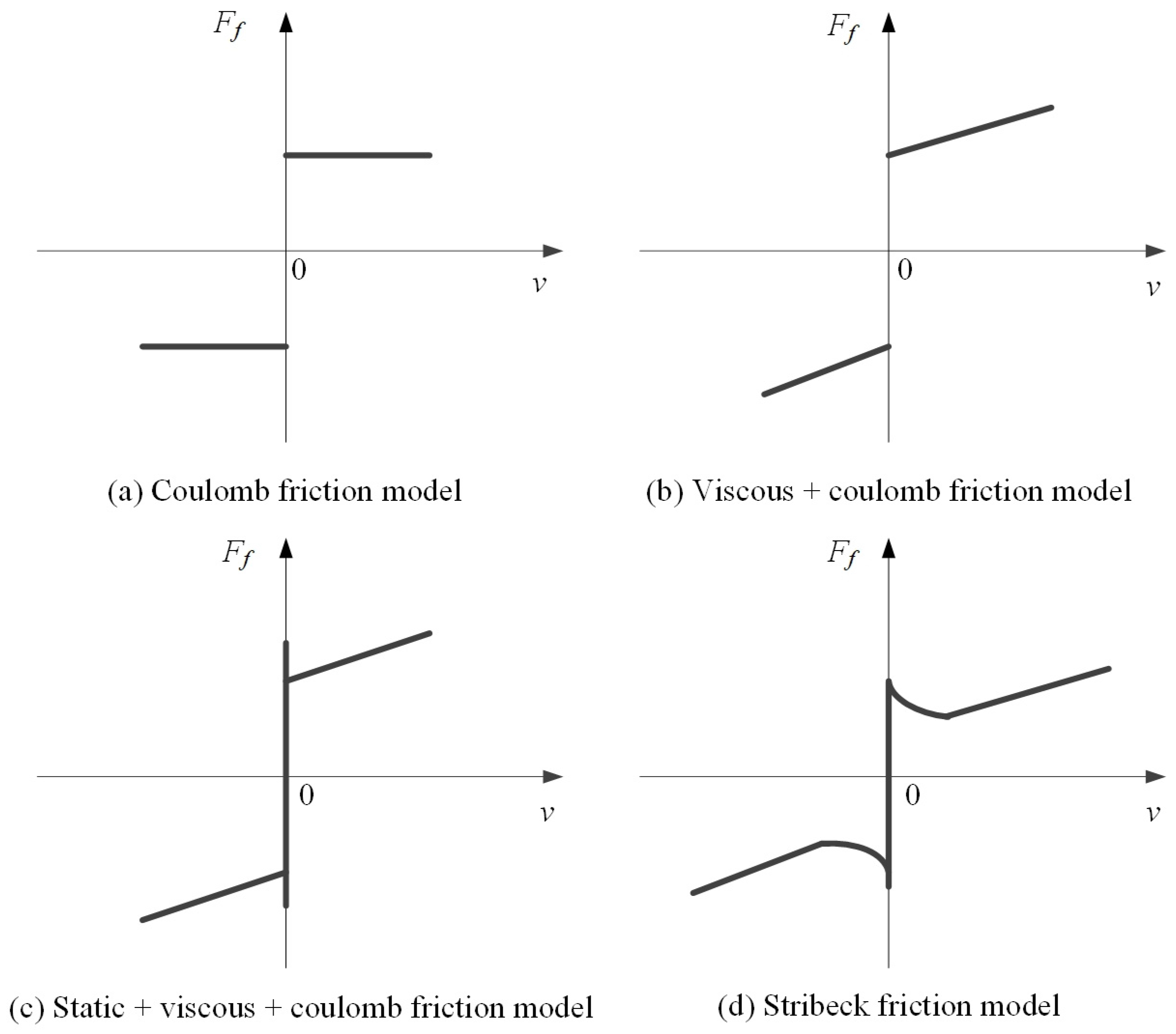
2.2.2. Modelling of Friction

For heavy-duty machine tools, the magnitude of frictional force directly affects the dynamic performance of the entire servo system. Hence, it becomes imperative to incorporate frictional force as a disruptive model. Presently, within the majority of engineering applications, frictional force is often approached as a static force. There are four main types of static friction models, as shown in Figure 10.

Considering that heavy-duty machine tools often operate at low speed with heavy load, stick-slip phenomenon is likely to occur. This indicates that frictional forces experience frequent abrupt changes at low speeds. Therefore, this paper adopts a friction model that includes static friction, viscous friction, and Coulomb friction. The equation for the frictional force is as follows

$$F_f=\{\begin{array}{l}{f}_e\hspace{0.17em}\hspace{0.17em}\hspace{0.17em}\hspace{0.17em}\hspace{0.17em}\hspace{0.17em}\hspace{0.17em}\hspace{0.17em}\hspace{0.17em}\hspace{0.17em}\hspace{0.17em}\hspace{0.17em}\hspace{0.17em}\hspace{0.17em}\hspace{0.17em}\hspace{0.17em}if\hspace{0.17em}v=0\hspace{0.17em}and\hspace{0.17em}\left|f_e\right|<f_s\\ f_s\cdot sgn(f_e)\hspace{0.17em}\hspace{0.17em}\hspace{0.17em}\hspace{0.17em}\hspace{0.17em}\hspace{0.17em}\hspace{0.17em}if\hspace{0.17em}v=0\hspace{0.17em}and\hspace{0.17em}\left|f_e\right|\ge f_s\\ f_v+f_c\cdot sgn(v)\hspace{0.17em}\hspace{0.17em}\hspace{0.17em}\hspace{0.17em}\hspace{0.17em}\hspace{0.17em}\hspace{0.17em}\hspace{0.17em}\hspace{0.17em}\hspace{0.17em}\hspace{0.17em}\hspace{0.17em}\hspace{0.17em}\hspace{0.17em}\hspace{0.17em}if\hspace{0.17em}v\ne 0\end{array},$$

(10)

where

• f_v is the viscous friction coefficient (N∙s/m);
• f_e is the external force (N);
• f_s is the maximum static friction force (N);
• f_c is the Coulomb friction force (N).

If the velocity (v) is zero, the friction force equals the external driving force. Only when the driving force is greater than the maximum static friction force can the moving components be set in motion. When the velocity (v) changes from zero to a non-zero value, the friction force undergoes an abrupt change, transitioning from the maximum static friction force to the Coulomb friction force. If the velocity (v) is non-zero, the friction force becomes a continuous value, increasing with the increase of velocity.

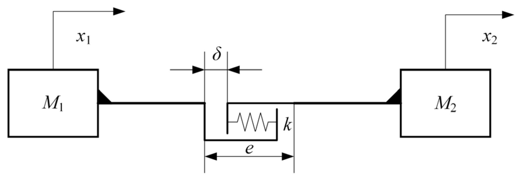
2.2.3. Modelling of Backlash

In CNC machine tools, the backlash happens when the feed mechanism experiences an empty travel as it undergoes a direction change, which is caused by the presence of clearance in the transmission chain. In heavy-duty machine tools, the backlash primarily exists on the transmission ball screw, so it can be approximately considered that the clearance in the ball screw represents the clearance in the transmission chain.

The simplified model of a one-dimensional transmission mechanism with backlash in the ball screw transmission system is illustrated in Figure 11. In the figure, M₁ represents the mass of the input, M₂ represents the mass of the output, there is a transmission clearance e, δ denotes relative displacement offset, and k_m is the contact stiffness when M₁ and M₂ come into contact, which is the same value as the connection stiffness mentioned in the modelling of the mechanical transmission.

From Figure 11, it can be observed that:

$$\delta =x_2-x_1.$$

(11)

The transmission induced contact deformation Δ between M₁ and M₂ is:

$$\Delta =\{\begin{array}{l}\left|\delta \right|-e\hspace{0.17em}\hspace{0.17em}\hspace{0.17em}\hspace{0.17em}\hspace{0.17em}\hspace{0.17em}\left|\delta \right|-e\hspace{0.17em}>0\\ 0\hspace{0.17em}\hspace{0.17em}\hspace{0.17em}\hspace{0.17em}\hspace{0.17em}\hspace{0.17em}\hspace{0.17em}\hspace{0.17em}\hspace{0.17em}\hspace{0.17em}\hspace{0.17em}\left|\delta \right|-e\hspace{0.17em}\le 0\end{array}.$$

(12)

The contact force F is:

$$F=\{\begin{array}{cc}k\Delta \cdot sgn\left(\delta \right)& \Delta >0\\ 0& \Delta \le 0\end{array}.$$

(13)

According to Newton’s law, the relationship can be expressed as in Equation (14):

$$M_2{\ddot{x}}_2=k_m\delta -k_m\lambda \cdot sgn\left(\delta \right),$$

(14)

where $\lambda =\{\begin{array}{l}|\delta |,\hspace{0.17em}\hspace{0.17em}\hspace{0.17em}\hspace{0.17em}\hspace{0.17em}\hspace{0.17em}|\delta |\le e\\ e,\hspace{0.17em}\hspace{0.17em}\hspace{0.17em}\hspace{0.17em}\hspace{0.17em}\hspace{0.17em}\hspace{0.17em}|\delta |>e\end{array}\hspace{0.17em}$.

Equation (14) can be regarded as a superposition of a linear system and a nonlinear system, where the nonlinear system is unstable. As the backlash in the ball screw is usually small, its impact on the whole system is limited but should not be ignored. From the analysis, it is evident that the backlash in the ball screw can cause oscillations in the output of the system, and the amplitude of the oscillations is directly related to the magnitude of the backlash in the ball screw.

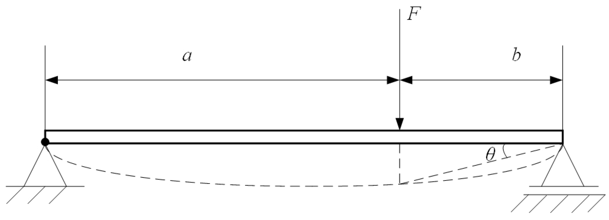
2.2.4. Lateral Shift Model

For heavy-duty machine tools, the gravitational deformation caused by the large mass of moving components cannot be ignored. Therefore, it is necessary to consider its impact on the transmission system. In this section, taking the X-axis of the machine tool, which includes the beam-slide-tool holder feed system, as an example, the effect of the lateral shift caused by the gravitational deformation of the beam and its moving components on the servo transmission system is analysed. The ball screw is fixed at the two ends of the beam. If the beam undergoes deformation, each point of the ball screw will have lateral shifts. In this study, the beam is considered to be simply supported. The force and deformation of the beam are shown in Figure 12.

In the diagram, F is the force exerted by the tool holder on the beam, a is the distance from the tool holder to the left end of the beam, b is the distance from the tool holder to the right end of the beam, and θ is the angle between the line connecting the actual tool holder’s position to one end of the beam and the horizontal line. The expression of the beam’s deflection is given in Equation (15).

$$y_x=\{\begin{array}{l}\frac{Fbx}{6lEI}[l^2-b^2-x^2]\hspace{0.17em}\hspace{0.17em}\hspace{0.17em}\hspace{0.17em}\hspace{0.17em}\hspace{0.17em}\hspace{0.17em}\hspace{0.17em}\hspace{0.17em}\hspace{0.17em}\hspace{0.17em}\hspace{0.17em}\hspace{0.17em}\hspace{0.17em}\hspace{0.17em}\hspace{0.17em}\hspace{0.17em}\hspace{0.17em}\hspace{0.17em}\hspace{0.17em}\hspace{0.17em}\hspace{0.17em}\hspace{0.17em}0\le x\le a\\ \frac{Fb}{6lEI}[\frac{l}{b}{(x-a)}^2-x^3+(l^2-b^2)x]\hspace{0.17em}\hspace{0.17em}\hspace{0.17em}\hspace{0.17em}\hspace{0.17em}\hspace{0.17em}a<x\le a+b\end{array},$$

(15)

where y_x is the deflection of the beam (m);

F   

is the gravitational force exerted by the tool holder, ram, and slide (N);

EI 

is the bending stiffness of the beam (N/m);

l    

is the total length of the beam (m);

x   

is the distance from the calculation point to the left end of the beam (m).

The shift of the ball screw at the tool holder position (x = a) is considered by multiplying the ball screw’s pitch by a lateral shift coefficient. The calculation formula for the shift coefficient is as follows:

$$K_{\lambda }=\cos (\theta )\hspace{0.17em}=\frac{b}{\sqrt{b^2+y_a^2}}.$$

(16)

By incorporating the friction model, backlash model, and lateral shift model as disturbance inputs into the mechanical transmission block diagram shown in Figure 9, the complete diagram of the whole mechanical system is obtained, as shown in Figure 13. As this model is established based on the characteristics of heavy-duty machine tools, it is closer to the actual engineering conditions and holds certain engineering significance.

3. Analysis of the Factors Influencing Servo Error in Heavy-Duty Vertical Machining Centres

The servo error refers to the difference between the CNC command and the real-time actual position of the motion axis. This difference arises due to tracking errors in the servo axis, stemming from both the control system and the mechanical system. In the previous section, a theoretical model of the servo feed system with disturbance factors is developed based on the characteristics of heavy-duty vertical machining centres. In this section, the single-axis simulation model is built for the servo feed system in Simulink, and then the simulation results are used to identify and analyse the main factors that affect the tracking error of the servo axis.

3.1. Simulation Module of a Closed-Loop Servo Feed System

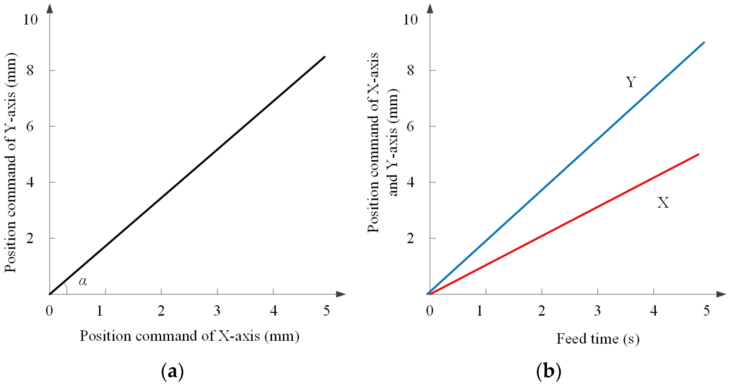
3.1.1. Input Command Design

If the feed rates of the X and Y axes of a heavy-duty vertical machining centre are denoted as F_x and F_y, and the tool tip positions are represented as x_c(t) and y_c(t), respectively, then the input command for a linear trajectory can be expressed as follows:

$$\{\begin{array}{l}{x}_c(t)=F_{x}t=Ft\cos \alpha \\ y_c(t)=F_{y}t=Ft\sin \alpha \end{array}$$

(17)

If the feed rate F = 120 mm/min and the angle α = 60°, then the commands for the X and Y axes are given as shown in Figure 14.

In Simulink, the mathematical expressions of the dual-axis linear input signals are depicted in Figure 15. This model can be used as a signal source for the subsequent simulations described in the following sections.

3.1.2. Simulation Model of Servo Feed System

From Figure 13, it can be seen that, if all the models in the servo system are placed in Simulink, it will make the entire system look very messy and not conducive to analysis. To make the whole model look concise, Subsystem is used to modularize each part in Simulink. As a result, a single-axis closed-loop servo feed system model is obtained, as shown in Figure 16.

3.2. Simulation and Analysis of Factors Affecting Servo Error

3.2.1. Simulation and Analysis of Nonlinear Factors

The simulation parameters for a vertical lathe/milling multi-task machine are summarised in

Table 1. Simulation parameters table.

Parameter	Value	Parameter	Value
Position loop gain Kp (rad/s/m)	26.18 × 103	Current loop gain Ki (V/A)	18.431
Position feedback coefficient Kϕ	1	Current loop integral time constant Ti (s)	0.002
Feedforward coefficient kf	1	Total rotational inertia of motor rotor and shaft sleeve Jm (kg·m2)	0.0215
Equivalent inertia of X-axis Ix (kg·m2)	0	Torsional stiffness of the elastic body between the two sleeves of the coupling Kθ (N·m·rad−1)	4 × 107
Velocity loop gain Ks (A·s·rad−1)	6.84
Velocity loop feedback coefficient Kb	1	The total rotational inertia of the ball screw and its shaft sleeve Js (kg·m2)	0.010
Velocity loop time constant Ts (s)	0.01	Ball screw lead (m)	0.016
Motor winding resistance (Ω)	0.22	Equivalent connection stiffness between screw nut and ball screw Km (kg·m2)	3.6 × 108
Motor armature inductance (H)	4.7 × 10−3	Total mass of worktable and screw MT (kg)	6000
Torque current coefficient (N·m·A−1)	2.34	Transmission ratio itx	0.25

.

In Simulink, using the X-axis as an example, the simulation parameters are applied. It is established that under the default conditions, the linear trajectory input signal is a ramp signal with a feed rate of 500 mm/min, and the circular arc trajectory input signal is a sine curve with a feed rate of 1000 mm/min and a radius of 300 mm.

It is noted that the units of simulation parameters are not consistent with the units in the actual NC system. After conversion, the control parameters of the actual CNC system and simulation are summarized in

Table 2. CNC system and simulation model servo control parameters.

	Current Loop		Velocity Loop		Position Loop
	Proportional Gain	Integral Time Constant	Proportional Gain	Integral Time Constant	Proportional Gain
Numerical Control system	18.14 V/A	2 ms	16 N∙m∙s/rad	10 ms	1 m/min/mm
Simulation Model	18.14 V/A	2 ms	6.84 N∙m∙s/rad	10 ms	26.18 rad/s/mm

.

(1)

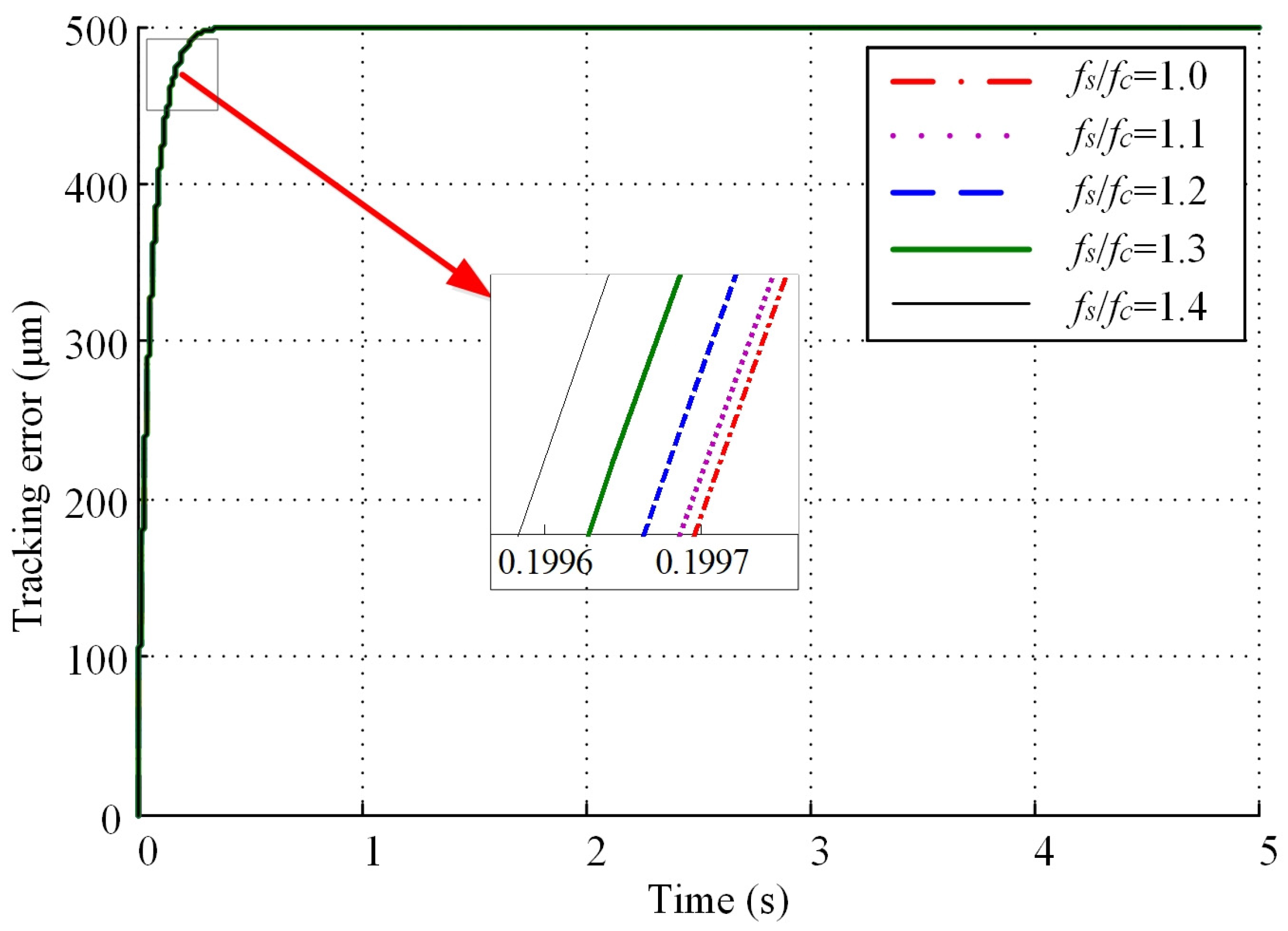
The effects of friction force on tracking error

In the model of the heavy-duty vertical machining centre, frictional force is the most significant disturbance, hence it has the most substantial effect on the tracking error. From the friction force model given in Equation (10), which includes static friction, Coulomb friction (sliding friction), and viscous friction, there are three factors that determine the friction force curve: maximum static friction force (f_s), Coulomb friction force (f_c), and viscous friction coefficient (f_v). The three factors can be quantified to the following three variables: static-to-dynamic friction ratio (f_s/f_c), Coulomb friction coefficient (c), and viscous friction coefficient (f_v) [25].

For the single axis, with other simulation parameters kept constant, the static-to-dynamic friction ratio (f_s/f_c) is sequentially changed to 1.0, 1.1, 1.2, 1.3, and 1.4. The simulation results for different static-to-dynamic friction ratios are shown in Figure 17. It can be seen that the change in the static-to-dynamic friction ratio has little effect on the tracking error in the stable state. The significant effect is observed during machine tool startup. The larger the static-to-dynamic friction ratio, the greater the startup tracking error, and the longer the startup time.

For the single axis, with other simulation parameters kept constant, the Coulomb friction coefficient (c) is sequentially changed to 0.01, 0.02, 0.03, 0.04, and 0.05. The simulation results for the different Coulomb friction coefficient values are shown in Figure 18. It can be observed that the variation in the Coulomb friction coefficient has little effect on the steady-state tracking error. The significant effect is observed during machine tool startup, where a higher Coulomb friction coefficient leads to a larger startup tracking error and a longer startup time. The larger the Coulomb friction coefficient, the greater the startup tracking error and the longer the startup.

Similarly, with other simulation parameters kept constant, the viscous friction coefficient (f_v) is sequentially changed to 1000, 2000, 3000, 4000, and 5000. The obtained simulation results for different viscous friction coefficients are shown in Figure 19.

From Figure 19, it can be seen that the change in the viscous friction coefficient has little effect on the tracking error in the stable state and can be essentially ignored.

Based on the above three aspects, the following conclusions can be drawn:

(a)

The effect of the static-dynamic friction ratio and Coulomb friction coefficient on the tracking error in the stable state is not significant, mainly during machine tool startup. the larger the static to dynamic friction ratio and Coulomb friction coefficient, the greater the startup tracking error and the longer the startup.

(b)

The changes in viscous friction coefficient have little effect on the tracking error.

(2)

The influence of backlash on tracking error

In heavy-duty machine tools, backlash primarily exists in the lead screw. Therefore, in this study, all clearances are converted onto the lead screw. Backlash significantly affects the machine tool’s reverse travel. As indicated by the previous analysis, for this scenario, a circular arc trajectory should be used, making the single-axis follow a sine or cosine trajectory. With other parameters kept constant, the simulation involves the machine tool following a sine trajectory with an amplitude of 300 mm, and a period of 36π with different lead screw clearances. The obtained simulation results are shown in Figure 20, and it can be observed that displacement begins to reverse at approximately one-fourth of the period (approximately t = 28.3 s). At this point, there is a sudden change in the tracking error, and the magnitude of the error corresponds to the lead screw clearance value. As the lead screw clearance increases, the magnitude of the tracking error’s sudden change also increases, and this change is equal to the lead screw clearance value. However, owing to the inherent substantial tracking error of the machine tool, the influence of abrupt changes in tracking error caused by clearance variation may not be particularly noticeable.

In summary, we can draw the following conclusion: a smaller backlash value is more advantageous in reducing abrupt trajectory changes during reverse motion and decreasing tracking errors.

(3)

Influence of lateral shift on tracking error

The lateral shift is primarily caused by the deformation of the crossbeam of the heavy-duty machine tools due to its own weight and the weight of the tool holder. This leads to deflection and results in displacement errors during the motion process due to compression on the screw. As indicated in the modelling process described in Section 2.2.4, the lateral shift mainly affects the lead of the screw in the theoretical model. As the tool holder moves, the lateral shift coefficient also experiences changes. Therefore, while keeping other parameters constant, changing the position of the tool holder on the crossbeam yields simulation analysis results as depicted in Figure 21.

From Figure 21, it can be seen that, for a straight-line tool tip path, the lateral shift of the tool holder located in the middle of the beam causes the smallest error. Being located on the left or right side of the beam leads to an increase of the tracking error. Therefore, during the machining process, the tool holder should operate within the middle range of the beam to minimize the tracking error.

3.2.2. Simulation and Analysis of Linear Factors

(1)

The influence of different inputs on tracking error

With other simulation parameters fixed, feed rate is successively changed to 100 mm/min, 200 mm/min, 300 mm/min, 400 mm/min, and 500 mm/min. The obtained simulation results are illustrated in Figure 22. From the figure, it can be observed that, as the feed rate increases, the tracking error also gradually increases, and there is a positive correlation between the tracking error and the feed rate.

(2)

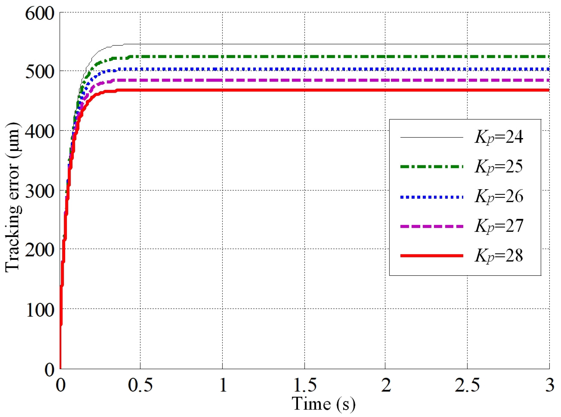
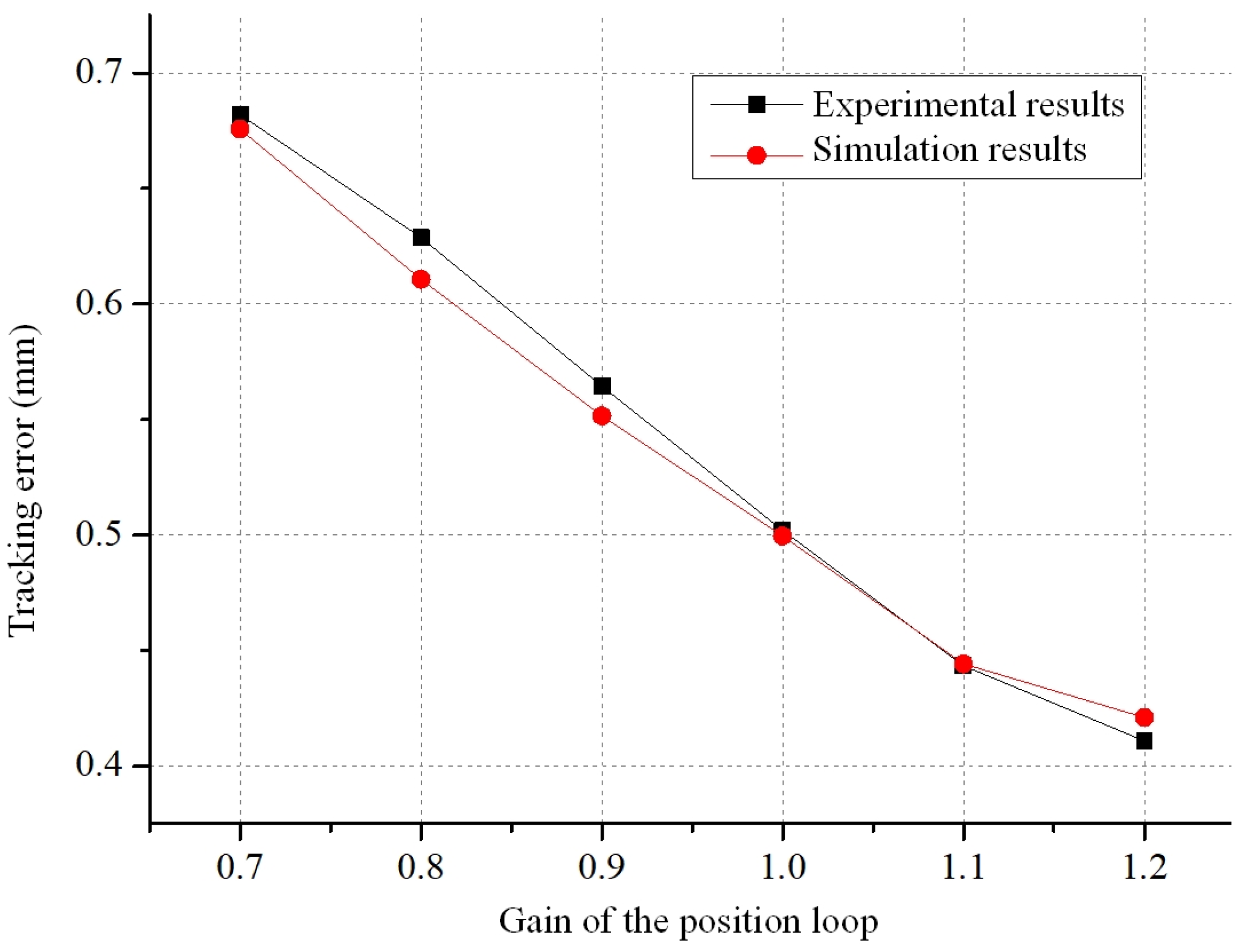
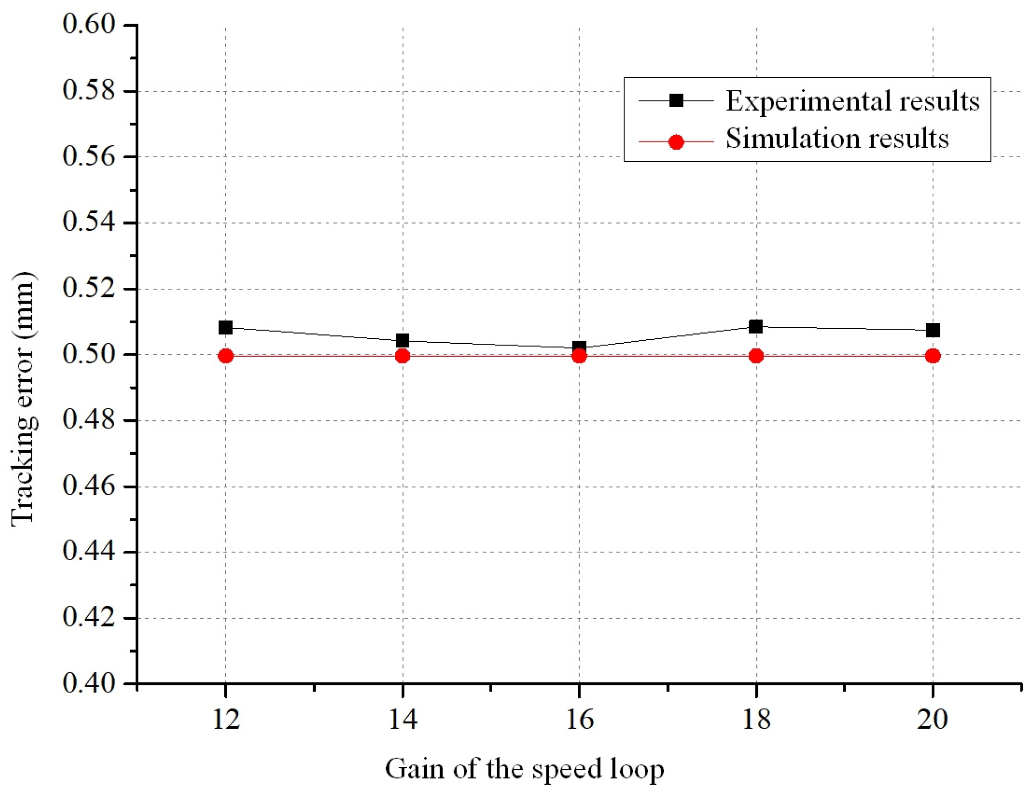
Effect of different gains on tracking error

With all other parameters held constant, simulation results for varying position gain (K_p) and velocity gain (K_s) are presented in Figure 23 and Figure 24, respectively.

From Figure 23, it can be observed that, as the position gain gradually increases, the tracking error also increases, and the tracking error is inversely correlated with the equivalent gain. However, the position loop gain cannot be increased indefinitely, as doing so might lead to system divergence and an increase in tracking error.

From Figure 24, it can be observed that changing the velocity loop gain has a minimal impact on the average value of the tracking error, but it does affect the stability of the tracking error curve. A higher velocity loop gain leads to greater fluctuations in the tracking error curve, consequently causing more significant oscillations in the tool tip trajectory. Therefore, it is essential to set the value of K_s appropriately.

4. Experimental Verification of the Servo Feed System Model for Heavy Vertical Machining Centres

This section focuses on the design of the experiments to verify the model of the servo feed system. First, the three-loop Bode plots of the CNC system and theoretical servo drive model are compared to validate the servo drive model. Then, to validate the mechanical transmission model, the measured critical stick-slip velocities of the X and Y axes are compared with the simulation results of the theoretical model.

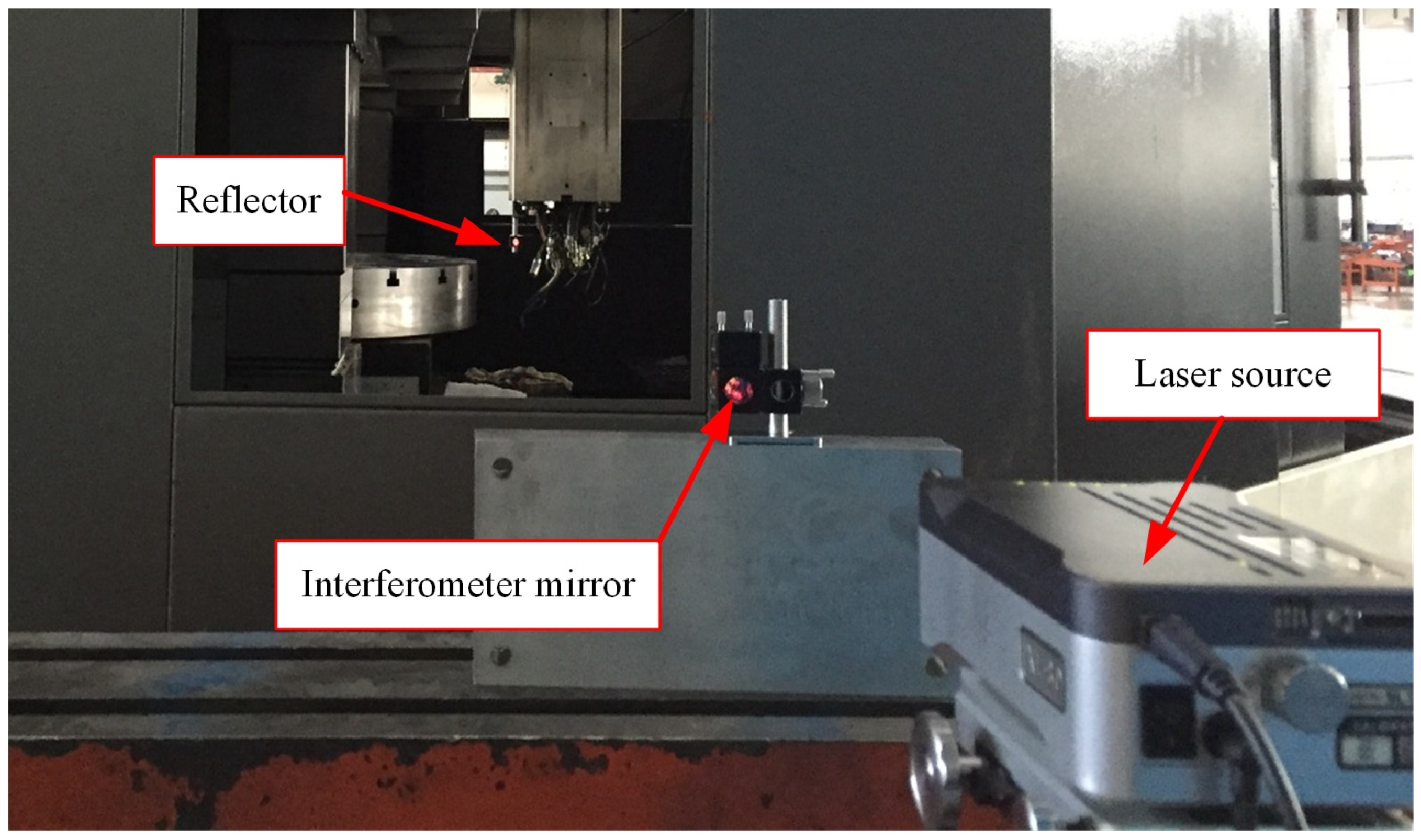
4.1. Experimental Setup

The Renishaw XL80 laser interferometer has been used for the motion measurements in the experiments. The LaserXL is used for data acquisition. Its main functions include the real-time collection and analysis of dynamic data from the Renishaw XL80 laser interferometer. A separate panel makes all key laser and environmental data visible. DyconXL can be used for the conversion of the *.RTX files into *.CRV files, allowing the collected data to be easily imported into applications such as MathCAD, Mathematica, and Excel for further analysis. Additionally, FFT vibration spectrum analysis can also be performed in the LaserXL software (Version 20.1), enabling accurate measurement of the dynamic characteristics of machine tools, coordinate measuring machines, and other motion systems.

In this experiment, it is necessary to measure the tracking error separately for the X and Y axes. Therefore, the measurement instruments are installed on both X and Y axes. The setup of the X-axis laser interferometer is shown in Figure 25.

After the experimental setup is completed, a set of experiments will be conducted according to the experiments plan. Single shot trigger mode is selected for the data capture in LaserXL, which means that data capture commences as soon as the X/Y axis starts to move.

4.2. Experimental Verification of the Theoretical Model of the Servo Feed System

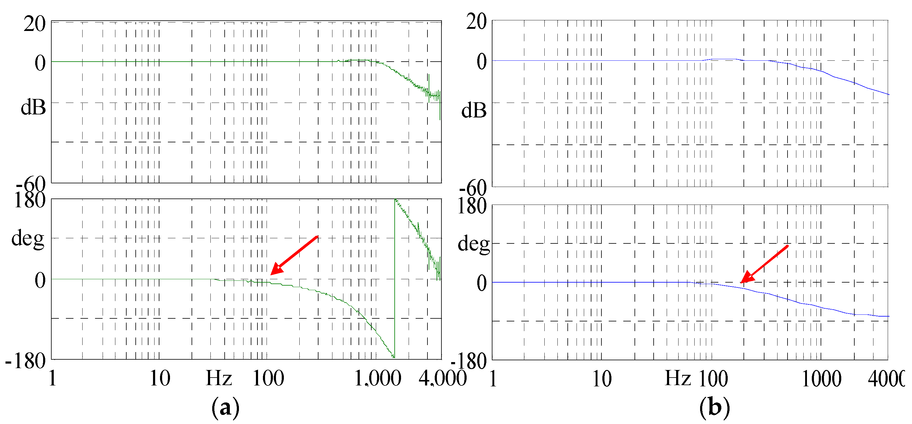
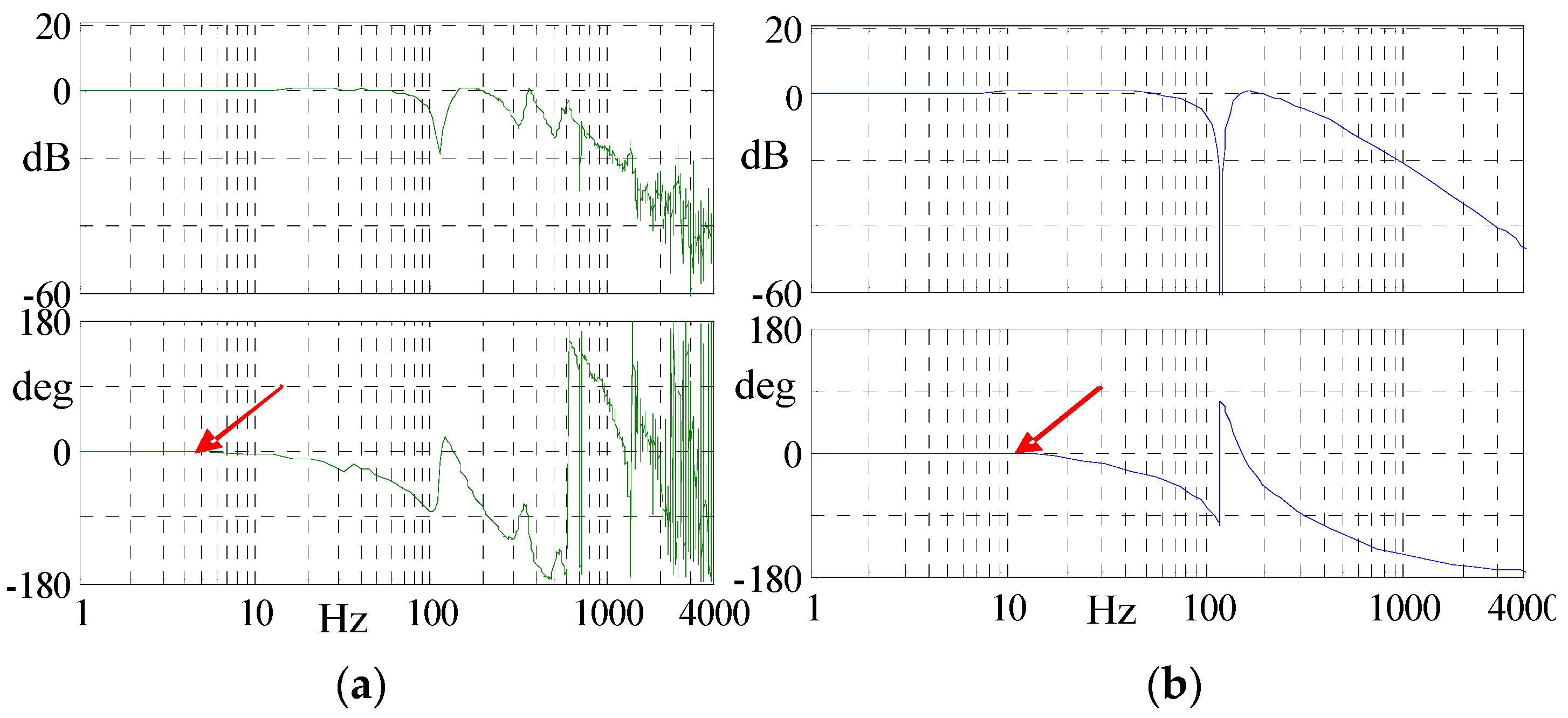
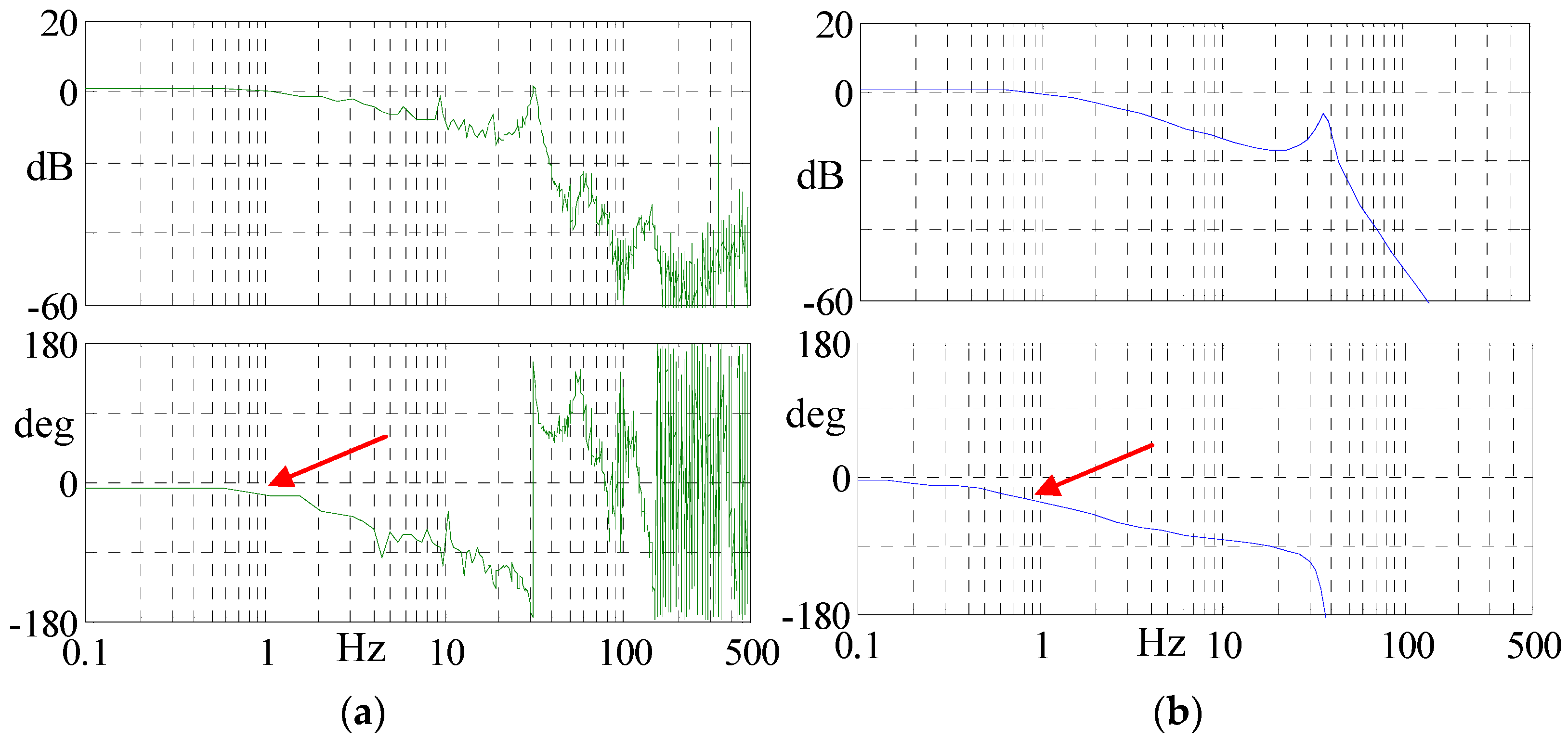
4.2.1. Verification of the Theoretical Model of the Servo Drive System

Startup Tools (Version 7.6) is a supporting software provided by Siemens for its CNC systems, which is used to optimize control systems. With this software, it is easy to read the characteristic curves inside the CNC system. For the machine tool used for this research, the Bode diagram of the current loop, velocity loop, and position loop can be obtained with pre-set parameters. Also, the Bode plots of the servo drive system can be achieved based on the developed theoretical model. The comparisons of the data obtained from Startup Tools and the theoretical model are demonstrated in Figure 26, Figure 27 and Figure 28.

From Figure 26, it can be seen that, within the frequency range of 1–1000 Hz, the amplitude response of the current loop for the actual CNC system and the servo drive model are all equal to 0. The phase response gradually changes from 0 to a negative value at around 100 Hz, indicated by the red arrow. This indicates that the current loop structure and the parameter settings of the theoretical model are consistent with those of the actual CNC system.

From Figure 27, it can be seen that, within the frequency range of 1–100 Hz, the amplitude response of the velocity loop for the actual CNC system and the servo drive model are all equal to 0. The phase response gradually changes from 0 to a negative value around 10 Hz, indicated by the red arrow. This indicates that the velocity loop structure and the parameter settings of the theoretical model are similar to those of the actual CNC system.

From Figure 28, it can be seen that, within the frequency range of 0.1–1 Hz, the amplitude response of the position loop for the actual CNC system and the servo drive model are all slightly greater than 0. The phase response gradually changes from 0 to a negative value around 1 Hz, indicated by the red arrow. This indicates that the position loop structure and the parameter settings of the theoretical model are close to those of the actual CNC system.

In summary, from the perspective of the Bode plots of the three-loop control, it can be concluded that the servo drive system model constructed in this study is essentially consistent with the actual one. This can serve as a foundation for subsequent research.

4.2.2. Verification of Critical Stick-Slip Velocity

In heavy-duty machine tools, the stick-slip phenomenon refers to the cyclic motion observed in the movement of machine tool components, characterized by intermittent alternations between rapid and slow motion. The stick-slip phenomenon is related to factors such as frictional resistance and system stiffness. Different types of machine tools have different limitations to stick-slip fluctuations.

Given the current lack of a well-defined quantity for stick-slip in the academic context, this paper proposes a specific criterion for defining stick-slip in the scope of this research, based on practical experiences: if the single stick-slip quantity of the machine tool reaches or surpasses 1 μm, it signifies the presence of the stick-slip phenomenon.

In the theoretical model of the servo feed system, the friction model is a combination of static friction, viscous friction, and Coulomb friction. Therefore, with abrupt changes in friction force caused by stick-slip, the critical stick-slip velocity of the X and Y axes can also be calculated. Since the modelling for both the X and Y axes is the same, the experimental results should be similar. Therefore, only the X-axis will be used as an example for illustration.

The machine tool carriage (X-axis) is driven at feed rates of 0.1 mm/min, 0.5 mm/min, 1 mm/min, 3 mm/min, 4 mm/min, and 5 mm/min to travel a certain distance. The time-displacement curves are recorded, as depicted in Figure 29. From the graph, it is noticeable that the critical stick-slip velocity for the X-axis falls within the range of 4 mm/min to 5 mm/min.

The theoretical model of the servo feed system is run in Simulink with different feed rates, i.e., 3 mm/min, 4 mm/min, and 5 mm/min. Simulated time-displaced curves are shown in Figure 30. It can be observed that the calculated critical stick-slip velocity also falls within the range of 4 mm/min to 5 mm/min. This indicates that the empirically measured critical stick-slip velocity and the simulated critical stick-slip velocity align within the same velocity interval.

In summary, it can be seen that the critical stick-slip velocity of the heavy-duty vertical machining centre under investigation maintains consistency across both simulation and experimental findings, which indicates the accuracy of the developed friction model and, by extension, indirectly validates the accuracy of the theoretical model of mechanical transmission.

4.2.3. Tracking Error for Linear Motion of X-Axis

Since the same modelling method has been applied to both the X-axis and the Y-axis, the motion error variation will be similar for the two axes. Therefore, single-axis experiments are carried out, taking the X-axis as an example to illustrate. The actual measured error and the theoretical simulated error for the X-axis linear motion trajectory are presented in

Table 3. Tracking error of the X-axis at different feed rates.

Feed Rate (mm/min)	Measured Tracking Error (mm)	Simulated Tracking Error (mm)
100	0.0976	0.09993
200	0.1792	0.19986
300	0.3015	0.29979
400	0.3725	0.39972
500	0.502	0.49965
600	0.6011	0.59958
700	0.6977	0.69951
800	0.7926	0.79944
900	0.9108	0.89937
1000	1.0104	0.99936

, and the corresponding plots of feed rate vs. tracking error are given in Figure 31.

From the results shown in Figure 31, it can be seen that the trend of the actual tracking error and simulated tracking error of the X-axis is the same, both increasing with the increase of the feed rate. Furthermore, the tracking error of the simulation is consistent with the measured actual results.

It can be derived theoretically that the tracking error of the straight-line trajectory increases with the increase of equivalent gain, while the equivalent gain of the closed-loop system is related to both the position loop gain and the velocity loop gain. Therefore, it is considered to measure and record the tracking error during linear motion for different position loop gains and velocity loop gains of the servo system with a fix feed rate of 500 mm/min. The measured actual error and theoretical simulation error of the X-axis linear motion trajectory are shown in

Table 4. Tracking error of the X-axis with different position loop gains.

Kp (m/min/mm)	Measured Tracking Error (mm)	Simulated Tracking Error (mm)
0.7	0.6820	0.6757
0.8	0.6288	0.6107
0.9	0.5645	0.5516
1	0.5020	0.4996
1.1	0.4434	0.4442
1.2	0.4109	0.4210

, and the corresponding plots of position loop gain vs. tracking error are given in Figure 32.

From the data in Table 4 and Figure 32, it can be seen that the larger the position loop gain K_p, the smaller the tracking error. Moreover, the simulated tracking errors from the theoretical model are similar to the actual measurement outcomes.

The measured actual tracking error and the theoretical simulation error of the linear motion trajectory of the X-axis, with different velocity loop gains K_s, are shown in

Table 5. Tracking error for different velocity loop gains of the X-axis.

Ks (N·m·s/rad)	Measured Tracking Error (mm)	Simulated Tracking Error (mm)
12	0.5083	0.49965
14	0.5042	0.49965
16	0.502	0.49965
18	0.5085	0.49965
20	0.5075	0.49965

. The corresponding plots of velocity loop gain vs. tracking error are given in Figure 33.

From the data in Table 5 and Figure 33, it can be seen that the calculated tracking errors are close to the actual measurement results.

Based on the comparison of the actual measurement error and theoretical simulation error of the linear motion trajectory for a single axis, it can be seen that the tracking errors of the theoretical model simulation are similar to the actual measurement results for different feed rates, position loop gains. and velocity loop gains. It can be concluded that the developed theoretical model of the servo feed system is correct, and tracking errors can be predicted for a single axis.

5. Conclusions

In this paper, a theoretical model for the servo feed system of a heavy-duty vertical machining centre was developed. The model considered its characteristics of large mass, significant load, and large travel. The servo feed system model includes friction, backlash, and lateral shift models. Additionally, a Simulink simulation model for the servo feed system was established, and the main influencing factors and their influencing laws of motion tracking error were analysed through simulation. This paper also includes theoretical model validation experiments, with simulation results compared to experimental results. The main conclusions of this paper are as follows:

(1)

A theoretical model of the servo feed system for heavy-duty vertical machining centres was created. The model takes into account the characteristics of large mass, large load, and large travel distance, and consists of the servo drive system model and the mechanical transmission system model. The servo drive system model adopts a three-loop control structure commonly used in commercial CNC systems, such as Siemens, FANUC, HEIDENHAIN. The mechanical transmission system model encompasses non-linear aspects such as friction, backlash, and lateral shifts.

(2)

The Simulink simulation model for the theoretical servo feed system was established and, through simulations, it was determined that larger backlash, greater offset of the tool holder from the beam centre, and higher feed rates lead to larger tracking errors. Moreover, there exists a positive correlation between tracking error and feed rate. Larger position loop gains result in smaller tracking errors. The impact of the viscous friction coefficient and the velocity loop gain on the tracking error is minimal and can be ignored. On the other hand, the static-to-dynamic friction ratio and the Coulomb friction coefficient primarily affect tracking errors during machine tool startup.

(3)

Experiments have been carried out to validate the developed theoretical models. The comparison of Bode plots between the actual CNC drive system and the theoretical models of the servo drive system, both employing a three-loop structure, indicates the validity of the drive system’s theoretical model. The agreement between the measured critical stick-slip velocity range for the X-axis, and the velocity range obtained from the theoretical model simulation, validates the accuracy of the model of the mechanical transmission system. Through a comparison of measured tracking error and theoretical simulation outcomes for the X-axis in linear motion, the accuracy of the developed servo feed system model is confirmed and the feasibility of analysing dynamic servo errors in real machine tools is demonstrated.

References

1. Uriarte, L.; Zatarain, M.; Axinte, D.; Yagüe-Fabra, J.; Ihlenfeldt, S.; Eguia, J.; Olarra, A. Machine tools for large parts. CIRP Ann.-Manuf. Technol. 2013, 62, 731–750. [Google Scholar] [CrossRef]
2. Andolfatto, L.; Lavernhe, S.; Mayer, J.R.R. Evaluation of servo, geometric and dynamic error sources on five-axis high-speed machine tool. Int. J. Mach. Tools Manuf. 2011, 51, 787–796. [Google Scholar] [CrossRef]
3. Bringmann, B.; Maglie, P. A method for direct evaluation of the dynamic 3D path accuracy of NC machine tools. CIRP Ann.-Manuf. Technol. 2009, 58, 343–346. [Google Scholar] [CrossRef]
4. Jia, Z.; Ma, J.; Song, D.; Wang, F.; Liu, W. A review of contouring-error reduction method in multi-axis CNC machining. Int. J. Mach. Tools Manuf. 2018, 125, 34–54. [Google Scholar] [CrossRef]
5. Lyu, D.; Liu, Q.; Liu, H.; Zhao, W. Dynamic error of CNC machine tools: A state-of-the-art review. Int. J. Adv. Manuf. Technol. 2020, 106, 1869–1891. [Google Scholar] [CrossRef]
6. Lin, C.-Y.; Luh, Y.-P.; Lin, W.-Z.; Lin, B.-C.; Hung, J.-P. Modeling the static and dynamic behaviors of a large heavy-duty lathe machine under rated loads. Computation 2022, 10, 207. [Google Scholar] [CrossRef]
7. Poo, A.N.; Bollinger, J.G.; Younkin, G.W. Dynamic errors in type-I contouring systems. IEEE Trans. Ind. Appl. 1972, 4, 477–484. [Google Scholar] [CrossRef]
8. Xi, X.C.; Poo, A.N.; Hong, G.S. Improving contouring gain accuracy by tuning gain for a bi-axial CNC machine. Int. J. Mach. Tools Manuf. 2009, 49, 395–406. [Google Scholar] [CrossRef]
9. Koren, Y. Cross-coupled biaxial computer control for manufacturing systems. ASME J. Dyn. Syst. Meas. Control 1980, 102, 265–272. [Google Scholar] [CrossRef]
10. Koren, Y.; Lo, C.C. Variable-gain cross-coupling controller for contouring. CIRP Ann.-Manuf. Technol. 1991, 40, 371–374. [Google Scholar] [CrossRef]
11. Yeh, S.S.; Hsu, P.L. Estimation of the contouring error vector for the cross-coupled control design. IEEE/ASME Trans. Mechatron. 2022, 7, 44–51. [Google Scholar]
12. Peng, C.C.; Chen, C.L. Biaxial contouring control with friction dynamics using a contour index approach. Int. J. Mach. Tools Manuf. 2007, 47, 1542–1555. [Google Scholar] [CrossRef]
13. Cheng, M.Y.; Lee, C.C. Motion controller design for contour following tasks based on real-time contour error estimation. IEEE Trans. Ind. Electron. 2007, 54, 1686–1695. [Google Scholar] [CrossRef]
14. Yang, J.; Li, Z. A novel contour error estimation for position loop-based cross-coupled control. IEEE Trans. Mechatron. 2011, 16, 643–655. [Google Scholar] [CrossRef]
15. Huo, F.; Xi, X.C.; Poo, A.N. Generalized Taylor series expansion for free-form two-dimensional contour error compensation. Int. J. Mach. Tools Manuf. 2012, 53, 91–99. [Google Scholar] [CrossRef]
16. Conway, J.R.; Ernesto, C.A.; Farouki, R.T.; Zhang, M. Performance analysis of cross-coupled controllers for CNC machines based upon precise real-time contour error measurement. Int. J. Mach. Tools Manuf. 2012, 52, 30–39. [Google Scholar] [CrossRef]
17. Yu, H.; Zhang, L.; Wang, C.; Feng, X. Dynamic characteristics analysis and experimental of differential dual drive servo feed system. Proc. Inst. Mech. Eng. Part C J. Mech. Eng. Sci. 2021, 235, 6737–6751. [Google Scholar] [CrossRef]
18. Shi, S.; Lin, J.; Wang, X.; Xu, X. Analysis of the transient backlash error in CNC machine tools with closed loops. Int. J. Mach. Tools Manuf. 2015, 93, 49–60. [Google Scholar] [CrossRef]
19. Wan, M.; Dai, J.; Zhang, W.H.; Xiao, Q.B.; Qin, X.B. Adaptive feed-forward friction compensation through developing an asymmetrical dynamic friction model. Mech. Mach. Theory 2022, 170, 104691. [Google Scholar] [CrossRef]
20. Yamada, S.; Fujimoto, H. Precise joint torque control method for two-inertia system with backlash using load-side encoder. IEEJ J. Ind. Appl. 2019, 8, 75–83. [Google Scholar] [CrossRef]
21. Wang, Z.; Hu, C.; Zhu, Y. Double Taylor expansion-based real-time contouring error estimation for multi-axis motion systems. IEEE Trans. Ind. Electron. 2019, 66, 9490–9499. [Google Scholar] [CrossRef]
22. Kim, S. Moment of inertia and friction torque coefficient identification in a servo drive system. IEEE Trans. Ind. Electron. 2018, 66, 60–70. [Google Scholar] [CrossRef]
23. Ebrahimi, M.; Whalley, R. Analysis, modeling and simulation of stiffness in machine tool drives. Comput. Ind. Eng. 2000, 38, 93–105. [Google Scholar] [CrossRef]
24. Otten, G.; de Vries, T.J.A. Linear motor motion control using a learning feed forward controller. IEEE/ASME Trans. Mechatron. 1997, 2, 179–187. [Google Scholar] [CrossRef]
25. Shiau, T.N.; Huang, K.H.; Hsu, W.C. Dynamic response and stability of a rotating ball screw under a moving skew load. J. Chin. Soc. Mech. Eng. Ser. C 2006, 27, 297–305. [Google Scholar]
Figure 1. A heavy-duty vertical machining centre. (a) Machine tool configuration. (b) Picture of the machine tool.
Processes 11 02930 g001
Figure 2. Block diagram of the three-loop control structure.
Processes 11 02930 g002
Figure 3. Structural diagram of a Siemens control system [23].
Processes 11 02930 g003
Figure 4. Current loop control structure diagram.
Processes 11 02930 g004
Figure 5. Velocity loop control structure diagram.
Processes 11 02930 g005
Figure 6. Position loop control structure diagram with feedforward function.
Processes 11 02930 g006
Figure 7. Structure of a ball screw servo feed system.
Processes 11 02930 g007
Figure 8. Equivalent diagram of the mechanical components of the ball screw feed system.
Processes 11 02930 g008
Figure 9. Block diagram of the mechanical transmission system.
Processes 11 02930 g009
Figure 10. Classification of static friction models.
Processes 11 02930 g010
Figure 11. Schematic diagram of a mechanism with backlash.
Processes 11 02930 g011
Figure 12. Schematic diagram of beam with the force and deformation.
Processes 11 02930 g012
Figure 13. Complete block diagram of the mechanical transmission.
Processes 11 02930 g013
Figure 14. The decomposition of the position command for linear motion trajectory. (a) Position command of a linear motion trajectory. (b) Decomposed position command of X and Y axes.
Processes 11 02930 g014
Figure 15. Input for linear trajectory in Simulink.
Processes 11 02930 g015
Figure 16. Single-axis closed-loop servo feed system.
Processes 11 02930 g016
Figure 17. Time vs. tracking error curves for different static-to-dynamic friction ratios.
Processes 11 02930 g017
Figure 18. Time vs. tracking error curves for different coulomb friction coefficients.
Processes 11 02930 g018
Figure 19. Time vs. tracking error curves for different viscous friction coefficients.
Processes 11 02930 g019
Figure 20. Error curves of circular trajectory for different backlashes.
Processes 11 02930 g020
Figure 21. Error curves of linear trajectory tool holder at different positions.
Processes 11 02930 g021
Figure 22. Time vs. tracking error curves for different feed rates.
Processes 11 02930 g022
Figure 23. Time vs. tracking error curves for different position gains.
Processes 11 02930 g023
Figure 24. Time vs. tracking error curves for different velocity loop gains.
Processes 11 02930 g024
Figure 25. Setup of X-axis laser interferometer.
Processes 11 02930 g025
Figure 26. Comparison of Bode plots of current loops. (a) Bode plot of current loop for actual CNC system. (b) Bode plot of current loop for the servo drive system model.
Processes 11 02930 g026
Figure 27. Comparison of Bode plots of velocity loops. (a) Bode plot of velocity loop for actual CNC system. (b) Bode plot of velocity loop for the servo drive system model.
Processes 11 02930 g027
Figure 28. Comparison of Bode plots of position loops. (a) Bode plot of position loop for actual CNC system. (b) Bode plot of position loop for servo drive system model.
Processes 11 02930 g028
Figure 29. Measured time vs. displacement curves of the X-axis at different feed rates.
Processes 11 02930 g029
Figure 30. Simulated time vs. displacement curves for the X-axis at different feed rates.
Processes 11 02930 g030
Figure 31. Feed rate vs. tracking error curves for X-axis.
Processes 11 02930 g031
Figure 32. Position loop gain vs. tracking error curves for X-axis.
Processes 11 02930 g032
Figure 33. Velocity loop gain vs. tracking error curves for X-axis.
Processes 11 02930 g033