Experimental Simulation on the Stress Disturbance Mechanism Caused by Hydraulic Fracturing on the Mechanical Properties of Shale Formation

Abstract

Hydraulic fracturing is an indispensable technology for the development of shale oil and shale gas. Knowing the changes in the rock mechanical properties and failure modes during hydraulic fracturing is the key to improving the efficiency of hydraulic fracturing. Based on experiments and simulations, it can be concluded that the injection of fracturing fluid in the hydraulic fracturing caused deformation of the fracture surface, and the rock mechanical properties experienced degradation with a maximum reduction in the rock mechanical properties of 44.24%. As indicated in the experiments, the displacement of the measurement point was decreased with the distance increase between the injection point and the measurement point. According to the numerical simulations, tensile failure is the main failure mode in hydraulic fracturing, but the percentage of shear failure had an obvious increase with the increase in distance between the injection point and the measurement point. Comparing DDS #1 and DDS #5, the DDS #5 measurement point was farther away from the injection point, and the average percentage of shear failure increased from 21.94 to 52.72%. Meanwhile, the increase in the branch fractures also caused shear failure to occur. Comparing Sample 1 and Sample 3, in Sample 3, which had more branch fractures, the average percentage of shear failure increased from 33.12 to 37.58%. Due to the porous medium of the reservoir rock, the enormous pressure generated during the injection of fracturing fluid caused significant deformation of the fracture surface, leading to the tensile failure of the rock. The displacement of the fracture surface caused by the fracturing fluid injection also led to the deformation of the pore throat structure; thus, the shear failure increased when the measurement point was away from the injection point.

1. Introduction

With the increasing demand for oil and gas resources, shale gas and shale oil are playing an important role in guaranteeing the supply of oil and gas resources, and stimulated reservoir volume is an essential technology to improve shale oil and gas recovery [1,2,3]. In the process of hydraulic fracturing practice, relevant scholars have found that in the process of hydraulic fracture expansion, fracturing water permeates along both sides of the fracture, forming a pore pressure gradient, forming an additional disturbed stress field, and superimposing on the ground stress to form a new stress distribution, changing the original stress distribution state inside the reservoir [4,5,6]. Affected by hydraulic fracturing, the conductivity of the hydraulic fracture and the permeability of the shale rock experience significant changes because of the stress disturbance produced by hydraulic fracturing [7,8,9]. Clarifying the stress disturbance mechanism during hydraulic fracturing is of great significance for improving shale oil and gas recovery.

In shale reservoirs, horizontal wells are drilled along the minimum horizontal principal stress direction, which may cross natural fractures [10]. These fractures can have a significant impact on the trajectory and shape of the hydraulic fractures during the fracturing process [11,12]. Cheng et al. proposed an equation for the intersection of hydraulic and natural fractures in 3D space and verified it through indoor experiments. However, the stress difference they simulated and experimented with may not fully reflect the stress difference present in deep shale. Xu et al. proposed a new hydraulic fracture–natural fracture interaction model. They conducted a sensitivity analysis on the key influencing parameters, such as the stress difference and natural fracture direction. Ren et al. established a three-dimensional modified displacement discontinuity method (DDM) model and discussed the influence of the engineering parameters on the fracture morphology and reservoir modification area under the influence of natural fractures. However, the fracture model width was consistent in the longitudinal direction, and it was hard to fully reflect the fracture morphology. Zhu and Zheng et al. proposed a 3D hydraulic fracture model based on the finite element method to investigate the influence of the stress field on fracture propagation. The simulations indicated that the induced stress field was the main factor confining the fracture propagation, and increasing the fracture space and pumping rate promoted fracture propagation. To further understand the change in the stress field during the whole production period, the ABAQUS and Computer Modelling Group Ltd. (CMG) (Calgary, AB, Canada) simulator was introduced to analyze the induced stress and production change [13,14,15,16,17,18,19].

From the previous research, it can be concluded that the hydraulic fracture propagation mechanism in shale formation is understood, and the factors affecting fracture propagation have been analyzed. However, the displacement and stress disturbance caused by hydraulic fracturing have not been clarified, as reservoir rock is a porous medium, which was the main factor affecting the optimization of the fracture conductivity and production [20,21]. Since most shale reservoirs are several thousand meters underground, it is not realistic to study the mechanism of stress disturbance under different conditions in hydraulic fracturing field practice. However, most indoor hydraulic fracturing experiments are conducted by direct observation of the hydraulic fracture propagation morphology on the surface and inside test blocks by the naked eye and high-speed photography [22,23,24]. However, this method makes it difficult to study the distribution of the stress field inside the test block and the layer microfracture zone caused by stress disturbance in the process of hydraulic fracturing [25,26,27,28,29]. Based on the true triaxial hydraulic fracturing test, combined with distributed displacement sensors (DDSs) to monitor the displacement changes, and supplemented by CT to observe the changes in the rock micropore structure, we can simultaneously observe the distribution of microfractures and stress changes in the test block. On this basis, a numerical simulation model was established to understand the stress disturbance mechanism and rock mechanical property distribution during hydraulic fracturing, which is of great significance to increasing the volume of shale reservoir production.

2. Experimental Simulation

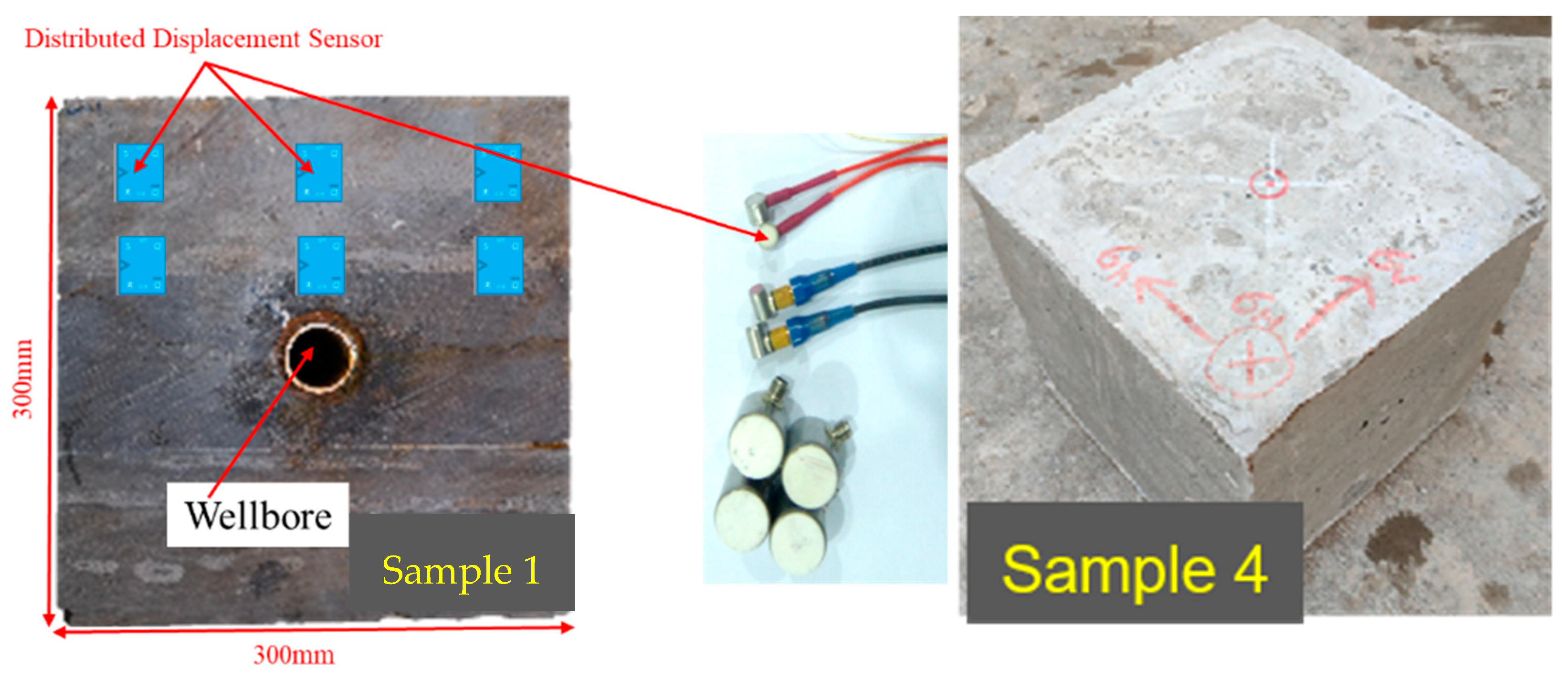
2.1. Experimental Devices

As indicated in Figure 1, using a true triaxial large-scale hydraulic fracturing simulation system, horizontal well multi-segment cluster fracturing simulation experiments were conducted on large-sized outcrop mudstone/shale thin interlayered samples. The true triaxial pressure loading system achieved a maximum stress of 30 MPa in the vertical (Z-axis) and horizontal (Y-axis) directions when subjected to confining pressure loading on the specimen; the maximum stress in the horizontal direction (X-axis) reached 15 MPa. The loading process adopted a variable frequency loading technology, which was quickly pressurized through a hydraulic station and then precisely pressurized through a control panel, enabling servo tracking of the pressure. The constant speed and pressure pump adopted a dual-cylinder continuous liquid supply method, with a maximum displacement of 300 mL/min.

2.2. Experimental Method and Schedule

To understand the change in the rock mechanical properties caused by hydraulic fracturing, four shale samples with a size of 300 mm × 300 mm × 300 mm were used in a true triaxial hydraulic fracturing experiment. In the experiment, the distributed displacement sensors (DDSs) were applied to monitor the displacement change in the shale rock during hydraulic fracturing [30]. As indicated in Figure 1, the row spacing between two sensors was 100 mm, and the column spacing between two sensors was 70 mm. The rock mechanical properties and injection parameters of the experiments are shown in

Table 1. The experimental parameters of the true triaxial hydraulic fracturing experiment.

Item	Parameters	Sample 1	Sample 2	Sample 3	Sample 4
Stress Field	Vertical stress/MPa	18.0	18.0	18.0	18.0
	Maximum horizontal principal stress/MPa	13.0	15.0	13.0	13.0
	Minimum horizontal principal stress/MPa	11.0	11.0	11.0	11.0
Rock Mechanical Properties	Young’s Modulus/GPa	34.2	34.2	34.2	34.2
	Poisson’s Rate	0.264	0.264	0.264	0.264
Injection Parameters	Injection rate/(mL/min)	5.0	5.0	8.0	5.0
	Viscosity of fracturing fluid/(mPa·s)	1.0	1.0	1.0	25.0

. In the experiments, the influence of the stress field, the injection rate, and the viscosity of the fracturing fluid on the fracture propagation were analyzed based on the true triaxial hydraulic fracturing test, combined with the distributed displacement sensors (DDSs) to monitor the displacement changes, and supplemented by CT to observe the changes in the rock micropore structure.

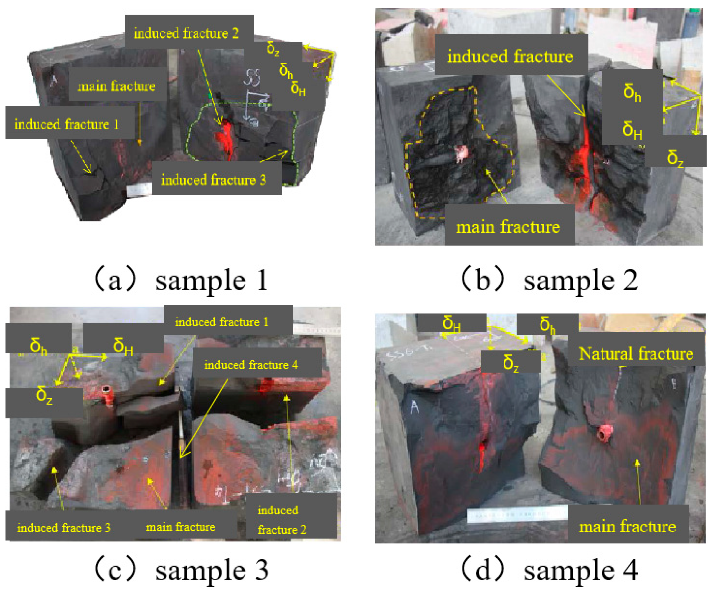
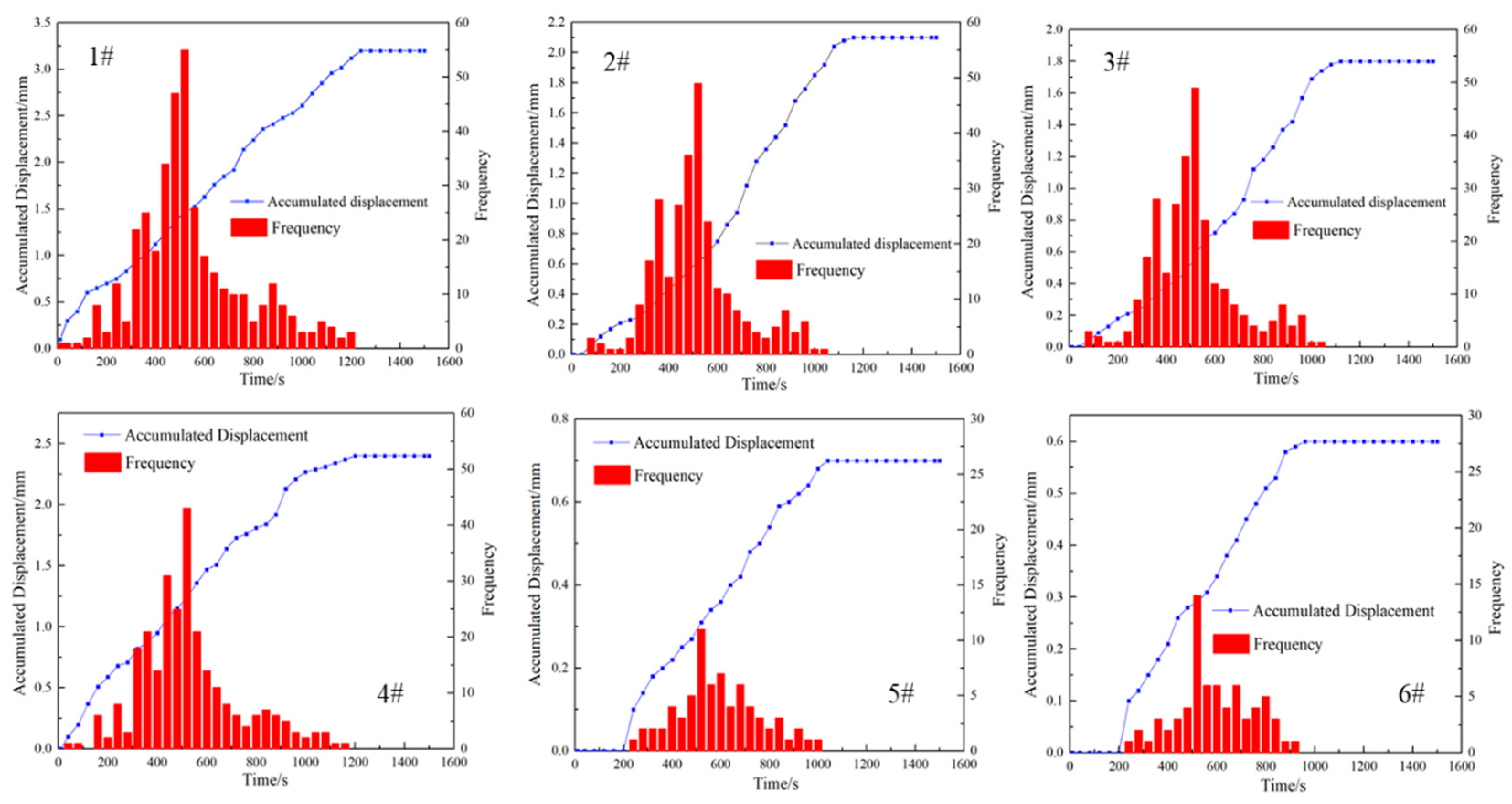
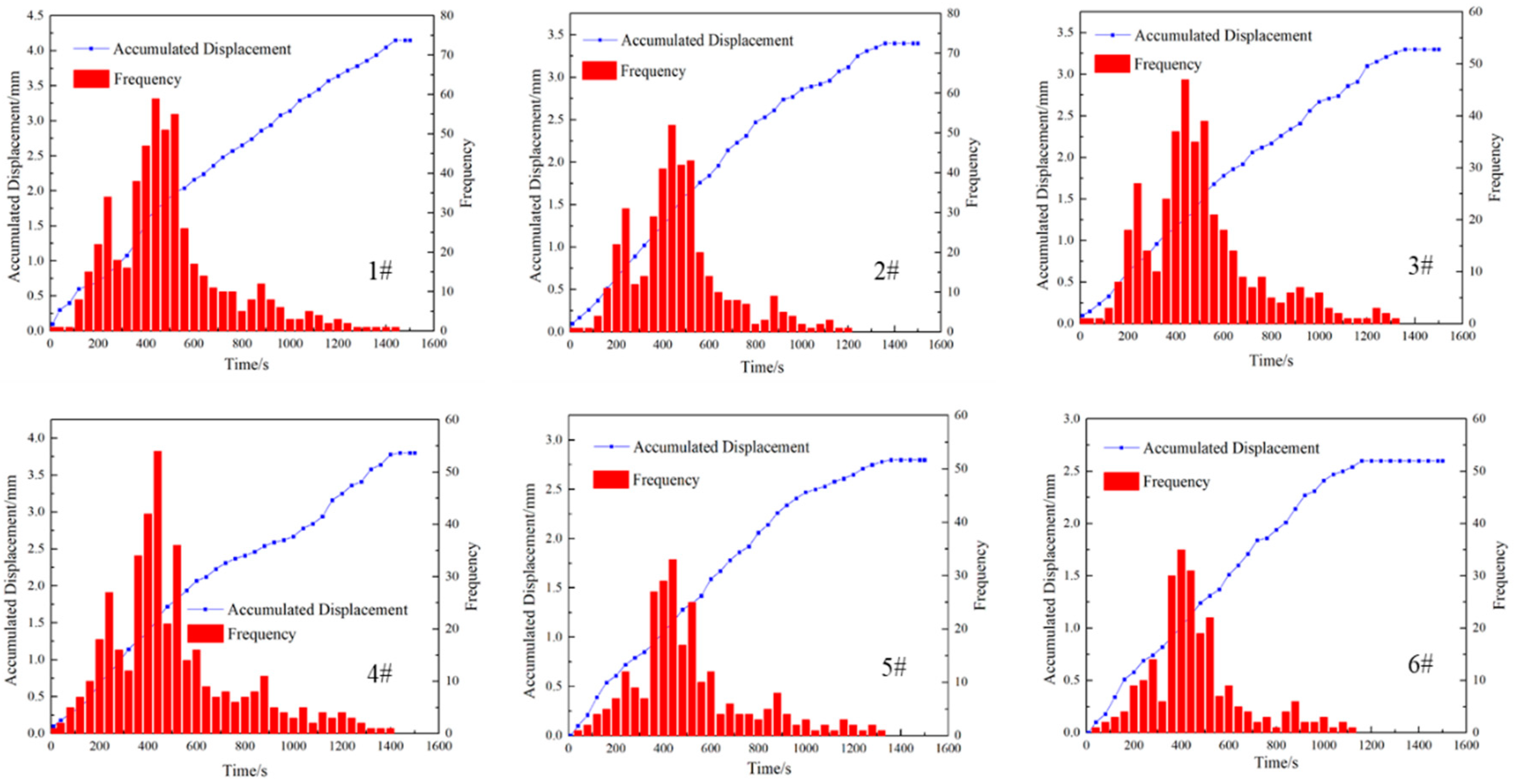
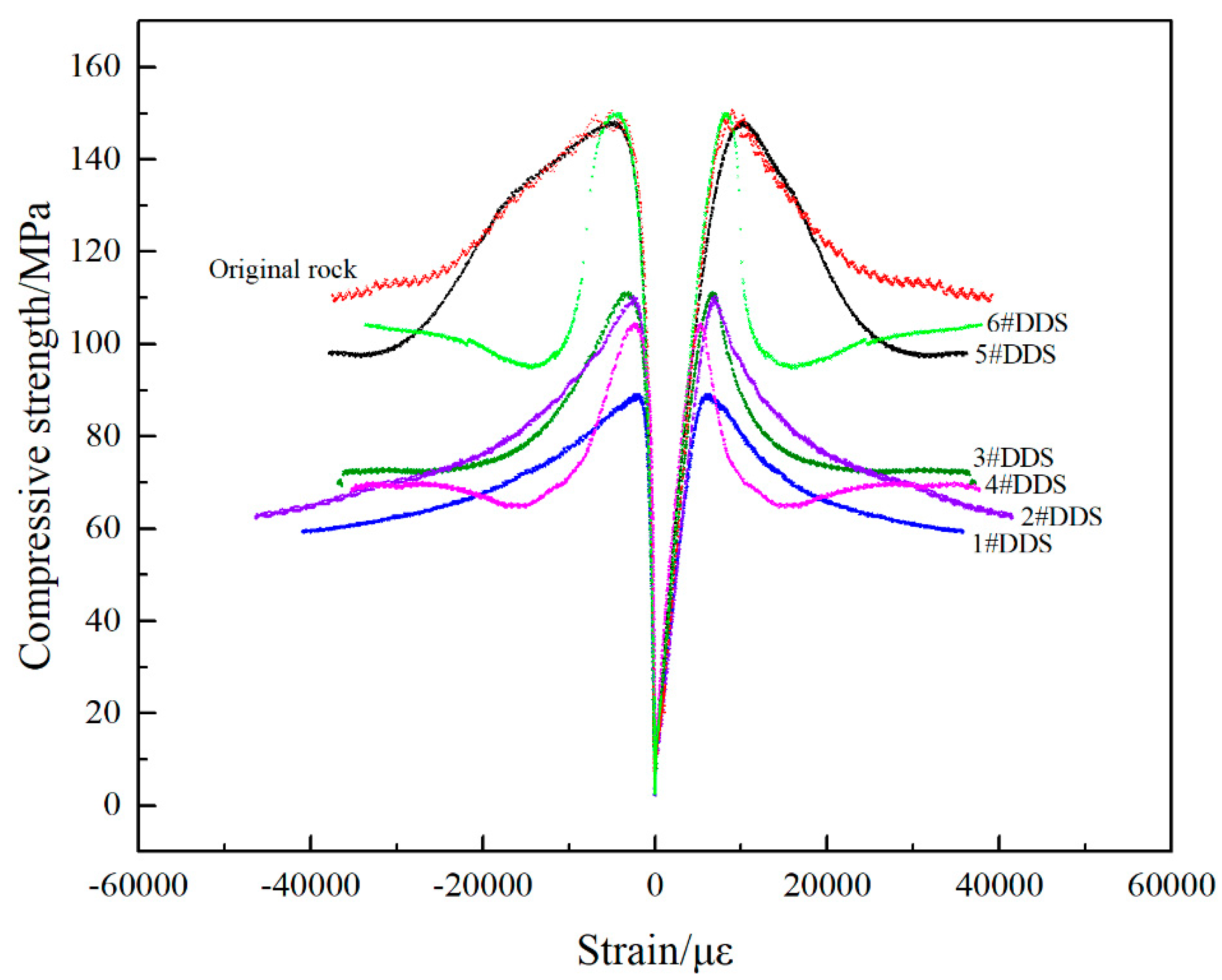
2.3. Experimental Results

Figure 2a–d and Figure 3a–d show the fracture geometries of Sample 1–Sample 4. As indicated in Sample 1 (Figure 2a and Figure 3a), Sample 2 (Figure 2b and Figure 3b), Sample 3 (Figure 2c and Figure 3c), and Sample 4 (Figure 2d and Figure 3d), it can be found that main fractures were created in the center of the samples, while the number of induced fractures had significant changes. When the horizontal principal stress difference was 2.0 MPa, three induced fractures were created, while only one induced fracture was created when the horizontal principal stress difference increased to 4.0 MPa (Figure 2b and Figure 3b). A high pumping rate also contributed to the formation of induced fractures. When the pumping rate increased to 8.0 mL/min, it was found that four induced fractures were created compared to Sample 1. Meanwhile, increasing the viscosity of the fracturing fluid was averse to creating a branch fracture. When the viscosity of the fracturing fluid increased from 1.0 mPa·s to 25.0 mPa·s, only one main fracture was created.

To further analyze the change in the displacement and signal frequency, the data obtained from the DDSs were analyzed. Figure 4 shows the changes in the accumulated displacement and signal frequency with the injection time. As indicated by DDS #1, the displacement of Sample 1 was 3.24 mm, the total signal frequency was 381, the peak frequency was obtained when the time was 520 s, and the peak frequency, which was obtained from DDS #1, was 55. The displacement of DDSs #2 and #3 decreased to 2.06 mm and 2.17 mm, and the total signal frequencies were 276 and 283, respectively. For DDSs #2 and #3, the peak frequencies were 47 and 49, which were obtained at 534 s. For DDS #4, the displacement and total frequency were 2.45 mm and 306, and the peak frequency was 53 when the time was 527 s. Due to the signal strength being further weakened, the displacements of DDSs #5 and #6 were 0.63 mm and 0.71 mm, respectively, the total frequencies were 68 and 71, and the peak frequencies were 11 and 14, which were obtained when the time was 538 s. From the experimental data, the displacement signals were distributed between 0 and 1240 s for DDS #1, and no signal was detected when the time exceeded 1240 s. For DDSs #2, #3, and #4, the displacement signals were distributed between 0 and 1160 s, while the displacement signals were only distributed between 0 and 960 s.

Figure 5 shows the changes in the accumulated displacement and signal frequency with injection time in Sample 2. In this experiment, the horizontal principal stress difference increased to 4.0 MPa. As shown in Figure 5, it was found that the displacement of DDS #1 was 2.91 mm, the peak frequency was 38 when the injection time was 580 s, and the total frequency was 358. For DDSs #2 and #3, the displacement experienced dramatic decreases in the displacement to 1.53 mm and 1.48 mm, and the total frequencies were 232 and 217, respectively. It should be noted that the peak frequencies of DDSs #2 and #3 were 27 and 24 when the injection time was 585 s, and the corresponding displacements were 0.57 mm and 0.54 mm, respectively. For DDS #4, the displacement and total frequency were 2.34 mm and 263, and the maximum peak frequency was 29 when the injection time was 582 s. The displacements of DDSs #5 and #6 were 0.43 mm and 0.41 mm, and the total frequencies were 43 and 40, respectively. In addition, the peak frequencies of DDSs #5 and #6 were 8 and 7 when the injection time was 592 s, and the corresponding displacements were 0.28 mm and 0.31 mm. As indicated in Figure 5, it can be found that the displacement signals of DDSs #1, #2, #3, and #4 were distributed from 0 to 1400 s. When the time exceeded 880 s, DDSs #5 and #6 could not detect the displacement signal.

When the pumping rate increased to 8.0 m³/min, the signals of the DDSs experienced significant changes. As shown in Figure 6, the accumulated displacement and total signal frequency were 4.15 mm and 524 for DDS #1, the peak frequency appeared at 443 s with 59, and the corresponding displacement was 1.74. For DDSs #2 and #3, the accumulated displacements decreased to 3.41 mm and 3.35 mm, and the total signal frequencies decreased to 404 and 392, respectively. When the injection time was 452 s, the peak frequency was obtained with peak values at 47 and 46, and the corresponding displacements were 1.37 mm and 1.35 mm. For DDS #4, the accumulated displacement and total signal frequency were 3.78 mm and 414, and the peak frequency was 52 with a corresponding displacement of 1.72 mm when the injection time was 449 s. The accumulated displacement for the other two DDSs were 2.73 mm and 2.81 mm, with total signal frequencies of 238 and 245 and peak frequencies of 31 and 33, with corresponding displacements of 1.24 mm and 1.28 mm.

When the viscosity of the fracturing fluid increased from 1.0 mPa·s to 25.0 mPa·s, the displacement signal experienced significant changes. As indicated in Figure 7, it was found that the total displacement of DDS #1 was 3.42 mm, and the accumulated frequency was 384. From the detailed data of DDS #1, the peak frequency was 54, which was obtained at the injection time of 362 s, and the corresponding displacement was 0.83 mm. For DDSs #2 and #3, the total displacements decreased to 1.24 mm and 1.31 mm, and the accumulated frequencies decreased to 111 and 104, respectively. Meanwhile, the peak frequencies of DDSs #2 and #3 were 22 and 19 when the injection time was 368 s, respectively, and the corresponding displacements were 0.76 mm and 0.74 mm. As for DDS #4, the total displacement and accumulated frequency were 1.36 mm and 127, the peak frequency was 27, which was obtained when the injection time was 364 s, and the corresponding displacement was 0.79 mm. Due to the signal strength being further weakened, the displacements of DDSs #5 and #6 were 0.44 mm and 0.42 mm, the total frequencies were 41 and 37, and the peak frequencies were 10 and 8, obtained when the time was 371 s. In Figure 7, it also can be seen that the displacement signal of DDS #1 was distributed from 0 to 1420 s, while the other five DDSs could not detect the signals when the injection time exceeded 600 s.

3. Discussion

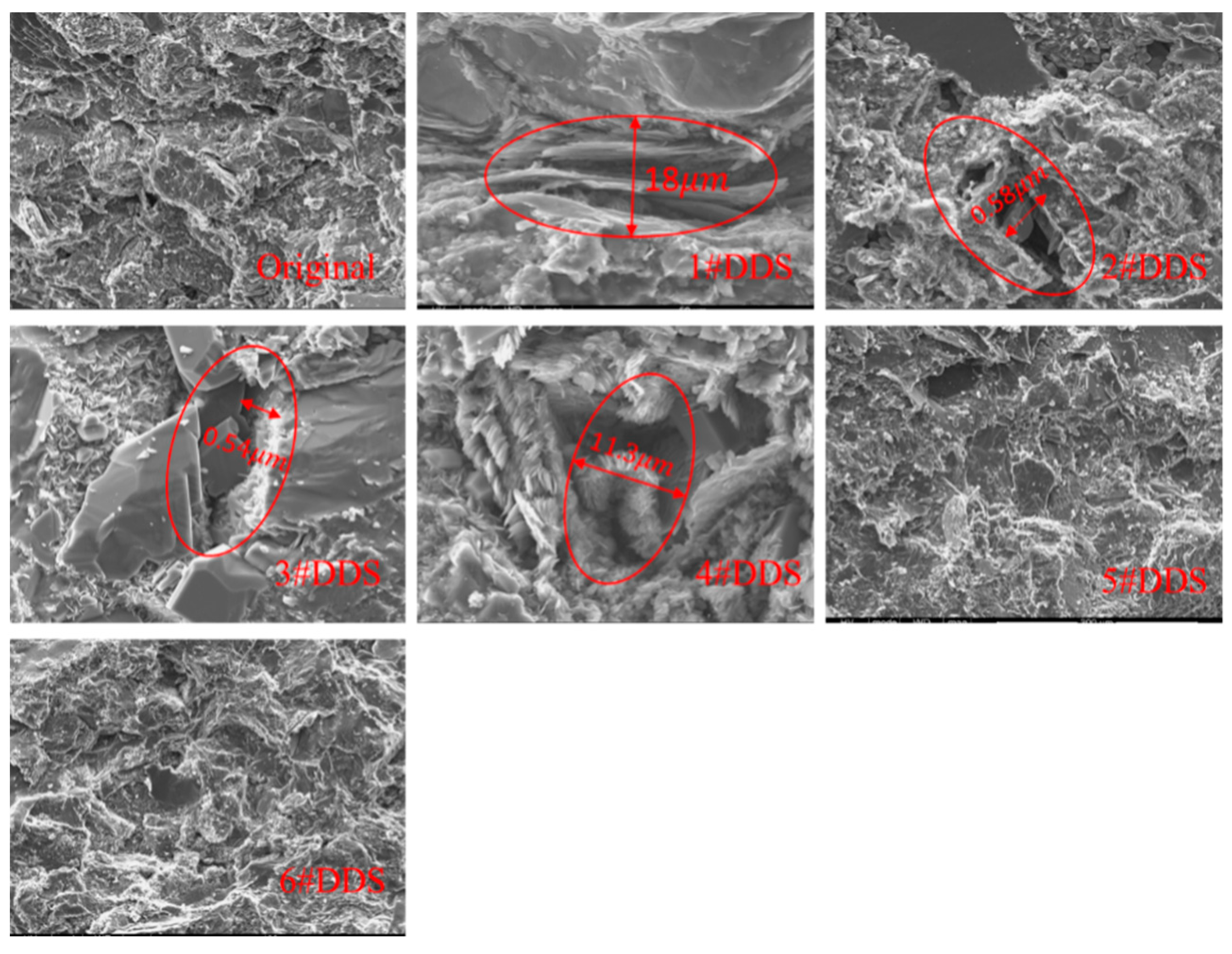
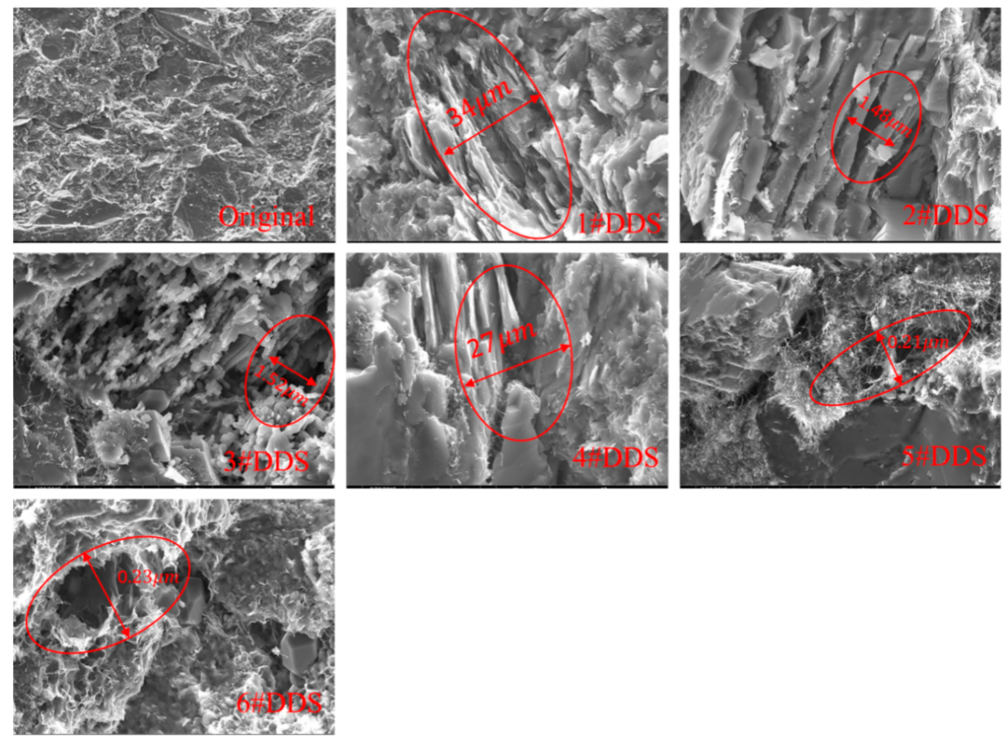
3.1. Microstructural Deformation under Stress Differences

As indicated in Sample 1 and Sample 2, it can be seen that only one main fracture was created when the horizontal stress difference was 4 MPa, while four induced fractures were created when the horizontal principal stress difference was 2.0 MPa. The DDS monitoring results indicate that the displacement near the wellbore was much larger than the others. At DDS #1, the displacements in Sample 1 and Sample 2 were 3.24 mm and 2.91 mm, and the total frequencies were 381 and 358. The displacements and total frequencies of the other five in Sample 1 were also higher than those in Sample 2. To further understand the microscopic pore throat deformation mechanism and mechanical property change characteristics, the rock samples located at the DDSs were drilled to conduct computed tomography (CT) scanning and a rock mechanical test. Figure 8 shows the CT scanning results of different locations in Sample 1. According to the results, the original pore throat structure was severely damaged at DDSs #1 and #4, and the obvious microcracks appeared. Meanwhile, the degrees of damage at DDSs #2 and #3 were much lower than at DDS #1 and further reduced at DDS #5 and #6.

To further understand the rock mechanical changes before and after hydraulic fracturing in Sample 1, six rock samples with a size of Ø25 × 50 mm were drilled at the DDSs, and the confined pressure was 30 MPa. Figure 9 shows the rock mechanical test results of Sample 1. We took the rock mechanical properties of the original rock as the standard. In the experiments, the compressive strength of the original rock and Young’s modulus were 150.93 MPa and 37.88 GPa, respectively. After the hydraulic fracturing experiment, the compressive strength and Young’s modulus for DDS #1 were 92.61 MPa and 24.73 GPa, decreases of 38.64% and 34.71%, respectively. The compressive strength and Young’s modulus for DDS #2 were 109.54 MPa and 28.61 GPa, decreases of 27.42% and 24.47%, respectively. For the rock sample at DDS #3, the compressive strength and Young’s modulus were 108.47 MPa and 28.54 GPa, decreases of 28.13% and 24.66%, respectively. For DDS #4, the compressive strength and Young’s modulus were close to that for DDS #1, decreasing to 95.89 MPa and 24.92 MPa, respectively. For the rock samples at DDS #4 and #6, the rock mechanical properties experienced a slight decrease with compressive strength values of 143.62 MPa and 145.37 MPa, respectively, and Young’s modulus values of 35.41 GPa and 35.46 GPa, respectively. Combined with Figure 8, it can be found that the significant structural change in the pore throat contributed to a sharp decrease in the compressive strength and Young’s modulus. Due to the pore throat structure being severely damaged in DDSs #1 and #4, the compressive strength and Young’s modulus also experienced a sharp decrease.

Figure 10 shows the CT scanning results of different locations in Sample 2. As indicated by DDS #1, the pore throat structure experienced a severe change, but the damage degree was significantly lower than that at DDS #1 in Sample 1. As shown in Figure 8, the created fracture width caused by the pore throat structure change was 26 μm, while it decreased to 18 μm, a decrease of 30.77%. The created fracture width at DDS #4 was 11.3 μm, a decrease of 19.29%. At DDSs #2 and #3 in Sample 2, the created fracture width also experienced a slight decrease.

Figure 11 shows the rock mechanical test results of Sample 2. We took the original rock as the standard with a Young’s modulus and compressive strength of 37.64 GPa and 150.62 MPa, respectively. After the hydraulic fracturing, the Young’s modulus and compressive strength for DDS #1 decreased to 25.76 GPa and 94.21 MPa, decreases of 37.45% and 31.56%, respectively. For DDS #2 and #3, the compressive strength decreased to 113.51 MPa and 114.71 MPa, decreases of 24.64% and 23.84%, respectively, and the Young’s modulus reduced to 31.47 GPa and 31.78 GPa, respectively. For DDS #4, the Young’s modulus and compressive strength had dramatic decreases to 28.96 GPa and 102.27 MPa, decreases of 32.11% and 23.06%. DDSs #5 and #6 had slight decreases in the compressive strength to 142.65 MPa and 143.21 MPa, respectively, and in the Young’s modulus to 35.21 GPa and 35.18 GPa, respectively. Compared to Sample 1, the change degree of the rock mechanics’ properties was lower than that in Sample 1, and the change degree in the pore throat structure was also significantly weakened. The main reason for this was that, with the increase in the hydraulic fractures, the displacement in different locations had an obvious increase, which was the main reason for the deformation of the pore throat structure in the shale formation. The more severe the deformation was of the rock pore throat structure, the more severe the compression deformation and shear failure of the shale sample, and the more serious the degradation of the rock mechanics. Thus, the degradation of the rock mechanics in Sample 1 was higher than that in Sample 2.

3.2. Microstructural Deformation under Different Pumping Rates

The pumping rate was also an important factor affecting the fracture creation. Compared to Sample 1, four induced fractures were created, which was higher than that in Sample 1. We subjected the six rock samples located at the DDSs in Sample 3 to a CT scanning test, and the CT scanning results are shown in Figure 12. It was found that the six rock samples were all damaged to varying degrees, and the rock samples at DDSs #1 and #4 were damaged the most severely, with fracture widths of 34 μm and 27 μm, respectively. For DDS #2 and #3, it was found that some microfractures were formed, and the fracture widths were 1.48 μm and 1.52 μm, respectively. For DDSs #5 and #6, only a slight change in the pore throat structure occurred, and the fracture widths were 0.21 μm and 0.23 μm, respectively. Compared to Sample 1, it can be concluded that the damage degree in Sample 3 was much higher than that in Sample 1. As depicted in Figure 8, the pore throat structure hardly underwent deformation in DDSs #5 and #6, while some deformation still was found, as shown in Figure 12. In addition, the fracture width in Sample 3 was much wider than that in Sample 1.

Figure 13 shows the rock mechanical test results of Sample 3. We took the original rock as the standard with a Young’s modulus and compressive strength of 37.97 GPa and 150.87 MPa, respectively. The rock mechanical properties of the other six rock samples experienced significant decreases after the hydraulic fracturing. In the rock mechanical tests, the Young’s modulus and compressive strength decreased to 23.57 GPa and 89.74 MPa, decreases of 40.52% and 36.96%, respectively. For DDSs #2 and #3, the compressive strength values were reduced to 103.57 MPa and 104.21 MPa, respectively, and the Young’s modulus values dropped to 25.61 GPa and 25.73 GPa, respectively. As for DDS #4, the Young’s modulus and compressive strength experienced sharp reductions to 92.58 MPa and 27.62 GPa, reductions of 38.64% and 26.13%, respectively. DDSs #5 and #6 experienced slight decreases in the compressive strength, to 136.84 MPa and 136.51 MPa, respectively, and in the Young’s modulus, to 34.24 GPa and 34.08 GPa, respectively. Compared to Sample 1, it can be concluded that the degradation of the rock mechanics in Sample 3 was much more serious than that in Sample 1. The main reason was that the high pumping rate was good for improving the net pressure in the fracture, thus creating high pressure on the fracture surface, and causing the deformation of the pore throat structure and the generation of microfractures, which contributed to the degradation of the rock mechanics in Sample 3.

3.3. Microstructural Deformation under Different Viscosities of Fracturing Fluid

To understand the microstructural deformation of rock under different viscosities of fracturing fluid, six rock samples located at the DDSs in Sample 4 underwent CT scanning, and the CT scanning results are shown in Figure 14. From the CT scanning tests, it was found that a fracture with a width of 47 μm was created at DDS #1, and a fracture with a width of 33 μm was created at DDS #4. For DDSs #2 and #3, two fractures with fracture widths of 24 μm and 26 μm were generated, respectively. Interestingly, no fractures were found at DDSs #5 and #6 DDS. Figure 15 shows the rock mechanical property distribution after hydraulic fracturing in Sample 4. As indicated in Figure 15, it was found that the Young’s modulus and compressive strength of the original rock sample were 155.08 MPa and 37.53 GPa, respectively. Taking the original rock as the standard, the Young’s modulus and compressive strength of the rock sample at DDS #1 were reduced to 86.47 MPa and 24.17 GPa, reductions of 44.24% and 35.59%, respectively. For DDS#2 and #3, the compressive strength decreased to 104.33 MPa and 105.27 MPa, reductions of 32.73% and 32.12%, respectively, compared to the original rock. The Young’s modulus also experienced decreases to 25.74 GPa and 25.86 GPa, respectively. For DDS#4, the Young’s modulus and compressive strength were 92.61 MPa and 25.17 GPa, reductions of 40.28% and 32.93%, respectively. For DDS #5 and #6, the compressive strengths decreased to 152.42 MPa and 152.67 MPa, respectively, and the Young’s modulus values decreased to 36.84 GPa and 36.89 GPa, respectively. Combined with Figure 14, it can be seen that the fractures were only created in the rock samples at DDSs #1, #2, #3, and #4; so, the rock mechanics experienced degradation. The main reason for this was that the high viscosity of the fracturing fluid effectively reduced the filtration of the fracturing fluid into the rock matrix, which hindered the generation of induced fractures. It also maintained a high net pressure inside the fracture. The high net pressure promoted the compression deformation of the fracture wall, causing severe deformation of the fracture wall near the injection point, leading to changes in the pore throat structure of the rock, and further leading to the degradation of the mechanical properties.

3.4. Failure Mode Determination

To determine the failure mode during the hydraulic fracture propagation, a numerical model was established to simulate the hydraulic fracturing process. In the simulation, the tensile failure and shear failure criteria were considered in the model [31,32,33,34]. The governing equations were as follows.

In the simulation, the relationship between the stress and strain can be described as follows.

$${\sigma }_{ij,j}+b_i-\rho u_{i,tt}-\alpha u_{i,t}=0$$

(1)

$${\sigma }_{ij}=D_{ijst}{\epsilon }_{st}$$

(2)

$${\epsilon }_{ij}=\frac{1}{2}(u_{i,j}+u_{j,i}),$$

(3)

where ${\sigma }_{ij}$ is the Cauchy tensor; $b_i$ is the body force; $\rho$ is the density of rock; $\alpha$ is the damping coefficient; $u_i$ is the displacement; ${\epsilon }_{ij}$ is the strain; $D_{ijst}$ is the Hooke tensor.

During the simulation, the fluid flow within the fracture is as follows:

$$q=-\frac{w^3}{12\mu }\frac{\partial p}{\partial s}$$

(4)

The local continuity equation in the fracture can be described as

$$\frac{\partial w}{\partial t}+\frac{\partial q}{\partial s}+q_l=0.$$

(5)

The global mass conservation equation can be stated as

$$Q_0={\displaystyle \underset{\Omega }{\int }\frac{\Delta w}{\Delta t}}ds+{\displaystyle \underset{\Omega }{\int }{q}_l}ds,$$

(6)

where $p$ is the fluid pressure; μ is the viscosity; $w$ is the fracture width; t is the time; q is the volume flow; $q_l$ is the filtration loss of the fracturing fluid.

Due to the injection of the fracturing fluid, the pressure at the perforation significantly increased, and the elements had tensile failure or shear failure; namely, the maximum principal stress reached the tensile strength of the rock, and tensile failure occurred, or the Mohr–Coulomb criterion was met, and shear failure occurred. The failure criterion is demonstrated as follows.

$$-{\sigma }_1>{\sigma }_T$$

(7)

$$\left|\tau \right|>{\tau }_0+\tan \phi {{\sigma }^{\prime }}_n,$$

(8)

where ${\sigma }_1$ is the maximum principle stress; ${\sigma }_T$ is the tensile strength of the rock; ${\tau }_0$ is the cohesion strength of the rock; φ is the angle of internal friction; σ′n is the shearing stress.

Based on the model, the displacement caused by hydraulic fracturing was calculated. Figure 16 shows the displacement located as DDSs #1, #2, #4, and #5 in Sample 1, Sample 2, Sample 3, and Sample 4 under three different situations; namely, only tensile failure or shear failure was considered, or the tensile failure and shear failure were considered together. Combined with

Table 2. Percentage of failure in different samples.

Samples	DDS	Tensile Failure Percentage/%	Shear Failure Percentage/%
Sample 1	DDS #1	73.51	26.39
	DDS #2	68.16	32.84
	DDS #4	71.24	28.76
	DDS #5	54.52	44.48
Sample 2	DDS #1	81.24	18.76
	DDS #2	67.24	32.76
	DDS #4	71.83	28.17
	DDS #5	56.23	44.77
Sample 3	DDS #1	86.15	13.85
	DDS #2	56.34	43.66
	DDS #4	68.27	31.73
	DDS #5	38.92	61.08
Sample 4	DDS #1	71.26	28.74
	DDS #2	61.24	38.76
	DDS #4	68.12	31.88
	DDS #5	39.45	60.55

, it can be seen that tensile failure was the main failure mode near the wellbore. As indicated in Table 2, it can be seen that the average percentage of tensile failure was much higher than that of shear failure. With the increase in the complex fracture network, the percentage of shear failure experienced a significant increase. Comparing Sample 1 and Sample 3, it was found that the average percentage of shear failure increased from 33.12% to 37.58% in Sample 1. In addition, the percentage of shear failure at DDS #5 was much higher than at the other three DDSs, which indicates that with the increase in the distance between the measurement point and the injection point, the likelihood of rock shear failure also increased significantly. Due to the porous medium of the reservoir rock, the enormous pressure generated during the injection of the fracturing fluid caused significant deformation of the fracture surface, leading to tensile failure of the rock. The displacement generated by the hydraulic surface may have also caused the rock pore-throat structure deformation in the far-field zone. As the distance between the measurement point and the injection point gradually increased, the influence of the normal stress on the crack wall gradually weakened, and the degree of shear stress reduction compared to normal stress was significantly reduced; hence, the proportion of shear failure gradually increased.

4. Conclusions

Based on the experiments and simulations, the displacement and failure modes were determined during hydraulic fracturing, and the factors affecting the hydraulic fracture distribution were discussed. The conclusions are drawn as follows.

(1)

The displacement of rock caused by hydraulic fracturing can make the pore throat structure change during hydraulic fracturing, and it also can reduce the rock mechanical strength in an unstimulated zone. According to the experimental results, it can be concluded that with the increase in the branch fractures, the displacement monitored by the DDSs also showed increases, the pore throat structure experienced severe changes, and the rock mechanical strength also experienced a sharp decrease.

(2)

From the simulation results, it was found that tensile failure was the main failure mode near the wellbore, and the percentage of shear failure experienced an obvious increase when the measurement point was further from the injection point.

(3)

Due to the porous medium of the reservoir rock, the enormous pressure generated during the injection of the fracturing fluid caused significant deformation of the fracture surface, leading to the tensile failure of the rock. The displacement of the fracture surface caused by the fracturing fluid injection also led to the deformation of the pore throat structure; thus, the shear failure increased when the measurement point was further from the injection point.

References

1. Zou, C.; Zhu, R.; Dong, D.; Wu, S. Scientific and technological progress, development strategy and policy suggestion regarding shale oil and gas. Acta Pet. Sin. 2022, 43, 1675–1686. [Google Scholar]
2. Jiang, T.; Bian, X.; Wang, H.; Li, S.; Jia, C.; Liu, H.; Sun, H. Volume fracturing of deep shale gas horizontal wells. Nat. Gas Ind. 2017, 37, 90–96. [Google Scholar] [CrossRef]
3. Wei, Y.; Jia, A.; He, D.; Junlei, W. Comparative analysis of development characteristics and technologies between shale gas and tight gas in China. Nat. Gas Ind. 2017, 37, 43–52. [Google Scholar]
4. Peng, T.; Yan, J.; Bing, H.; Yingcao, Z.; Ruxin, Z.; Zhi, C.; Meng, F. Laboratory investigation of shale rock to identify fracture propagation in vertical direction to bedding. J. Geophys. Eng. 2018, 15, 696. [Google Scholar] [CrossRef]
5. Liu, Y.; Zheng, X.; Peng, X.; Zhang, Y.; Chen, H.; He, J. Influence of natural fractures on propagation of hydraulic fractures in tight reservoirs during hydraulic fracturing. Mar. Pet. Geol. 2022, 138, 105505. [Google Scholar] [CrossRef]
6. Al-Rubaye, A.; Mahmud, H.K.B. A numerical investigation on the performance of hydraulic fracturing in naturally fractured gas reservoirs based on stimulated rock volume. J. Pet. Explor. Prod. Technol. 2020, 10, 3333–3345. [Google Scholar] [CrossRef]
7. Liu, Z.; Chen, M.; Zhang, G. Analysis of the Influence of a Natural Fracture Network on Hydraulic Fracture Propagation in Carbonate Formations. Rock Mech. Rock Eng. 2014, 47, 575–587. [Google Scholar] [CrossRef]
8. Li, Q.; Wang, F.; Wang, Y.; Forson, K.; Cao, L.; Zhang, C.; Zhou, C.; Zhao, B.; Chen, J. Experimental investigation on the high-pressure sand suspension and adsorption capacity of guar gum fracturing fluid in low-permeability shale reservoirs: Factor analysis and mechanism disclosure. Environ. Sci. Pollut. Res. 2022, 29, 53050–53062. [Google Scholar] [CrossRef]
9. Zou, Y.; Ma, X.; Zhang, S.; Zhou, T.; Li, H. Experimental investigation into the influence of bedding plane on hydraulic fracture network propagation in shale formations. Rock Mech. Rock Eng. 2016, 49, 3597–3614. [Google Scholar]
10. Li, X.; Hofmann, H.; Yoshioka, K.; Luo, Y.; Liang, Y. Phase-Field Modelling of Interactions Between Hydraulic Fractures and Natural Fractures. Rock Mech. Rock Eng. 2022, 55, 6227–6247. [Google Scholar] [CrossRef]
11. Zhang, F.; Dontsov, E.; Mack, M. Fully coupled simulation of a hydraulic fracture interacting with natural fractures with a hybrid discrete-continuum method. Int. J. Numer. Anal. Methods Geomech. 2017, 41, 1430–1452. [Google Scholar] [CrossRef]
12. Wu, M.; Wang, W.; Song, Z.; Liu, B.; Feng, C. Exploring the influence of heterogeneity on hydraulic fracturing based on the combined finite–discrete method. Eng. Fract. Mech. 2021, 252, 107835. [Google Scholar] [CrossRef]
13. Cheng, W.; Jin, Y.; Lin, Q.; Chen, M.; Zhang, Y.; Diao, C.; Hou, B. Experimental Investigation About Influence of Pre-existing Fracture on Hydraulic Fracture Propagation Under Tri-axial Stresses. Geotech. Geol. Eng. 2015, 33, 467–473. [Google Scholar] [CrossRef]
14. Tan, P.; Chen, G.; Wang, Q.; Zhao, Q.; Chen, Z.; Xiang, D.; Xu, C.; Feng, X.; Zhai, W.; Yang, Z.; et al. Simulation of hydraulic fracture initiation and propagation for glutenite formations based on discrete element method. Front. Earth Sci. 2023, 10, 1116492. [Google Scholar] [CrossRef]
15. Fu, L.; Hu, J.; Zhang, Y. Study on fracture initiation pressure of a horizontal well considering the influence of stress shadow in tight sand reservoirs. J. Nat. Gas Sci. Eng. 2022, 101, 104537. [Google Scholar] [CrossRef]
16. Chen, Y.; Zhang, Q.; He, J.; Liu, H.; Zhao, Z.; Du, S.; Wang, B. Pressure transient analysis of volume-fractured vertical well with complex fracture network in the reservoir. J. Nat. Gas Sci. Eng. 2022, 101, 104556. [Google Scholar] [CrossRef]
17. Zheng, H.; Pu, C.; Xu, E.; Sun, C. Numerical investigation on the effect of well interference on hydraulic fracture propagation in shale formation. Eng. Fract. Mech. 2020, 228, 106932. [Google Scholar] [CrossRef]
18. Zheng, H.; Pu, C.; Sun, C. Numerical investigation on the hydraulic fracture propagation based on combined finite-discrete element method. J. Struct. Geol. 2020, 130, 103926. [Google Scholar] [CrossRef]
19. Taheri-Shakib, J.; Ghaderi, A.; Hosseini, S.; Hashemi, A. Debonding and coalescence in the interaction between hydraulic and natural fracture: Accounting for the effect of leak-off. J. Nat. Gas Sci. Eng. 2016, 36, 454–462. [Google Scholar] [CrossRef]
20. Guo, T.; Zhang, S.; Qu, Z. Experimental study of hydraulic fracturing for shale by Stimulated reservoir volume. Fuel 2014, 128, 373–380. [Google Scholar] [CrossRef]
21. Heng, S.; Liu, X.; Li, X.; Zhang, X.; Yang, C. Experimental and numerical study on the non-planar propagation of hydraulic fractures in shale. J. Pet. Sci. Eng. 2019, 179, 410–426. [Google Scholar] [CrossRef]
22. Yushi, Z.; Shicheng, Z.; Tong, Z.; Xiang, Z.; Tiankui, G. Experimental Investigation into Hydraulic Fracture Network Propagation in Gas Shales Using CT Scanning Technology. Rock Mech. Rock Eng. 2016, 49, 33–45. [Google Scholar] [CrossRef]
23. Stanchits, S.; Burghardt, J.; Surdi, A. Hydraulic Fracturing of Heterogeneous Rock Monitored by Acoustic Emission. Rock Mech. Rock Eng. 2015, 48, 2513–2527. [Google Scholar] [CrossRef]
24. Cruz, F.; Roehl, D.; Vargas, E.D.A. An XFEM element to model intersections between hydraulic and natural fractures in porous rocks. Int. J. Rock Mech. Min. Sci. 2018, 112, 385–397. [Google Scholar] [CrossRef]
25. Cheng, W.; Jin, Y.; Chen, M. Reactivation mechanism of natural fractures by hydraulic fracturing in naturally fractured shale reservoirs. J. Nat. Gas Sci. Eng. 2015, 23, 431–439. [Google Scholar] [CrossRef]
26. Fatahi, H.; Hossain, M.M.; Sarmadivaleh, M. Numerical and experimental investigation of the interaction of natural and propagated hydraulic fracture. J. Nat. Gas Sci. Eng. 2017, 37, 409–424. [Google Scholar] [CrossRef]
27. Rysak, B.; Gale, J.F.; Laubach, S.E.; Ferrill, D.A. Mechanisms for the Generation of Complex Fracture Networks: Observations from Slant Core, Analog Models, and Outcrop. Front. Earth Sci. 2022, 10, 848012. [Google Scholar] [CrossRef]
28. Zheng, Y.; He, R.; Huang, L.; Bai, Y.; Wang, C.; Chen, W.; Wang, W. Exploring the effect of engineering parameters on the penetration of hydraulic fractures through bedding planes in different propagation regimes. Comput. Geotech. 2022, 146, 104736. [Google Scholar] [CrossRef]
29. Dehghan, A.N. An experimental investigation into the influence of pre-existing natural fracture on the behavior and length of propagating hydraulic fracture. Eng. Fract. Mech. 2020, 240, 107330. [Google Scholar] [CrossRef]
30. Wu, S.; Li, T.; Ge, H.; Wang, X.; Li, N.; Zou, Y. Shear-tensile fractures in hydraulic fracturing network of layered shale. J. Pet. Sci. Eng. 2019, 183, 106428. [Google Scholar] [CrossRef]
31. Sun, C.; Zheng, H.; Liu, W.D.; Lu, W. Numerical simulation analysis of vertical propagation of hydraulic fracture in bedding plane. Eng. Fract. Mech. 2020, 232, 107056. [Google Scholar] [CrossRef]
32. Joseph, P.F.; Loghin, A. Letter to the Editor of Engineering Fracture Mechanics. Eng. Fract. Mech. 2020, 232, 107049. [Google Scholar] [CrossRef]
33. Shi, S.; Zheng, H.; Kong, H.; Luo, Y.; Chen, F. Study on the failure mechanism in shale-sand formation based on hybrid finite-discrete element method. Eng. Fract. Mech. 2022, 272, 108718. [Google Scholar] [CrossRef]
34. Wang, L. Study on the influence of temperature on fracture propagation in ultra-deep shale formation. Eng. Fract. Mech. 2023, 281, 109118. [Google Scholar] [CrossRef]
Figure 1. The distribution sketch of the distributed displacement sensors in the experiment.
Processes 11 02931 g001
Figure 2. Fracture geometry under different situations (rock sample picture).
Processes 11 02931 g002
Figure 3. Fracture geometry under different situations (the yellow dashed line is the main fracture, and the white dashed line is the induced fracture).
Processes 11 02931 g003
Figure 4. The signal distribution of the sensors in Sample 1. 1 #–6 # are displacement change monitored in six distributed displacement sensors.
Processes 11 02931 g004
Figure 5. The signal distribution of the sensors in Sample 2. 1 #–6 # are displacement change monitored in six distributed displacement sensors.
Processes 11 02931 g005
Figure 6. The signal distribution of the sensors in Sample 3. 1 #–6 # are displacement change monitored in six distributed displacement sensors.
Processes 11 02931 g006
Figure 7. The signal distribution of the sensors in Sample 4. 1 #–6 # are displacement change monitored in six distributed displacement sensors.
Processes 11 02931 g007
Figure 8. Microstructure changes before and after the hydraulic fracturing in Sample 1.
Processes 11 02931 g008
Figure 9. Rock mechanical property distribution after hydraulic fracturing in Sample 1.
Processes 11 02931 g009
Figure 10. The microstructure change before and after the hydraulic fracturing in Sample 2.
Processes 11 02931 g010
Figure 11. Rock mechanical property distribution after hydraulic fracturing in Sample 2.
Processes 11 02931 g011
Figure 12. Microstructure changes before and after hydraulic fracturing in Sample 3.
Processes 11 02931 g012
Figure 13. Rock mechanical property distribution after hydraulic fracturing in Sample 3.
Processes 11 02931 g013
Figure 14. Microstructure changes before and after hydraulic fracturing in Sample 4.
Processes 11 02931 g014
Figure 15. Rock mechanical property distribution after hydraulic fracturing in Sample 4.
Processes 11 02931 g015
Figure 16. Displacement under different failure modes in different samples. S-1-1–S-4-5 is the Displacement monitored by sensors at different positions in four rock samples. The first number represents the sample number and the second number represents the sensor number.
Processes 11 02931 g016