1. Introduction
Process optimization is the iterative refinement of a system or process to enhance its efficiency and adaptability. It adjusts parameters to achieve optimal outputs with fewer resources and waste. The goal is to maximize metrics like yield or efficiency within set constraints, often using tools such as computational algorithms and real-time monitoring [
1].
In the context of reaction systems, process optimization generally aims to maximize feed rate and/or conversion in response to changes in feed quality, ambient conditions, or market demands, all while adhering to as many constraints as possible [
2].
The phrase “smart manufacturing” was first coined by the Smart Manufacturing Leadership Coalition (SMLC) [
3]. They defined smart manufacturing as an advanced form of manufacturing that (a) relies on the integration and coordination of information, automation, computation, software, sensing, and networking, and (b) utilizes state-of-the-art materials and emerging capabilities stemming from both the physical and biological sciences. This definition encompasses not only innovative methods to produce existing products but also the production of novel products derived from cutting-edge technologies.
Moreover, a comprehensive review of standards and projected scenarios in smart manufacturing process and system automation was undertaken [
4]. This review offered an overview of the prevailing manufacturing automation standards, with a focus on integrated processes tailored for mass personalization and agile automation. The authors delineated the vision of smart manufacturing and its prerequisites for upcoming automation. In response to the demand for efficient production of personalized products, they explored scenarios that amalgamate existing standards.
Smart manufacturing represents a profound integration of networked, information-driven technologies across the manufacturing and supply chain spectrum. It emphasizes synchronization, integrated performance metrics, and cyber-physical–workforce dynamics. This approach catalyzes a transformative shift towards customer-centric economics, streamlined enterprise performance, real-time materials engineering, and demand-responsive supply chains. IT-enhanced smart factories and networks bolster national priorities, enhancing global competitiveness, fostering sustainable jobs, elevating performance, and driving innovative manufacturing [
5].
The relentless pursuit of advancements in equipment, operations, and controls is pivotal for process optimization. This pursuit aims to enhance productivity, curtail expenses, and bolster quality. Equipment optimization [
6,
7,
8,
9,
10] necessitates regular maintenance, equipment upgrades, adoption of cutting-edge technology and designs, and the minimization of maintenance downtime. In contrast, operations optimization [
11,
12,
13,
14,
15] focuses on refining processes, diminishing waste, and streamlining the flow of materials and information. Controls optimization [
16,
17,
18,
19,
20] leverages advanced control systems, sensors, and automation to fine-tune the performance of equipment and processes. A holistic optimization of these domains can amplify efficiency, curtail costs, elevate quality, boost competitiveness, and enhance customer satisfaction. Nevertheless, optimization is a perpetual endeavor, and its success hinges on continuous refinement. Periodic evaluations and process enhancements are instrumental in optimizing the performance, efficiency, and profitability of manufacturing operations.
Numerous studies have endeavored to tweak process parameters to achieve specific optimization goals or minimize certain process specifications all while adhering to constraints. These studies span a plethora of sectors, including but not limited to chemical [
21,
22,
23,
24,
25], energy [
26,
27,
28,
29], business [
30,
31,
32,
33], agriculture [
34,
35,
36,
37], medical [
38,
39,
40,
41], and manufacturing [
9,
42,
43,
44,
45,
46].
While smart manufacturing and Industry 4.0 are closely related and often used interchangeably in some contexts, they are not strictly synonymous. Smart manufacturing focuses on using advanced data analytics, automation, and other technologies to enhance manufacturing processes. On the other hand, Industry 4.0 represents the fourth industrial revolution, encompassing a broader range of technological advancements, including the Internet of Things (IoT), cyber-physical systems, and more, of which smart manufacturing is a significant component. Smart manufacturing [
5] harnesses avant-garde information and communication technologies to elevate manufacturing processes, enhance supply chain efficiency, and improve customer satisfaction. This paradigm encompasses real-time monitoring and control, integrated performance metrics, and holistic participation from the workforce. The advantages of smart manufacturing encompass heightened competitiveness, new types of job opportunities, elevated performance, and innovation within the manufacturing industry. While it is true that the automation aspect of smart manufacturing can reduce certain manual labor roles, it simultaneously creates specialized job opportunities. These include positions in system design, maintenance, data analysis, software development, quality assurance, system optimization, and cybersecurity. As manufacturing processes become more technologically advanced, there is a growing demand for skilled professionals who can design, implement, and maintain these sophisticated systems. Thus, smart manufacturing shifts the job landscape from traditional manual roles to more technologically centric positions.
The quintessence of smart manufacturing is the production of bespoke products efficiently and cost-effectively. A comprehensive study [
4] delved into contemporary guidelines for automating manufacturing processes and systems. It emphasized the paramountcy of seamless integration and the role of advanced automation in facilitating large-scale customization and reactive factory automation.
Smart manufacturing integrates Internet of Things (IoT) devices [
47,
48,
49,
50,
51,
52], cloud computing [
51,
53,
54,
55,
56], robotics [
57,
58,
59,
60], and artificial intelligence (AI) algorithms [
61,
62,
63,
64] to ensure real-time oversight and management of production processes.
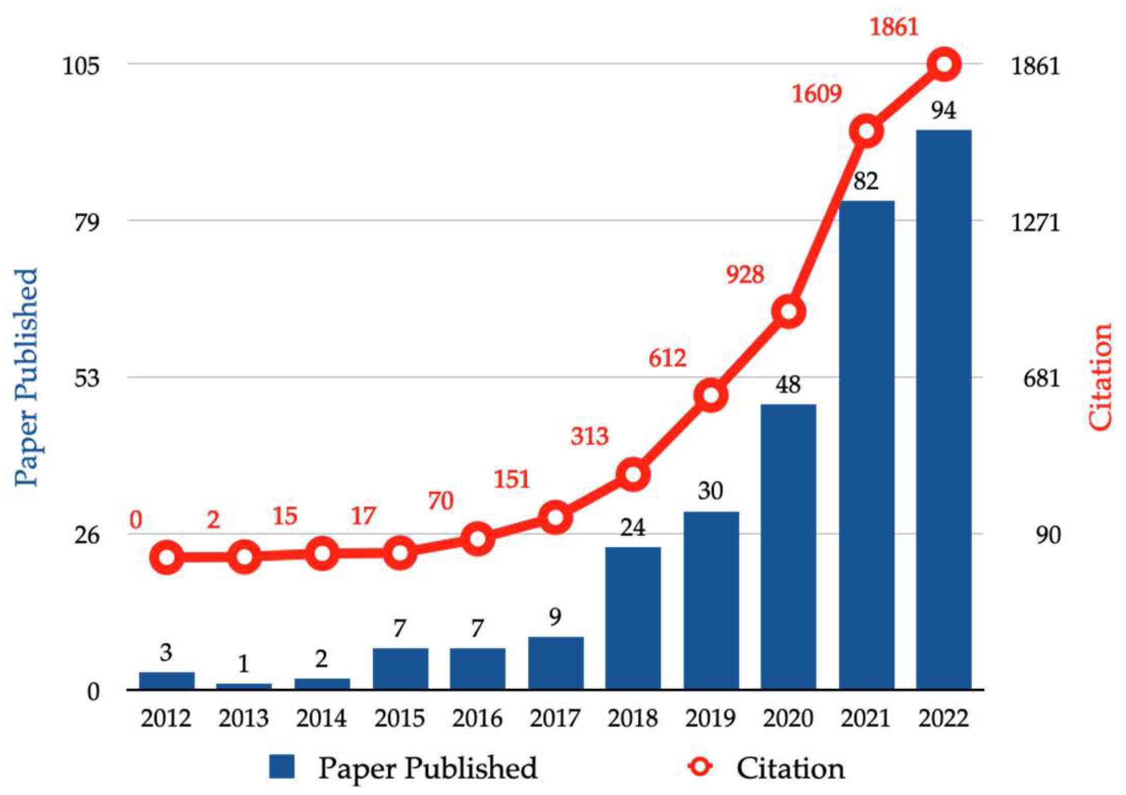
Numerous studies have explored the application of intelligent control in process optimization, examining the practical implementation of intelligent control principles. In the Web of Science database, topic searches scrutinize record fields, including title, abstract, author keywords, and Keywords Plus
®, for relevant terms. As
Figure 1 demonstrates, the past decade has witnessed a substantial increase in both publications and citations on this topic, indicating escalating interest among researchers and practitioners.
Figure 2 presents the distribution of papers across various subject areas and published during the past decade that relate to intelligent control and process optimization. Data indicate that computer science, electrical electronics, and telecommunications jointly account for 65% of total publications.
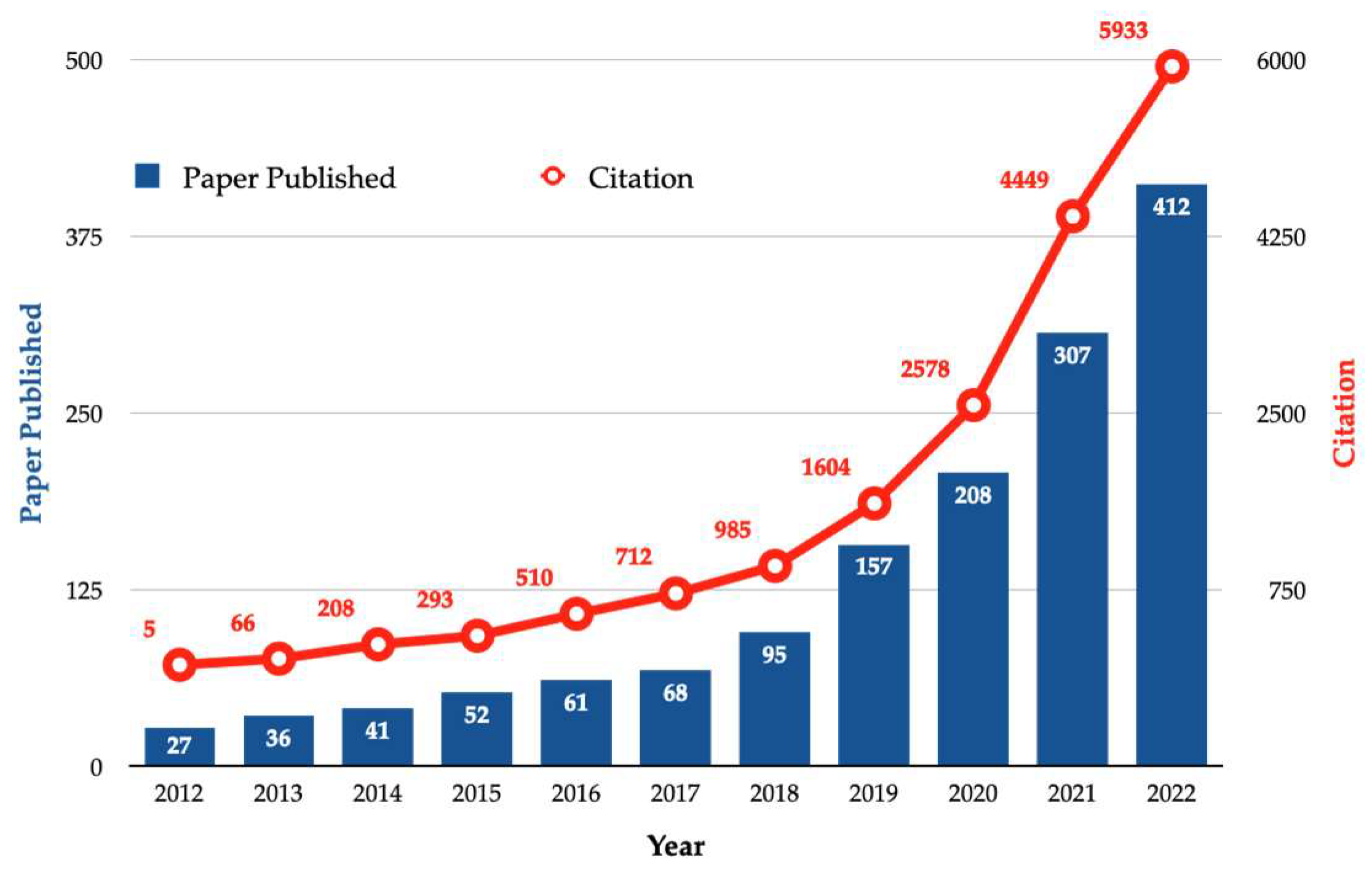
Figure 3 showcases the volume of papers and citations on intelligent control and smart manufacturing over the past decade, sourced from topic searches in the Web of Science database. A marked uptrend in both publications and citations is evident.
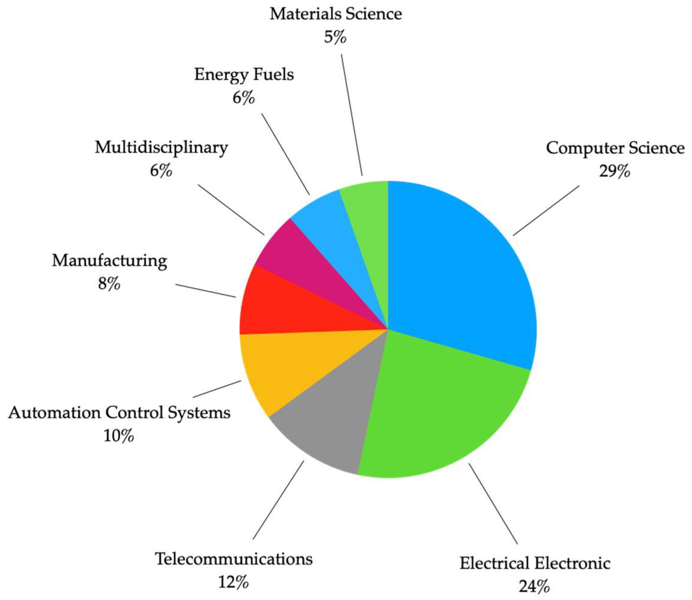
Figure 4 portrays the percentage distribution of papers related to intelligent control and smart manufacturing across various subject areas over the past decade. Notably, computer science, electrical electronics, material science, and manufacturing jointly comprise 67% of total publications.
This review aims to offer a contemporary discourse on intelligent control theory and its applications in process optimization and smart manufacturing. It delves into three intelligence approaches: inference intelligence (simulation-based), learning intelligence (modeling-based), and evolutionary intelligence (optimization-based). Specifically, the review evaluates these approaches in the context of process optimization, examining how equipment optimization, operational procedures, and control optimization influence optimal performance. Similarly, the review assesses these methodologies concerning their potential to achieve four primary objectives in smart manufacturing: curtailing product development cycles, cost reduction, production efficiency enhancement, and product quality improvement.
Figure 5 delineates the nuanced distinction between autonomous and automatic operations, emphasizing their approximation capabilities. This encompasses myriad factors, such as ambiguity, vagueness, generality, imprecision, uncertainty, fuzziness, belief (subjective probability), and plausibility, as elaborated in [
65]. While Industry 3.0 accentuates automatic operations and competitiveness via cost-cutting and leveraging affordable labor, Industry 4.0 emphasizes autonomous operations and enhancing value, potentially leading to price hikes due to the integration of machine intelligence. While Industry 4.0 emphasizes autonomous operation and competitiveness through value enhancement, which in some cases may lead to increased prices due to the integration of machine intelligence, it is essential to note that the economic implications can vary. Specifically, in regions where labor costs are high, the adoption of Industry 4.0 technologies might indeed lead to cost savings and potentially reduced prices for end products.
The faculty of approximation, emblematic of intelligence, is inherently a “soft” concept. “Soft computing” complements traditional AI in the domain of machine intelligence (or computational intelligence), underpinning intelligent control theory. Three predominant methodologies in this realm are fuzzy logic, neural networks, and genetic algorithms. As elucidated in [
65], these techniques draw parallels with biological phenomena:
- -
Fuzzy logic emulates inference intelligence, striving to mirror human cognition and the associated reasoning mechanisms;
- -
Neural networks inspired by learning intelligence, offer a rudimentary representation of brain neuron structures;
- -
Genetic algorithms echoing evolutionary intelligence, employ mechanisms akin to biological evolutionary processes.
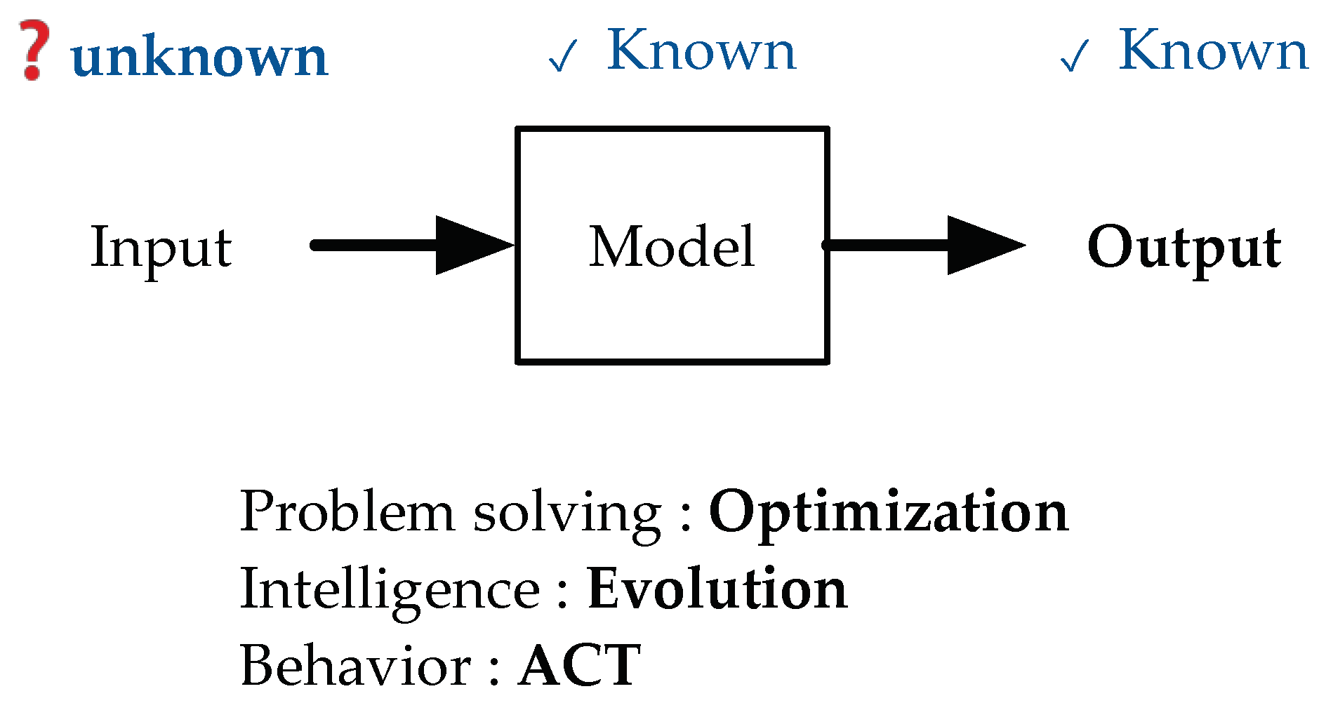
Table 1 showcases a system or process diagram comprising three elements: input, model, and output. It also details their interrelation with approach, intelligence, and behavior. In engineering, problem-solving typically encompasses three primary stages: simulation, modeling, and optimization. During simulation, the goal is to determine the outputs based on the inputs, aligning with inference intelligence and the SEE behavior. In the modeling phase, the objective is to discern the relationship between input and output, aligning with learning intelligence and the THINK behavior. Finally, optimization seeks the input(s) that yield the desired output, corresponding to evolutionary intelligence and the ACT behavior.
Figure 6 illustrates the hierarchical control architecture utilized in both process optimization and smart manufacturing systems, often termed supervisory control. High-level tasks define the system’s objectives and guide its overarching decision-making processes. Conversely, low-level tasks manage the system’s execution, addressing specific functional requirements like component design, algorithm execution, and resource management. Distributing tasks between high and low levels ensure a clear responsibility demarcation, promoting a modular and scalable system. This structure also streamlines problem diagnosis and resolution since each component can be individually addressed without affecting others. This supervisor control architecture employs conventional crisp techniques for low-level direct control. In contrast, upper levels handle supervisory tasks such as process monitoring, performance assessment, tuning, adaptation, and restructuring. The distributed architecture in
Figure 6 denotes a system design where components are dispersed across multiple locations, operating autonomously. The components exchange data and communicate via a network, devoid of a central point of control. Conversely, a centralized architecture design centralizes component control, with all components communicating through a singular communication point, managed and regulated by the central authority.
In hierarchical architectures, ensuring optimal and secure control techniques for nonlinear systems is paramount, especially when these systems are exposed to various external disturbances and attacks. Several methodologies have been proposed to address these challenges, emphasizing system stability and efficiency [
66,
67,
68].
One notable approach utilizes the event-triggered adaptive dynamic programming (ETADP) algorithm, focusing on the decentralized control of interconnected nonlinear systems influenced by stochastic dynamics [
66]. Another method introduces a combination of an anti-attack control strategy and a decentralized adaptive self-triggered control (ASTC) mechanism. This is particularly tailored to manage the control challenges in nonlinear multiagent systems (MASs) that are vulnerable to denial-of-service (DoS) attacks over directed graphs [
67].
Furthermore, a comprehensive solution has been proposed that integrates a dynamic threshold adjustable event-triggering mechanism, a neural network-based observer, a dynamic surface control method, and the Nussbaum function. This approach is designed for an event-based adaptive decentralized output feedback control scheme, targeting interconnected systems affected by Bouc–Wen hysteresis and those with unmeasured system states [
68].
2. Inference Intelligence
The process of problem-solving through simulations entails using inputs to derive corresponding outputs, as depicted in
Figure 7. This is realized through an AI paradigm termed as inference intelligence, which seeks to emulate expert knowledge to facilitate approximate reasoning. The cycle associated with this approach is termed SEE, encompassing the perception of incomplete, imprecise, and fuzzy data.
Fuzzy logic (FL) is an algorithmic approach that harnesses imprecise and incomplete sensor data (as the known inputs in
Figure 7), combined with expert rule-based knowledge (the known model in
Figure 7), to make practical inferences (the unknown outputs in
Figure 7). Traditional binary logic, which allows only two states, falls short in addressing vague terms like “slow”, “near”, “speed up”, or “turn slightly right”. For these subjective and approximate situations commonly faced in intelligent machine-related problems, fuzzy logic provides a more pragmatic solution. It is built on if–then rules incorporating fuzzy descriptors, allowing for partial truths. Unlike conventional Boolean logic, which strictly adheres to true or false values, fuzzy logic accommodates shades of truth. Detailed insights are available in [
65], summarized as:
A fuzzy set
A’s mathematical representation is through a membership function, expressed as
Each element of A, symbolized by a point x on the real line ℜ, is mapped to a value ranging from 0 to 1, indicating x’s membership grade in A.
Membership functions amalgamate to form a fuzzy rule, exemplified as
If A1 and B1 then C1
If A2 and B2 then C2
The antecedent consists of two fuzzy states, A and B, while the consequent comprises two fuzzy actions, C1 and C2, linked through logical connectives.
Initially, a set of if–then rules with vague descriptors for both antecedent and consequent variables is established. The data,
D, undergoes initial processing as per
Typically, this corresponds to “fuzzification”, defining
D’s membership grades. The fuzzy inference
for a knowledge base
is then deduced using fuzzy-predicate approximate reasoning, represented by
The composition operator
is articulated as
The fuzzy rule base’s multidimensional membership function is symbolized by , while denotes the fuzzified data’s membership function. signifies the fuzzy inference’s membership function, and represents the context variables set used in aligning with the knowledge base.
A centroid method can then ascertain the crisp value
necessary for the action:
where
c denotes inference
I’s independent variable, while
S signifies the inference membership function’s support set or region of interest.
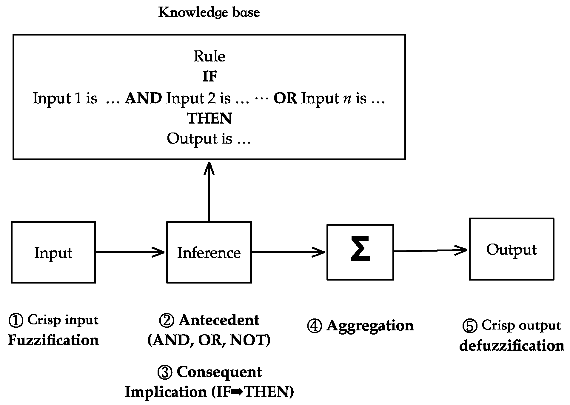
Figure 8 illustrates the comprehensive fuzzy inference process, encompassing (1) input variables’ fuzzification, (2) antecedent’s AND, OR, and NOT operators’ application, (3) consequent’s implication operator application (IF–THEN), (4) all rules’ consequents aggregation, and (5) output variable defuzzification.
Fuzzy logic’s versatility spans various domains, including control systems like process temperature regulation [
69], energy management [
70,
71], vacuum cleaning [
72], automatic transmission [
73], washing machines [
74], and pattern recognition tasks such as gait [
75], speckle [
76], and behavior [
77] pattern analysis. In image processing, it aids in image enhancement [
78,
79], segmentation [
80,
81], and registration [
82]). Within control systems, fuzzy logic control mirrors human decision-making processes.
In process optimization, a fuzzy logic control system ingests parameters like temperature, pressure, and flow rate. It then outputs control signals, adjusting process variables to achieve optimization objectives. Using fuzzy logic in process optimization primarily addresses inherent uncertainty and imprecision in the data. This involves applying fuzzy rules to correlate input values with control outputs, leveraging expert knowledge, and adjusting for optimal performance. Optimal performance hinges on three variables: equipment, control, and operation.
Table 2 delineates these variables across industries and processes.
In smart manufacturing, fuzzy logic control-process inputs like production data, process parameters, and machine status. The system analyzes these data, generating a control signal to modulate the production process, resulting in enhanced efficiency and efficacy.
Smart manufacturing’s objectives encompass accelerating product development, reducing costs, boosting production efficiency, and improving product quality.
Table 3 encapsulates these goals across industries and systems.
Type-2 fuzzy logic systems enhance type-1 fuzzy logic systems by allowing membership functions to be fuzzy sets. This introduces a more intricate layer to address greater uncertainties than type-1 systems [
107,
108].
Type-1 Fuzzy Sets: Traditional fuzzy logic uses a membership function to assign a membership grade between 0 and 1 to each object, indicating its belongingness to the set.
Type-2 Fuzzy Sets: Here, the membership grade itself is a fuzzy set within the [0, 1] interval, introducing uncertainty in membership degrees.
Type-2 fuzzy logic excels in handling heightened uncertainties. Where type-1 might falter due to noise and imprecision in real-world scenarios, type-2 offers a more nuanced approach. For instance, when experts provide varied membership functions for a concept, a type-2 system can encompass all these variations, capturing the inherent uncertainty.
In essence, while type-1 fuzzy logic adeptly manages uncertainty, type-2 offers a refined approach for scenarios with layered uncertainties.
3. Learning Intelligence
The objective of the modeling process, illustrated in
Figure 9, is to discern the relationship between input and output variables. A prime example of this approach is the neural network algorithm. It utilizes interconnected nodes to emulate complex systems without the necessity of an analytical model, mirroring the neural architecture of the human brain.
Neural networks are computational constructs comprising vast arrays of interconnected “neurons” that function in parallel, distributing processing tasks. Their design is inspired by the biological configuration of neurons in the human brain. Notable features include their capacity to approximate arbitrary nonlinear functions and undertake intricate nonlinear decision-making processes. A neural network is structured with nodes grouped into layers, interconnected by weighted elements termed synapses. In a biological context, dendrites receive information from other neurons, process it in the soma (cell body), and relay it to other neurons via an axon. The neural network’s prowess in learning from examples, approximating nonlinear functions, offering significant computational capabilities, and memory retention can be attributed to this biological parallel, underscoring its inherent “intelligence”.
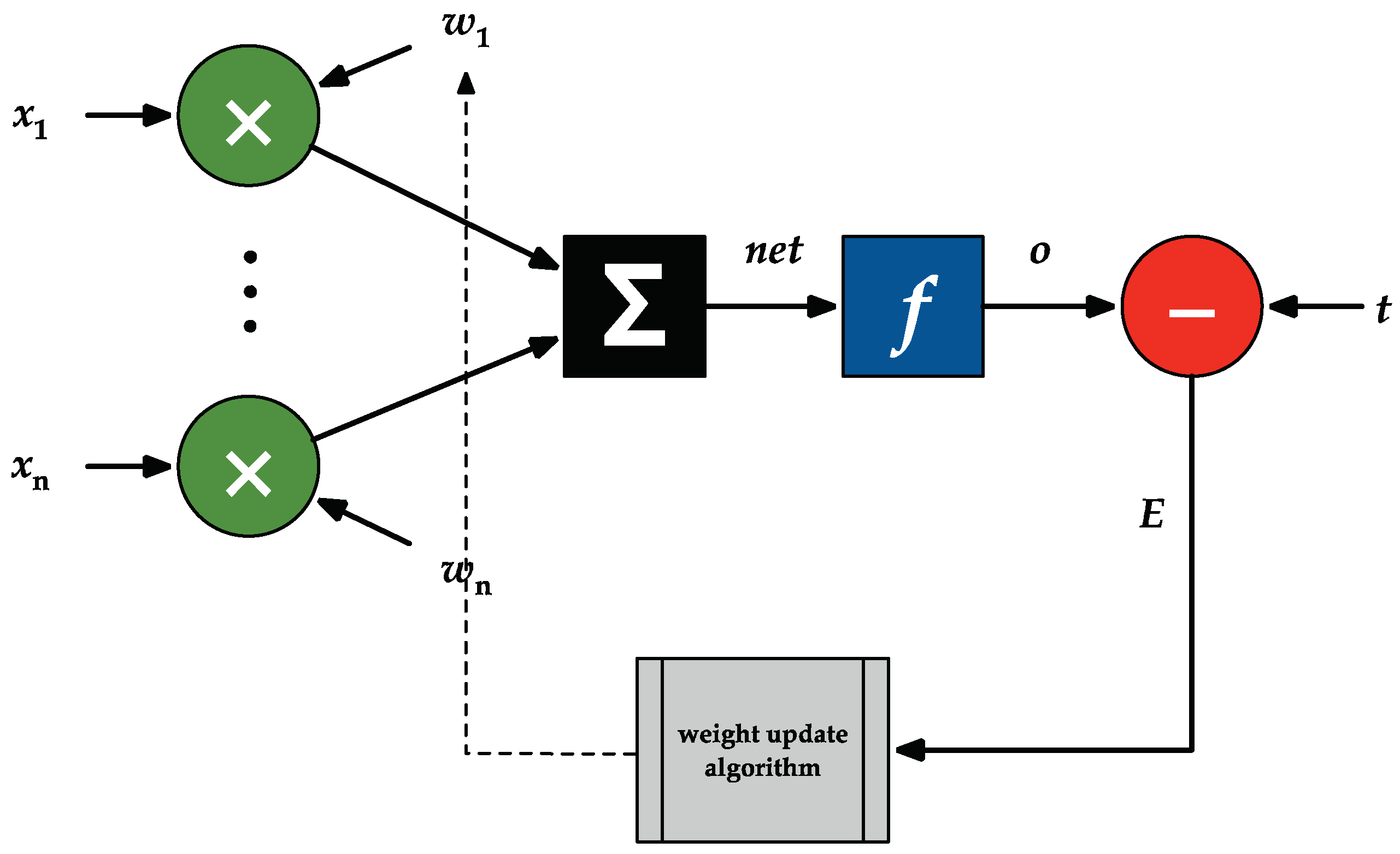
The perceptron, depicted in
Figure 10, represents one of the earliest neurons endowed with intelligent attributes and autonomous learning capabilities. Within the perceptron model, the weights
w1,
w2, …,
wn can adaptively adjust in response to fresh data, leveraging feedback and a learning rule.
The operational steps for a single neuron are as follows:
Initialization of weights: Assign small values (w1, w2, …, wn).
Feed-forward: Present the input vector x = (x1, x2, …, xn)T and obtain the output o using an activation function f as
- 3.
Error Calculation: Determine the error E as
- 4.
Training (Back-propagation): Ascertain the weight change wi by
- 5.
Weight Adjustment: Modify the weights based on:
The artificial neural network (ANN), termed the multiple layer perceptron (MLP), is depicted in
Figure 11. It comprises individual neurons as showcased in
Figure 10. Two architectural designs are presented: feed-forward (denoted by the black solid arrow), employing the back-propagation learning algorithm, and recurrent (highlighted with a red dashed arrow). Recurrent architectures include the Hopfield network, recurrent neural network (RNN), and time-delayed neural networks (TDNN). The methodology aligns with the single neuron concept, with further elaboration available in [
65].
3.1. Machine Learning
An artificial neural network (ANN) is a machine learning technique that employs computational methods to extract information directly from input/output data. Its performance can dynamically improve as the volume of training samples grows. During the network’s training phase, weight parameters at the neuron interconnection level are adjusted using one of three learning algorithms, as depicted in
Figure 12.
In supervised learning, the input is processed by the neural network to produce an output. The output is then contrasted with the target signal, yielding a cumulative error. This error informs the weight updates in the neural network through a supervised learning method. Two primary techniques exist:
- (1)
Classification, where the neural network yields a discrete response;
- (2)
Regression, where the response is continuous.
Unsupervised learning involves input processing by the neural network to generate an output. The weights in the neural network are then updated through unsupervised weight adjustment. The two main techniques follow:
- (1)
Clustering, which groups input data based on similarity patterns;
- (2)
Dimensionality reduction, which reduces the number of inputs or features.
Reinforcement learning uses the neural network’s input to produce an output. A reinforcement signal then guides the weight updates in the neural network. This method involves software agents acting within an environment to maximize cumulative reward, often discovering solutions via trial and error.
Originating in the early 1940s, ANNs were initially designed for pattern classification. Over time, their functionalities have expanded significantly. Today, ANNs find applications in a wide array of scientific and technological domains, especially within the industrial sector. They serve as pivotal tools for diverse applications such as process monitoring and control [
109], power systems [
110], medical diagnosis [
111], stock market prediction [
112], nuclear plant control [
113], robotics [
114], communication systems [
115], data mining [
116], pattern recognition [
117], and decision fusion [
118].
ANNs can be incorporated into the supervisory control architecture, as shown in
Figure 2, to aid in the development of high-level control and optimization of low-level processes. By analyzing historical data, ANNs can identify relationships between inputs and outputs (i.e., process control models) and provide accurate predictions of optimal parameters. This real-time adaptability allows ANNs to fine-tune process parameters as required.
Table 4 lists typical parameters for equipment, control, and operation across various industrial processes.
By analyzing vast datasets and adapting to evolving scenarios, ANNs can identify patterns and make informed decisions. In smart manufacturing, ANNs have diverse applications, including predictive maintenance, where ANNs utilize sensor data to anticipate machine failures and schedule maintenance, enhancing reliability. For quality control, ANNs can identify product defects from images, reducing waste and elevating overall product quality. In production planning, ANNs can optimize schedules based on resources and demand, enhancing efficiency and cutting costs. Harnessing ANNs allows manufacturers to expedite product development cycles, slash expenses, boost production efficiency, and elevate product quality. These advantages extend beyond the applications listed in
Table 5, offering competitive edge in the global market.
3.2. Deep Learning
Deep learning, a subset of machine learning, distinguishes itself through its unique implementation, as illustrated in
Figure 13. Unlike traditional machine learning that relies on input data such as images, text, and sound, deep learning leverages neural network architectures for classification tasks. The “deep” in deep learning signifies the number of layers within the network. Deep networks can possess hundreds of layers, in contrast to shallow neural networks which typically have two or three layers. For optimal performance, deep learning often necessitates vast amounts of data, sometimes numbering in the hundreds of thousands or even millions. Moreover, deep learning is computationally demanding, often requiring the support of high-performance GPUs.
While machine learning can yield satisfactory results with smaller datasets and is efficient in model building, it faces challenges like the need for feature engineering and accuracy plateaus. In contrast, deep learning autonomously learns features and has theoretically limitless accuracy potential. However, it requires extensive datasets and significant computational resources.
Deep learning primarily encompasses two neural network architectures, convolutional neural networks (CNNs) and recurrent neural networks (RNNs). CNNs consist of two main components: feature extraction and classification/regression, and are inherently static. CNN applications in robotics span manipulator tasks like grasp detection [
137,
138,
139], aerial tasks such as landing area recognition [
140,
141], navigation [
142], posture recognition [
77], ground tasks including face recognition [
143], mask detection [
144], auto-drive [
145,
146,
147,
148], and both surface and underwater object tracking [
149,
150].
RNNs, on the other hand, allow for cyclic connections between nodes, enabling outputs from certain nodes to influence their subsequent inputs, showcasing temporal dynamic behavior. A specialized RNN, the long short-term memory (LSTM) network, excels in learning long-term dependencies between sequential data time steps. Unlike conventional CNNs, LSTM retains the network’s state across predictions. Robotic applications for LSTM include ground tasks like auto-drive [
151], underwater tasks such as collision avoidance [
152], surface tasks like model identification [
153], collision avoidance [
154], and aerial tasks like communication [
155].
Beyond robotics, deep learning finds applications in diverse domains including image analysis [
156,
157,
158], video analysis [
159,
160,
161], natural language generation [
162,
163], speech recognition [
164,
165,
166], biometrics [
167,
168], text analytics [
169,
170], and natural language processing [
171,
172,
173].
In the realm of process optimization and smart manufacturing, the deep learning role mirrors that of the ANNs discussed under machine learning. However, deep neural networks (DNNs) eliminate the need for explicit feature engineering, unlike shallow NN-based machine learning that mandates feature definition and extraction using other methods.
Table 6 details parameters like equipment, control, and operation optimized using various deep learning techniques. Conversely,
Table 7 showcases smart manufacturing strategies aimed at reducing product development durations, cost-cutting, bolstering production efficiency, and enhancing product quality.
In recent years, the integration of deep learning frameworks like TensorFlow, PyTorch, and MXNet has revolutionized various industries, driving innovation and efficiency.
TensorFlow:
- ○
Healthcare: TensorFlow has been instrumental in medical imaging, aiding in the diagnosis of diseases by analyzing X-rays, MRIs, and CT scans with high precision.
- ○
Finance: Financial institutions use TensorFlow for risk management, fraud detection, and investment predictions by analyzing vast datasets.
- ○
Automotive: Self-driving cars leverage TensorFlow for their vision processing, object detection, and decision-making processes.
PyTorch:
- ○
Research: Due to its dynamic computational graph, PyTorch is a favorite among researchers, enabling rapid prototyping and experimentation.
- ○
Gaming: Game developers use PyTorch for creating AI-driven NPCs (nonplayer characters) that can adapt and respond to player actions in real-time.
- ○
E-commerce: Companies like Amazon use PyTorch for recommendation systems, enhancing user experience by suggesting products based on browsing history and preferences.
MXNet:
- ○
IoT (Internet of Things): MXNet’s lightweight architecture is suitable for edge devices, enabling real-time analytics and decision-making on IoT devices.
- ○
Natural Language Processing: MXNet is used in chatbots and personal assistants for its efficiency in processing and understanding human language.
- ○
Supply Chain: Industries utilize MXNet for demand forecasting, ensuring that products are available when and where they’re needed.
While deep learning is a subset of AI, its capabilities, especially when harnessed through frameworks like TensorFlow, PyTorch, and MXNet, have been pivotal in advancing industry applications. These frameworks not only provide the tools necessary for building robust AI models but also support the scalability and efficiency required by industries.
3.3. Reinforcement Learning
Reinforcement learning (RL) enables a computer to accomplish a task by interacting with a dynamic environment, without the need for explicit programming or human intervention, as illustrated in
Figure 14. Through a process of trial and error, the computer makes decisions, receives feedback in the form of rewards or penalties based on those decisions, and refines its strategy over time. The ultimate goal is to maximize the cumulative reward. RL has found applications in diverse areas such as robotics [
193,
194,
195,
196], gaming [
197,
198], autonomous driving [
199], defense [
200], and decision-making systems.
Prominent RL algorithms encompass Q-learning (Q), SARSA, deep Q-network (DQN), policy gradient (PG), actor–critic (AC), deep deterministic policy gradient (DDPG), twin-delayed deep deterministic policy gradient (TD3), soft actor–critic (SAC), proximal policy optimization (PPO), trust region policy optimization (TRPO), and model-based policy optimization (MBPO). Each of these algorithms employs distinct methods to assess action values and subsequently update their policies. The overarching objective is to discover the optimal policy that yields the maximum reward over time.
Within the supervisory control architecture shown in
Figure 2, RL can automate decision-making tasks traditionally executed by human operators. The RL agent learns to optimize a reward signal, which evaluates the system’s performance against predefined operator objectives. One of the primary benefits in integrating RL into supervisory control is its inherent adaptability to environmental changes or shifts in system objectives. This adaptability enhances decision-making based on accumulated experience and operator feedback. However, challenges persist, including ensuring system and environmental safety and crafting a reward signal that accurately mirrors the operator’s goals and priorities.
RL algorithms observe actions and make decisions contingent on the received rewards. Through iterative trial-and-error, RL refines strategies to achieve objectives like equipment selection, operating procedure refinement, and control optimization. By actively engaging with the process, RL selects optimal equipment configurations and determines the best conditions for peak output and energy efficiency. Furthermore, RL streamlines operating procedures, minimizing production time and bolstering efficiency. Control optimization is realized by discerning the optimal strategy, which reduces energy consumption while preserving desired operational points. RL emerges as an indispensable tool for enhancing decision-making over time and perpetually refining various process facets.
Table 8 lists several RL techniques tailored for different optimization facets, specifically equipment, operation, and control, across diverse processes.
RL holds significant promise for smart manufacturing, facilitating continuous refinement and optimization of production processes. By leveraging RL, industries can curtail costs, augment efficiency, and elevate product quality, concurrently reducing the product development cycle.
Table 9 showcases various RL methodologies designed to fulfill the objectives of smart manufacturing.
3.4. Generative Adversarial Network
Generative adversarial networks (GAN) [
217], a prominent deep learning model, consist of two intertwined networks: a generator and a discriminator. As illustrated in
Figure 15, these networks engage in a competitive dance, with the goal of producing synthetic data indistinguishable from real data. The generator endeavors to craft data deceptive enough to fool the discriminator, while the discriminator’s mission is to discern the authenticity of the data. The ultimate objective of a GAN is to reach a state of equilibrium where the generator’s artificial data are so convincing that the discriminator cannot differentiate it from genuine data. GANs have found applications in diverse areas, including image dataset generation [
217], clothing translation [
218], and video prediction [
219].
Figure 16 showcases the conditional GAN (C-GAN), a GAN variant that generates samples based on supplementary information or labels. The generator network ingests a label and a random array, subsequently producing data that mirrors the structure of training data linked to that label. The discriminator network then classifies these observations as “real” or “fake”, utilizing batches of labeled data that encompass both training and generator-produced data. Such a methodology has established the way for advancements like image-to-image translation [
220], photograph editing [
221], semantic image-to-photo translation [
222], and face aging [
223].
Figure 17 portrays the cycle GAN (Cycle-GAN) framework, designed to facilitate transformations between two distinct domains. This architecture allows for the transference of characteristics from one image to another or remapping image distributions. A notable accomplishment in CycleGAN’s journey has been image-to-image translation [
224].
The GAN landscape is vast, with various types and their significant developments including:
DCGAN (deep convolutional GAN) for image dataset generation [
225];
StyleGAN, such as progressive GAN for human face imagery [
226];
DRAGAN (deep regret analytic GAN) for cartoon characters creation [
227];
StackGAN (stacked GAN) for text into images [
228];
TP-GAN (two-pathway GAN) for frontal views of faces creation [
229];
PG
2 (pose guided person generation network) for human poses generation [
230];
DTN (domain transfer network) for photos into emojis [
231];
GP-GAN (Gaussian–Poisson GAN) for photos blending [
232];
SR-GAN (super resolution GAN) for image resolution enhancement [
233];
Context Encoders [
234] for photo inpainting;
3D-GAN [
235] for 3D objects generation;
BigGAN [
236] for realistic photographs generation.
In process optimization, GANs can be harnessed to fabricate artificial data that mirrors the process under optimization. This synthetic data can train machine learning models to pinpoint optimal configurations for the process, especially beneficial when genuine data acquisition is cumbersome or expensive.
Table 10 encapsulates how the three parameters (equipment, control, and operation) can be tweaked to achieve pinnacle performance across various industries and processes.
In the realm of smart manufacturing, GANs can simulate production process and products, enabling testing and optimization sans physical production. They can also detect and rectify defects, thereby elevating product quality. GANs can further streamline product development by generating virtual prototypes, identifying design flaws, and refining the overall design. By analyzing and refining production processes, GANs can bolster efficiency and minimize waste, translating to cost savings and a greener manufacturing process.
Table 11 offers a panoramic view of the objectives for smart manufacturing success across diverse industries and systems.
4. Evolution Intelligence
The modeling process seeks the appropriate input(s) to achieve a desired output, as depicted in
Figure 18. A key example of this is the genetic algorithm (GA), a derivative-free optimization technique that emulates biological evolution to produce a globally optimal control system.
Millions of years of biological evolution have culminated in natural intelligence. In a similar vein, GA stands as a computational method that mirrors these intricate biological evolutionary mechanics. The GA employs the principles of natural selection, allowing for the optimization of methodologies by evolving a solution algorithm and retaining the “fittest” components. This technique parallels biological evolution through processes like natural selection, crossover, and mutation.
Evolutionary computing (EC) encompasses a diverse array of optimization methodologies (both discrete and continuous) grounded in evolutionary algorithms [
65]. Drawing inspiration from biological evolution, EC employs derivative-free and population-based search techniques. The core categories of EC include:
Evolutionary programming (EP);
Evolutionary strategies (ES);
Genetic programming (GP);
Genetic algorithms (GA).
GAs are specialized evolutionary algorithms that replicate the natural selection process to discern optimal solutions. The applications of GAs span numerous domains: robotics (e.g., path planning [
254] and grasping [
255]), image and signal processing (like image segmentation [
256] and feature extraction [
257]), game theory (optimal strategy for playing games [
258]), bioinformatics (protein structure prediction [
259], DNA sequencing [
260]), economics (optimal portfolio of stocks [
261], optimizing the allocation of resources in a market [
262]), transportation and logistics (optimize transportation routes [
263], optimizing airline schedules [
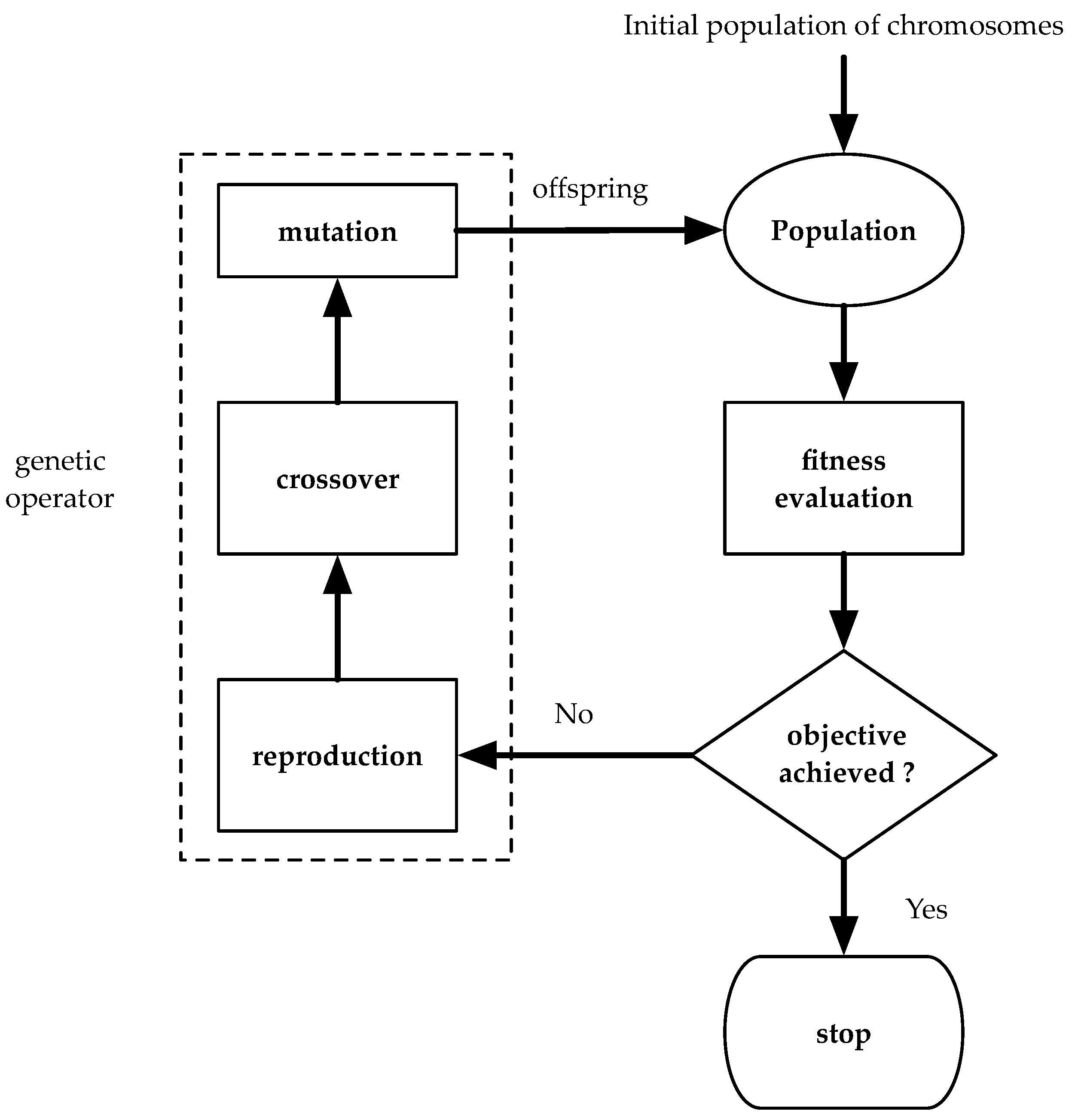
264]). The steps of genetic algorithm are shown in
Figure 19.
The operational modus operandi of GAs involves the generation of a potential solutions population, often depicted as binary genetic code strings. Each solution undergoes an evaluation based on a fitness function gauging its performance. The “fittest” solutions interbreed, producing offspring with inherited traits. The population evolves over iterations, enhancing solution quality. The algorithm is listed in Algorithm 1.
| Algorithm 1. Pseudo code for the genetic algorithm |
| Input: |
| p: population size |
| i: number of individuals in the population |
| v: chromosome |
| x: variable to be solved |
| fit(x): fitness function |
| g, gmax: generation, maximum generation |
| Pc: crossover probability |
| Pm: mutation probability |
| Output: |
| y: solution |
| 1: | encode genes x as chromosomes vi (i = 1, 2 …, p) |
| 2: | initialize the population |
| 2: | while (g < gmax) |
| 1: | calculate individual fitness values fit(xi) |
| 2: | selection |
| 3: | reproduction |
| 3: | crossover |
| 4: | mutation |
| 5: | decoding genes |
| 8: | end while |
| 8: | return x and f(x) |
In the realm of process optimization, each population solution corresponds to unique process parameters, with the fitness function representing the targeted optimization objective (like yield maximization or cost minimization). Across various industries, optimization often necessitates adjustments in three principal parameters: equipment, control, and operation.
Table 12 elucidates these parameters within distinct sectors.
In smart manufacturing, GAs facilitates the optimization of several production facets, including scheduling, routing, and resource allocation. Employing GAs empowers manufacturers to expedite product development cycles, pare down costs, amplify production efficiency, and bolster product quality.
Table 13 offers insights into achieving these objectives across diverse industries and systems.


