Discrete Element Simulations of Contact Heat Transfer on a Batch-Operated Single Floor of a Multiple Hearth Furnace

Abstract

The multiple hearth furnace is a common industrial reactor for the thermal treatment of particulate material. The present contribution concentrates on a numerical analysis of contact heat transfer on a batch-operated single floor of a multiple hearth furnace employing the Discrete Element Method (DEM). The particles are agitated on an electrically heated circular floor by a single rotating rabble arm equipped with three flat blades. Blade angles have been varied from 0° to 90°. The DEM simulations (particle mechanics and contact heat transfer) were validated against experimental data. The transient heating of 20 mm diameter polyoxymethylene (POM) spheres was analysed. As the simulations did not consider natural convection inherently leading to time-varying heat losses, an averaged heat loss parameter was determined to represent heat dissipation from the particles to the surrounding gas and incorporated into the DEM simulations. With this approach, a good agreement with measurements was obtained. The DEM simulations and experiments do not show a large influence of the blade angle on the temporal evolution of the mean particle temperatures. However, the frequency distribution of particle temperature is dependent on the blade angle, revealing an increase in the standard deviation of the frequency distribution with an increasing blade angle.

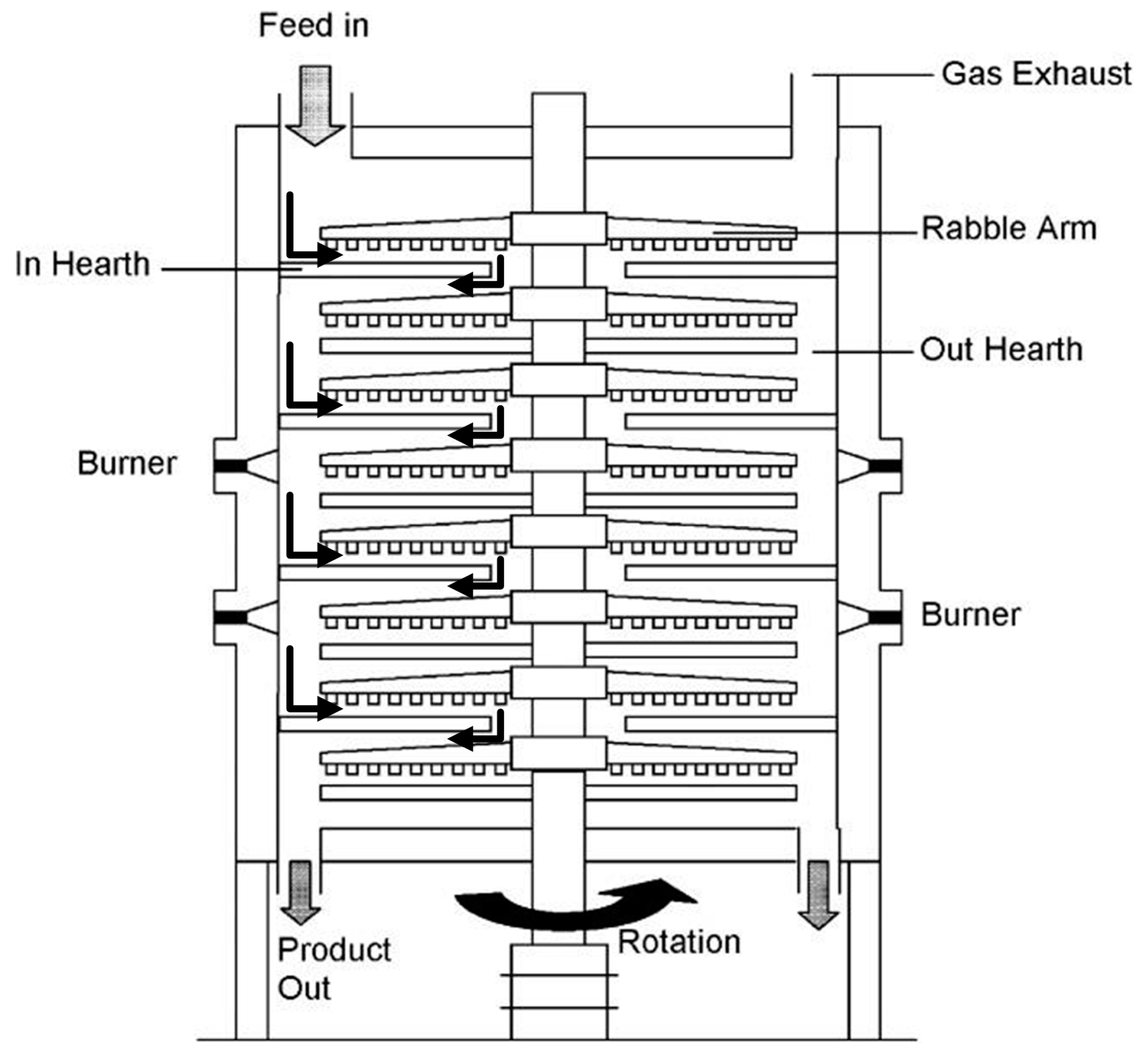
1. Introduction

Typical applications of multiple hearth furnaces are the calcination of minerals [1], the thermal treatment of ores [2], biomass torrefaction [3], or vacuum drying [4]. A sketch of a multiple hearth furnace [1] is depicted in Figure 1. It consists of circular non-moving floors, stacked one above the other. A central rotating shaft is equipped with rabble arms (typically one to four). Blades are attached to the rabble arms that agitate the particle bed.

Particles are fed from the top into the reactor. From there, the particles move through mechanical stirring towards a central opening on the first floor and fall to the next lower level. On the second floor, they are transported from the floor centre to the periphery, where they fall to the subsequent floor; afterwards the process is repeated. Heat for thermal treatment is often provided by radially installed burners. For drying of particles, the required temperature level is typically low, i.e., the high temperatures of a flame could even harm the product properties of the particles to be treated. Therefore, heating of the particles mainly occurs via contact with an internally steam-heated floor at appropriate temperatures for drying [4]. As the goal is uniform product quality, each particle should experience similar thermal boundary conditions over time. Therefore, the particle layer height is typically limited to one to three layers to minimize thermal resistance. This differentiates this application from blade mixers such as presented in [5].

The stirring blades mentioned above are inclined by an angle β against the tangential direction (see Figure 2, [6]). The blade angle β, blade length L, blade thickness B, blade spacing distance s, and particle diameter d_P are the main parameters influencing particle mechanics on the furnace floor. The combination of these parameters results in a particle-free space on the floor that occurs in parallel with a pile-up of particles (heap formation) upstream of the moving blades and a residence time distribution on floors with charge and discharge.

Surprisingly, despite their industrial importance, the number of studies on multiple hearth furnaces is extremely scarce, and most of them concentrate on system aspects. Examples are the work of a group at Aalto University, Finland, who derived a 1D dynamic process model for kaolin calcination in multiple hearth furnaces [3] and derived control strategies based on this dynamic process model [7,8]. A further example of this kind of study is the work of Guatame-Garcia and Buxton [9] presenting a framework for monitoring and quality control of kaolin production.

None of these studies considers the details of particle mechanics on the furnace floor, which, however, are important for an elaborated analysis of contact heat transfer between furnace floor and particles. Some qualitative recommendations concerning blade angle and blade spacing are given in [10] but without any experimental verification. A first study on particle mechanics on a single batch-operated furnace floor was recently presented by the authors’ group [6]. It concentrated on the experimental analysis of particle mechanics of POM spheres with diameters of 5, 10, and 20 mm, respectively. The major findings were that the particle-free surface area increases with stronger inclination of the blades in a radial direction (larger blade angles). The reason for this is the shrinking passage between the blades with a larger blade angle, leading to an increase in the particle-free area behind (downstream) of the blades. Typical maximum values for the particle-free surface areas were in the order of 26 to 31%, depending on particle size. This investigation also showed that the ratio of blade diameter to particle diameter is important for the formation of particle-free areas downstream of the blades at small blade angles, especially when the ratio of blade diameter to particle diameter is large. The present study extends these findings and includes the effect of contact heat transfer.

The numerical simulations in the present study are carried out using DEM. DEM tracks the movement of each individual particle and its interaction with neighbouring particles as well as surrounding walls. With an appropriate thermal model for the calculation of heat transfer, this allows examination of the influence of particle contacts on temperature evolution.

A recent review on heat transfer models for DEM, including radiative heat transfer, convection, and contact heat transfer has been presented by Peng et al. [11]. Contact heat transfer between the particles is described using particle–particle or particle–wall heat transfer coefficients α_PP and α_PW, respectively. Different contact heat transfer models can be found in the literature. They mainly differ in the assumption regarding which effect dominates contact heat transfer: the direct contact of particle (and walls), the gas layer in the vicinity of the contact between particle (and walls), or a combination of both. A thorough discussion on these models can be found in Tsotsas [12].

The simplest model assumes that particle–particle/wall heat transfer takes place only through the direct contact area between particles (or walls) in contact. This model has been introduced by Batchelor and O’Brien [13]. In DEM simulations, the contact area is usually described based on the Hertz theory of contacting spheres [14]. An extension of this model considers varying contact areas with respect to collision time, which has been suggested by Sun and Chen [15] based on the analytical equation for unidirectional, transient heat conduction.

The contribution of Shi et al. [16] on thermal DEM in rotary kilns led to the conclusion that particle–fluid–particle conduction dominates the heat transfer for particles with low thermal conductivity, whereas solid–solid conduction becomes dominant at high particle conductivity. The limiting case that particle–fluid–particle heat transfer dominates can be described using the well-known model of Schlünder [17]. In this model, the modified mean free path of the gas molecules [18] and the width of the gas gap between particle and wall are taken into account. This model has been implemented in DEM by Weigler [19]. From there on, various models for the revised calculation of gas conduction around the contact region have been proposed [20,21].

Tsotsas concluded [12] that both gas and solid phases must be considered. Such a model has been presented by Vargas and McCarthy [22]. Further combinations of models, like in Hou et al. [23], have been presented by splitting the time into short collision and long contact time. During the short collision time, the Sun and Chen [15] model for collision has been combined with the Batchelor and O’Brien contact model in [13]. For longer contact times, approaches based on effective thermal conductivity as the particle–fluid–particle conduction model by Cheng et al. [24] have been proposed.

In this study, spherical, thermally thick particles made from POM are arranged in a single layer on a batch-operated single hearth furnace floor, and the particles are agitated by the rabble arm. Particles with a diameter of 20 mm are used. The surface temperatures during heating of the particles are captured with an infrared camera and compared with DEM simulations.

The research questions addressed are: Can a generalized heat loss parameter that accounts for the heat losses due to natural convection be derived and applied in DEM? Does it deliver correct results without the need of costly DEM/CFD simulations? What is the influence of blade angle on the mean particle temperature and the particle temperature statistics expressed by the frequency distribution? How important is particle–particle heat transfer in comparison to particle–floor heat transfer? What is the ratio of heat transfer through the solid–solid contact to the heat transfer through the gas layer in the vicinity of the contact point?

The core novelty of the present work is given by the fact that—to the best knowledge of the authors—it is the first study in the literature on contact heat transfer on hearth furnace floors, a reactor of high industrial relevance.

2. Discrete Element Method and Contact Heat Transfer Model

2.1. DEM

The simulations are based on an in-house DEM code. In combination with OpenFoam, it has been used, e.g., for the simulation of an oxyfuel operated lime shaft kiln [25].

In the DEM code, the equations for translational and rotational motion are solved numerically using a Euler–Cromer algorithm. The equations read as:

$$m_i\frac{d^2{\overrightarrow{x}}_i}{d{t}^2}=\sum _{j=1}^N{\overrightarrow{F}}_{ij}+m_i\overrightarrow{g},$$

(1)

$${\theta }_i\frac{d^2{\overrightarrow{\phi }}_i}{d{t}^2}=\sum _{j=1}^N{\overrightarrow{M}}_{ij}= \sum _{j=1}^N\left({\overrightarrow{r}}_i\times {\overrightarrow{F}}_{ij}+{\overrightarrow{M}}_j^r\right).$$

(2)

The mass of the particle $i$ is denoted by $m_i$, and its moment of inertia is ${\theta }_i$. The linear acceleration is given by $d^2{\overrightarrow{x}}_i/{dt}^2$, and the angular acceleration of the particle is $d^2{\overrightarrow{\phi }}_i/{dt}^2$. ${\overrightarrow{F}}_{ij}$ and ${\overrightarrow{M}}_{ij}$ are the external force and momentum induced by other particles or walls, while the rolling friction torque is represented by ${\overrightarrow{M}}_j^r$. The distance from the centre of gravity to the contact point of particle/particle or particle/wall is represented by ${\overrightarrow{r}}_i$.

The models used for the calculation of contact forces and torques, together with the values for their parametrization, are given in Appendix A.

2.2. Contact Heat Transfer Model

In the present study, the contact heat transfer model of Vargas and McCarthy [22,26] is used as it considers both direct solid-contact heat transfer and heat transfer through the gas layer between particles, and it showed, e.g., good agreement with measurements in a previous work on a rotating drum [27]. Additionally, the model has been frequently used in recent studies such as the examination of spherical-particle packed beds by the group of Beaulieu [28] and bladed mixers by Hartmanshenn et al. [29]. In the model, the heat transferred between two particles is calculated using the sum of the contact conductivity $H_{\mathrm{c}}$ through direct particle contact and the thermal conductivity $H_{\mathrm{g}}$ through the gas phase, multiplied by the temperature difference $∆T$:

$$\dot{Q}={(H}_{\mathrm{c}}+H_{\mathrm{g}}) ∆T$$

(3)

According to Hertz [30], the contact conductivity $H_{\mathrm{c}}$ can be determined from the harmonic mean of the thermal conductivity ${\lambda }_{\mathrm{h}\mathrm{a}\mathrm{r}\mathrm{m}}$ and the contact radius $a_{\mathrm{c}}$:

$$H_{\mathrm{c}}=2{ \lambda }_{\mathrm{h}\mathrm{a}\mathrm{r}\mathrm{m}}·{ a}_{\mathrm{c}},$$

(4)

$$a_{\mathrm{c}}={\left(\frac{3·\left(1-{\vartheta }^2\right)·{\overrightarrow{F}}^{\mathrm{n}}·r_{\mathrm{e}\mathrm{f}\mathrm{f}}}{2E_{\mathrm{e}\mathrm{f}\mathrm{f}}}\right)}^{\frac{1}{3}}$$

(5)

where $\vartheta$ is the Poisson’s ratio, $E_{\mathrm{e}\mathrm{f}\mathrm{f}}$ is the effective Young’s modulus, $r_{\mathrm{e}\mathrm{f}\mathrm{f}}$ the effective radius, and ${\overrightarrow{F}}^{\mathrm{n}}$ the normal force determined by the spring-damper model (compare Appendix A):

$$E_{\mathrm{e}\mathrm{f}\mathrm{f}}=\frac{2E_i{E}_j}{E_i+E_j}$$

(6)

$$r_{\mathrm{e}\mathrm{f}\mathrm{f}}=\frac{2r_i{r}_j}{r_i+r_j}$$

(7)

$${\lambda }_{\mathrm{e}\mathrm{f}\mathrm{f}}=\frac{2{\lambda }_i{\lambda }_j}{{\lambda }_i+{\lambda }_j}$$

(8)

The thermal conductivity $H_{\mathrm{g}}$ is calculated as the reciprocal of the thermal resistance with the area exposed to the gas $A_{\mathrm{g}}$, the thermal conductivity of the gas ${\lambda }_{\mathrm{g}}$, and the averaged length $l_{\mathrm{g}}$ over which the heat flux applies:

$$H_{\mathrm{g}}=\frac{{\lambda }_{\mathrm{g}}{A}_{\mathrm{g}}}{l_{\mathrm{g}}}$$

(9)

$$A_{\mathrm{g}}=2\pi r^2\left[1-\frac{1}{2}{\left(\frac{a_{\mathrm{c}}}{r}\right)}^2\right]$$

(10)

$$l_{\mathrm{g}}=\frac{r^2\left[1-\frac{\pi }{4}\right]}{r-a_{\mathrm{c}}}$$

(11)

In the current study, the intra-particle heat transport is calculated using a radial shell model dividing each particle into 10 shells with a thickness of 1 mm each.

The parameters used for the heat transfer model are listed in

Table 1. Heat transfer parameters for DEM simulations.

		POM	Aluminium	Steel	Air
Density	[kg/m3]	1420	2700	7700	-
Heat capacity	[J/(kgK)]	1460	900	466	-
Thermal conductivity	[W/(mK)]	0.292	237	50	0.0262
Young’s modulus	[Pa]	3.2 × 109	7.0 × 1010	2.0 × 1011	-
Poisson’s ratio	[-]	0.44	0.33	0.27	-

. The listed material properties are for POM (particles), aluminium (heated bottom plate of the furnace floor), steel (shaft and blades), and air as the surrounding gas.

Heat transfer due to radiation is neglected, which is possible because of the low temperatures studied here. Heat losses due to natural convection are neglected to reduce computational costs of a DEM/CFD coupling.

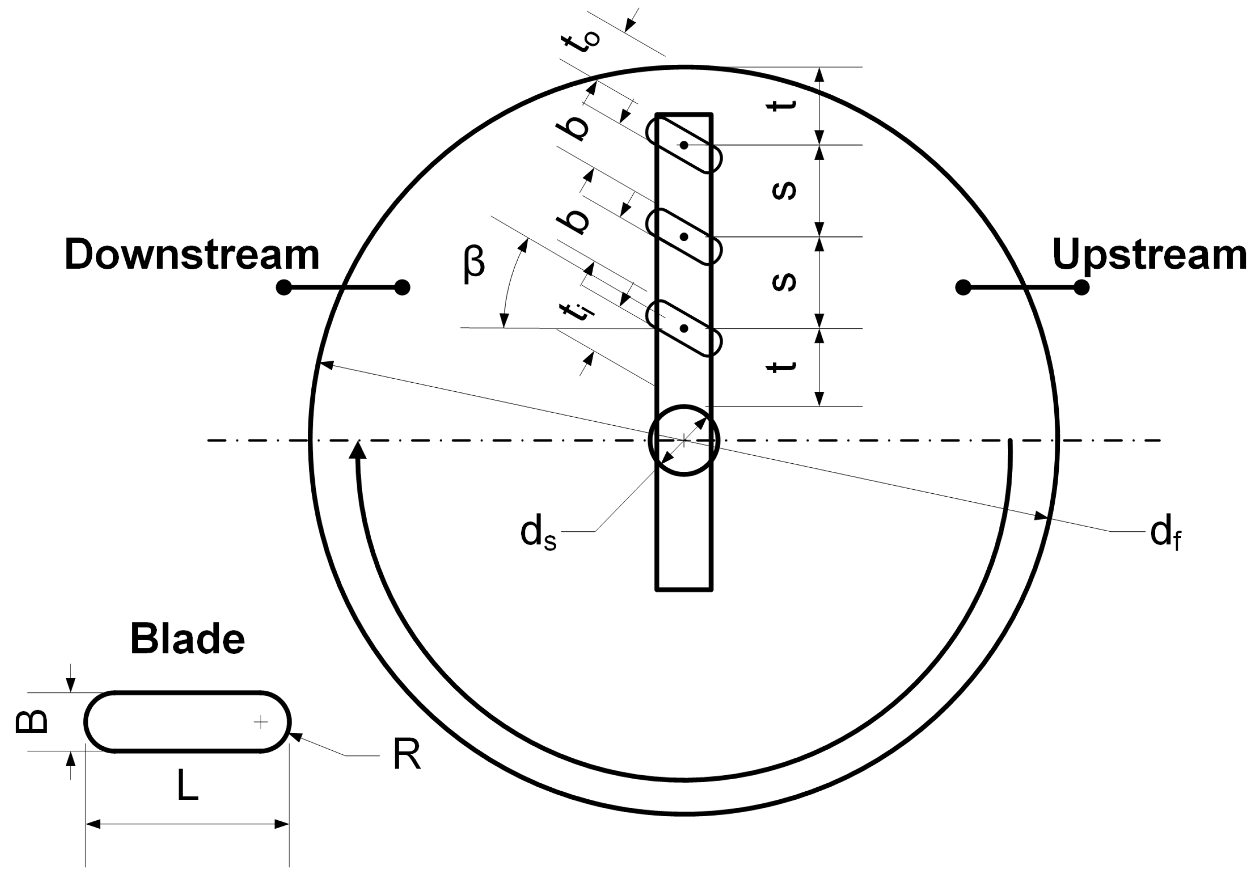
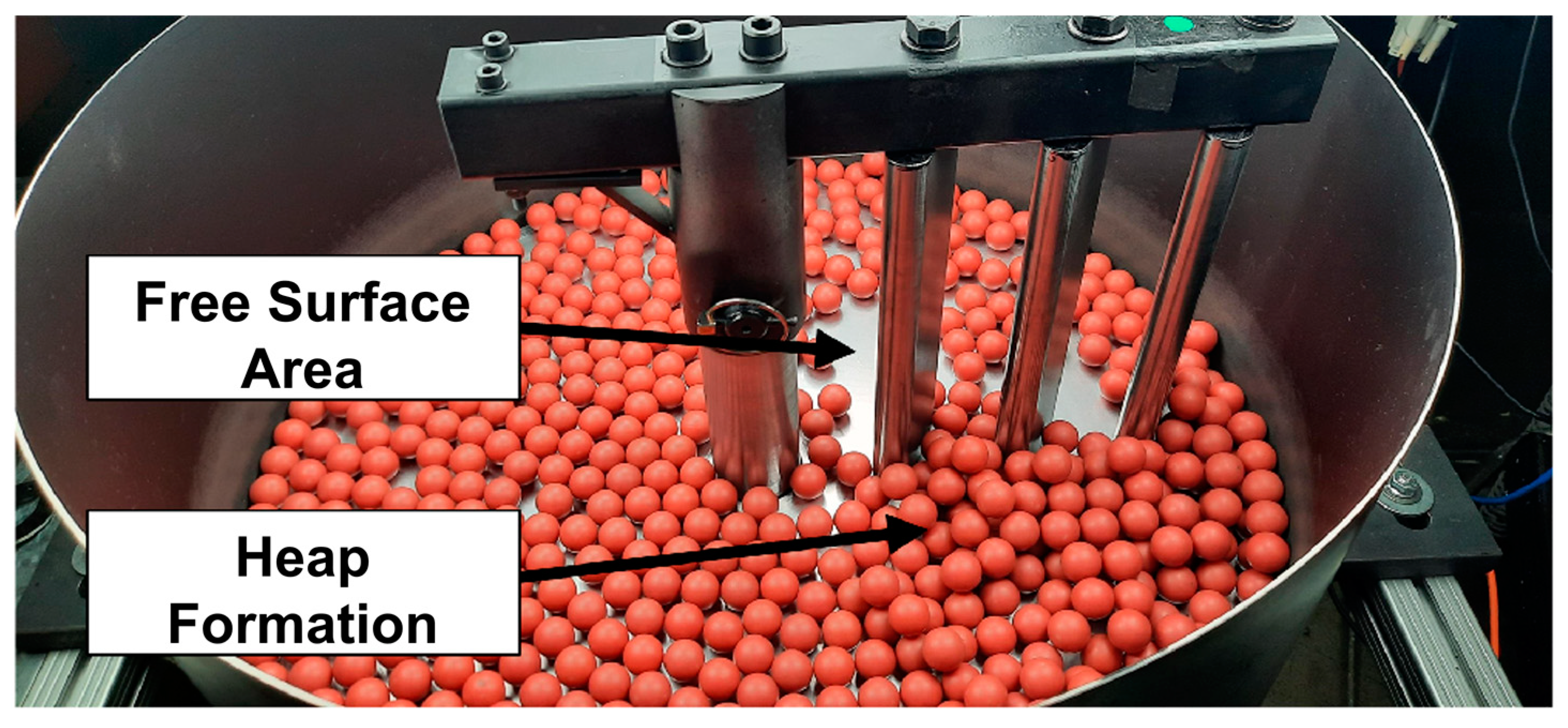
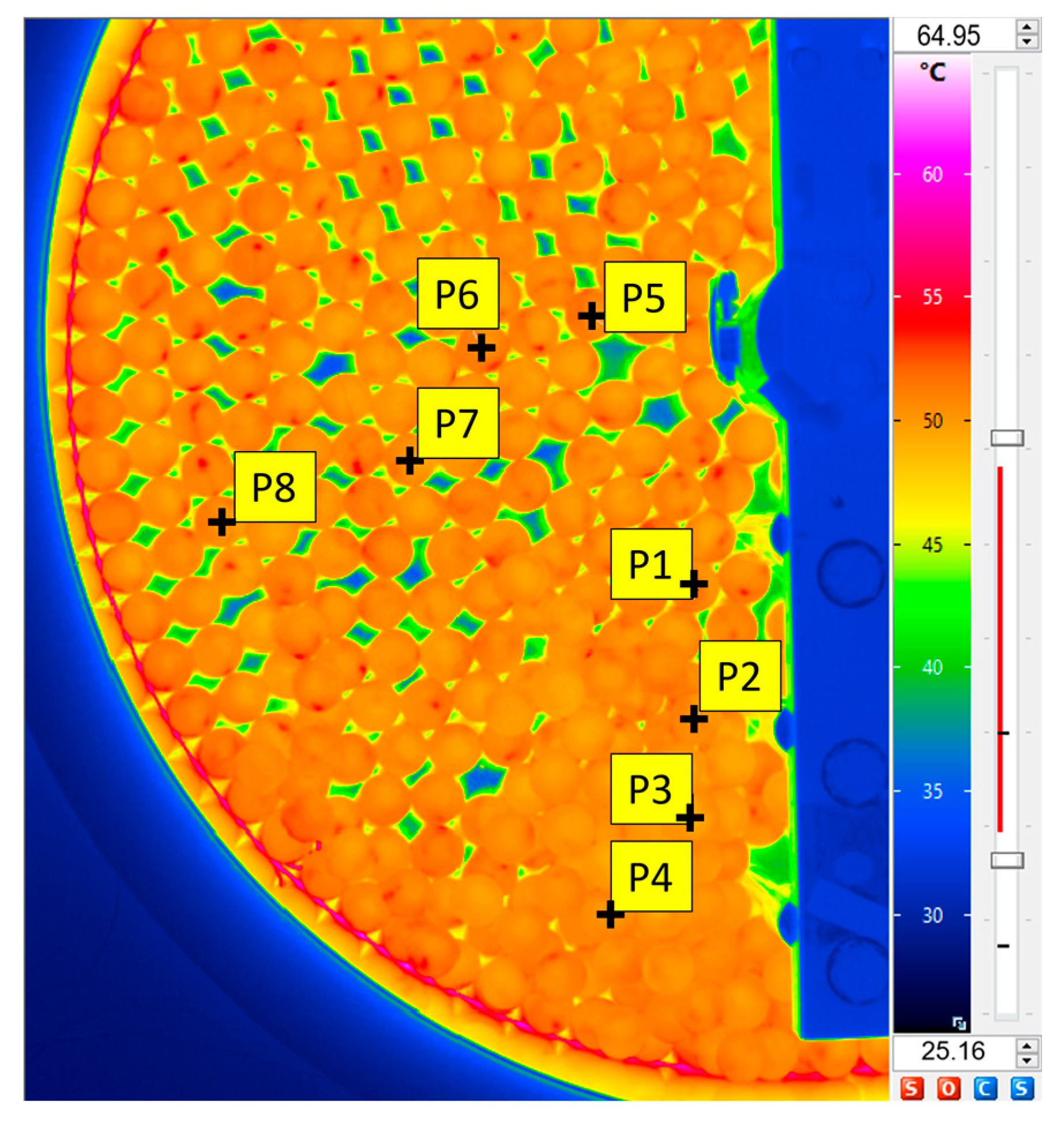
3. Experimental Setup

An existing test rig [6] has been employed for validation of the DEM simulations. All measurements were conducted by the authors’ group in the laboratories at Ruhr University Bochum. A schematic top view of the test rig is depicted in Figure 2. A photograph of the setup can be seen in Figure 3. The circular floor is made of aluminium and has a diameter d_f of 550 mm. The floor is encased by a circular steel blanket. An electric motor actuates the central shaft, which has a diameter d_s of 50 mm and carries three blades on a rabble arm. The blades have a total length L of 60 mm, and the blade ends are hemicylinders with the same radius R as half the blade thickness B (10 mm). The spacing s between the blades is 67.5 mm. The spacing t between blade and central shaft as well as blade and steel blanket is 57.5 mm. The blade angle β can be varied between 0° and 90°.

The passage width b between the blades varies with the blade angle (smaller for larger blade angles). The maximum passage width b is 57.5 mm and corresponds to β = 0°. The minimum passage width b is 7.5 mm and is present at β = 90°. The gaps between blade and steel blanket t_o and blade and shaft t_i also vary with the blade angle. The maximum passage widths t_o and t_i are 52.5 mm and occur at β = 0°. The minimum passage widths for t_a and t_i are 27.5 mm and correspond to β = 90°.

To evaluate the experiments, a digital camera (Basler acA2040-55uc, frame rate 10 fps, image size 2048 × 1536 pixels, purchased from Basler AG, Ahrensburg, Germany) is positioned above the hearth furnace floor. The individual frames from the digital camera are analysed based on a routine programmed in MATLAB R2021a to derive the relative particle-free surface area (RFSA).

The RFSA is determined by dividing the relative visible (not covered by particles) floor surface area (FA) minus the initially visible free surface area (FA₀) before the rabble arm starts to rotate by the overall surface area of the floor (A_fl), RFSA = (FA − FA₀)/A_fl [%].

Furthermore, an infrared camera (InfraTec ImageIR 8380, frame rate 355 fps, image size 640 × 512 pixels, purchased from InfraTec GmbH, Dresden, Germany) is installed above the hearth furnace floor to record particle surface temperatures. Further details of the test rig and data evaluation can be found in [6].

4. Results and Discussion

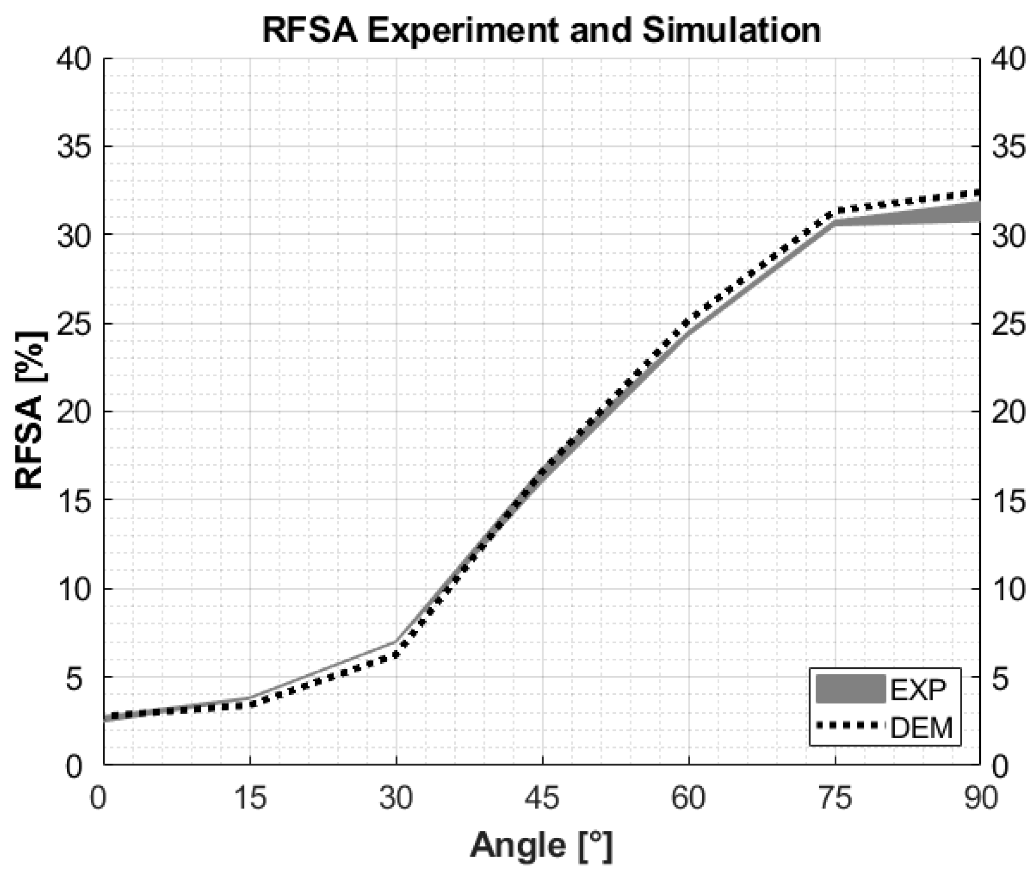
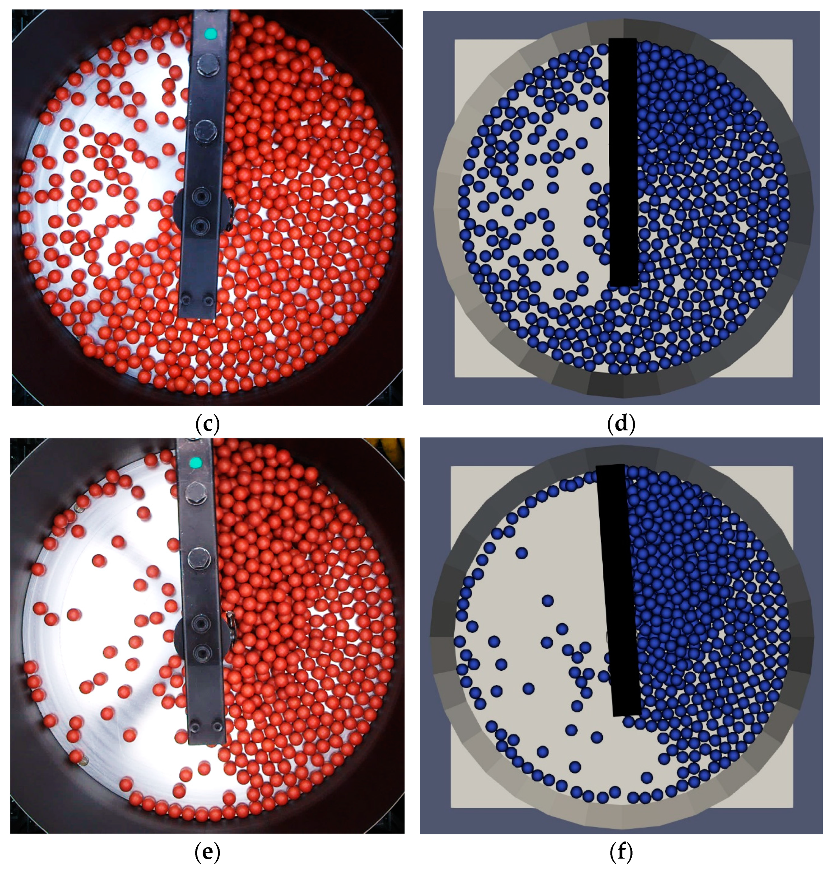
4.1. Validation of Particle Mechanics

As an example, to demonstrate the accuracy of the description of particle mechanics, we present the RFSA results for POM spheres with a diameter of 20 mm from [6]. In the initial state, before shaft rotation, a single layer of particles is present on the floor. The corresponding particle number is 606. The rabble arm rotates at 8 rpm, and the direction of rotation is clockwise. Note that the rotational velocity does not influence the RFSA as centrifugal forces are negligible compared to the forces that the blades impress on the particles, as described in [6], where the kinematics of particle–blade interactions can be found. A centrifugal acceleration event at 8 rpm as in the present test rig is very low and the upper end for industrial applications. Figure 4 presents the experimental and numerical values for the RFSA as a function of blade angle for the steady state, which is reached after 35 revolutions. The grey area represents the deviation between experimental runs, which were repeated three times. The numerical results are displayed using the black dashed line. As expected, less area is covered by particles for larger blade angles, which leads to a correspondingly stronger heap formation in front of the blades. The agreement between simulations and experiments is very good.

In addition, Figure 5 shows a top view of the particle arrangement for 0°, 45°, and 90° blade angles when steady state is reached; the left side depicts an experimental situation, and the right side a numerical simulation. Particle arrangement is very similar, and heap formation upstream of the blades is clearly visible.

The DEM simulations conducted for this study do not include gas-phase movement, i.e., they are not coupled with a CFD solver. Although this is feasible, it would require significant computational effort, especially for the low gas velocity expected due to natural convection above the particle bed. As a consequence of neglecting gas-phase movement, heat losses from convection are not included in the DEM simulation. To account for these losses, a heat loss parameter is determined based on the experiments. This heat loss parameter can then be employed in the DEM simulations to reproduce the experimental results. The procedure of how these heat loss parameters have been derived is described in the following section.

As a first step, the heating of the initially cold particles on the hot hearth furnace floor is examined experimentally. Therefore, the bottom plate of the test rig is heated to 343.15 K. When the target temperature is reached, a single layer of 606 POM spheres (20 mm diameter) is placed on the plate. The time needed for placement of the particles (<20 s) is much smaller than heat-up time scales. The movement of the rabble arm starts immediately after particle placement with a speed of 8 rpm. The experiments are recorded from the top view using an infrared camera with a framerate of two frames per second. The emissivity $\epsilon$ of the POM spheres required to evaluate the thermographic images was determined in [31] and is applied here with a value of 0.95. To obtain comparable measurement data, the areal section observed using the IR camera is always the same. The time of measurement is selected such that the rabble arm is in a similar position in each evaluated image. For each image, eight measuring points are set; four are located upstream of the blades, and the other four are located 45° in front of the blades. The locations P1 to P8 can be seen in Figure 6.

In addition, the temperature of the unheated parts (blades, surrounding walls, and shaft) is measured using thermocouples of type T, with an accuracy of ±0.5 K. The data do not vary with blade angle. The outer wall of the hearth furnace DEM model has been divided in four different temperature zones, representing decreasing temperatures with increasing height difference in regard to the heated plate (see Figure 7). The applied temperatures of the unheated components derived from the measurements are shown in Figure 7.

To assess the importance of the convective heat losses, experimental results for three selected blade angles (Figure 8) are compared to the so-called quasi-adiabatic simulations (Figure 9). The quasi-adiabatic simulations consider heat transfer via contact from the particles to the non-heated parts of the rig. The measured temperatures of the unheated parts are set as boundary conditions in the simulations. As stated earlier, heat losses due to natural convection and radiation have been neglected. Regarding radiation, this is possible because of the low temperatures studied here.

Figure 8 shows the experimentally derived surface temperatures of the particles for three different blade angles. The chosen blade angles represent the minimum impact on the particle bulk (0°), an intermediate impact on the bulk (45°), and the maximum impact (90°). The measured evolution of the temperature for the three blade angles is very similar, and the maximum deviation is approximately one Kelvin.

The corresponding quasi-adiabatic DEM simulations are plotted in Figure 9. The temperatures are the average temperatures of all particles taken from the outermost radial particle shell, representing the particle surface temperature. In contrast to the experiments, the quasi-adiabatic simulations show a clear trend that the heating rates decrease with increasing blade angle. The increase in the blade angle results in an increased heap formation upstream of the blades. This reduces the number of direct particle–floor contacts, leading to smaller heating rates. In addition, the maximum temperature reached after 100 min is lower for larger blade angles. The increased accumulation of the particles upstream of the blades (for larger blade angles) leads to an increase in the particle contacts with non-heated test rig components. This increases the amount of heat flux dissipated. In comparison with the experimental results shown in Figure 8, one can see that the final temperatures reached are in the range of the bottom plate temperature, i.e., 343.15 K, and exceed the experimental results by about 15 K.

To reproduce the experimental temperature evolution, the inclusion of a heat loss parameter in the DEM simulations is required. It is assumed that the heat loss directly depends on the surface of the particle bulk exposed to the surroundings. As a simplification, the same heat loss parameter is applied to each of the particles independent from its location in the bulk. This procedure was adapted from Fischer et al. [32], who examined particle–particle contact heat transfer models in thermal DEM with 10 mm POM and aluminium spheres. The resulting net heat flux ${\dot{Q}}_{\mathrm{P}}$ for a single particle, therefore, is calculated from:

$${\dot{Q}}_{\mathrm{P}}={(H}_{\mathrm{c}}+H_{\mathrm{g}}) ∆T-\alpha A_i·{(T}_{\mathrm{P}}-T_{\mathrm{P}0})$$

(12)

where $\alpha A_i$ represents the heat loss parameter for blade angle $i$, $T_{\mathrm{P}}$ represents the actual particle surface temperature, and $T_{\mathrm{P}0}$ the temperature of the surrounding air, which was set to 298.15 K.

The approach made to determine the heat loss parameter reads as follows:

$$\alpha A_i=\alpha A_0-\left[1-\left(10\ast \frac{T_0-T_i}{T_0}\right)\right]\ast RSF{A}_i,$$

(13)

where $\alpha A_0$ is the initial heat loss parameter for blade angle 0°. $T_0$ represents the final temperature of the particles in the quasi-adiabatic 0° blade angle simulation in [°C], which is equal to the temperature of the heated floor. The final quasi-adiabatic particle temperature at blade angle simulation $i$ is denoted by $T_i$, and the respective particle-free surface area is denoted as $RSF{A}_i$. The final quasi-adiabatic particle temperatures and the $RSF{A}_i$ can be found in Appendix B.

The rationale behind the formulation of the heat loss parameter is as follows. First, it must depend on the particle-free surface area; the larger the RFSA, the stronger the heap formation is, i.e., the particle surface area exposed to the surroundings, and, hence, the heat loss decreases. Second, as reference point for the heat loss parameter, the simulation of the 0° blade angle is used, which shows the maximum convective heat losses as the maximum particle bulk surface area exposed to the surroundings (no heap formation). The specific heat loss parameter $\alpha A_0$ for the 0° blade angle experiments in this case results in 4.04 W/K. The derived heat loss parameters for all blade angles examined are listed in

Table 2. Heat loss parameters [W/K] for blade angles 0°–90°.

$\mathit{\alpha }{\mathit{A}}_0$	$\mathit{\alpha }{\mathit{A}}_{15}$	$\mathit{\alpha }{\mathit{A}}_{30}$	$\mathit{\alpha }{\mathit{A}}_{45}$	$\mathit{\alpha }{\mathit{A}}_{60}$	$\mathit{\alpha }{\mathit{A}}_{75}$	$\mathit{\alpha }{\mathit{A}}_{90}$
4.04	3.69	3.52	2.66	2.07	1.77	1.77

.

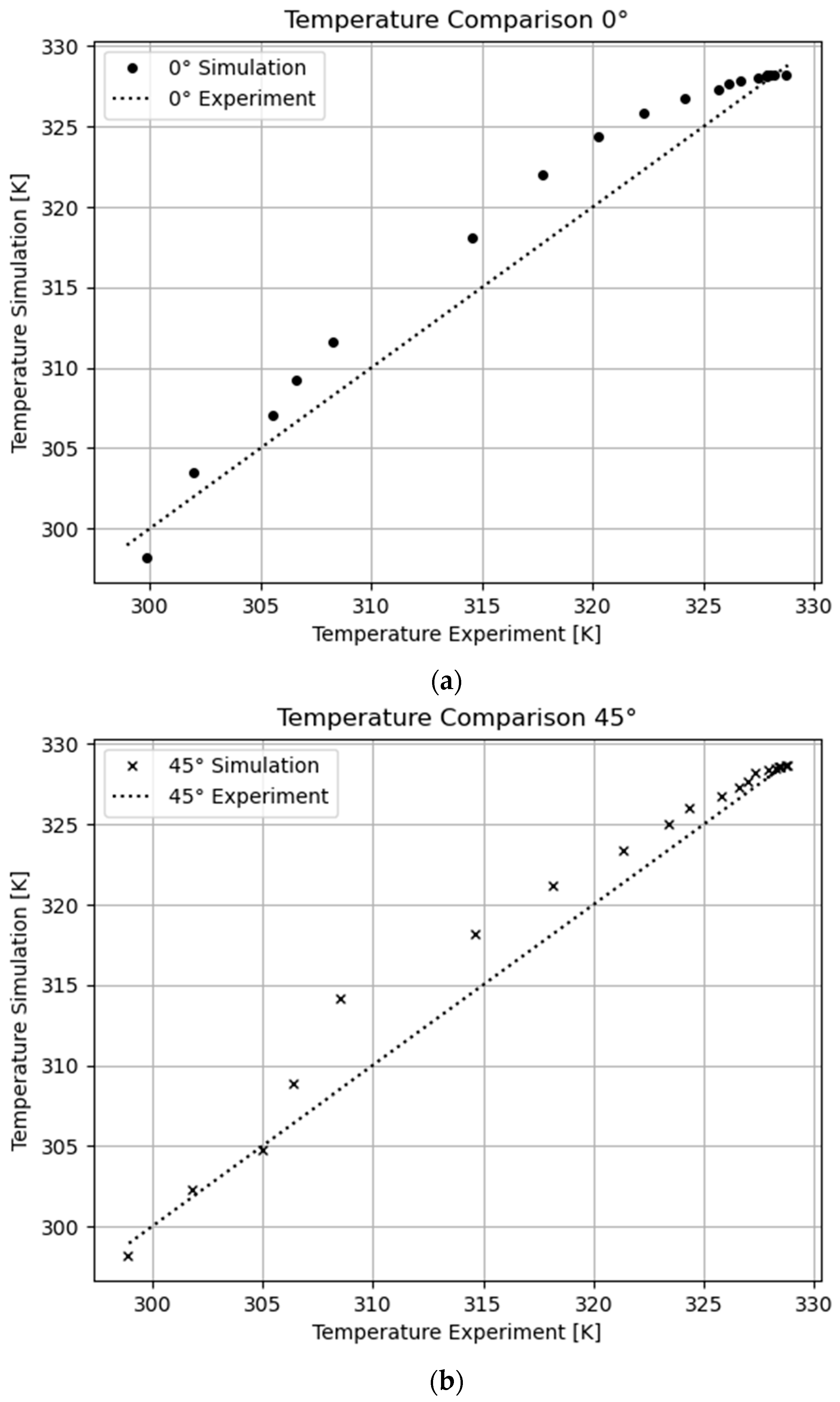
4.2. Numerical Results after Correction for Heat Loss

The above-mentioned heat loss parameters have been implemented in the DEM code. To compare the results, the simulated temperatures (y-axis) are plotted over their corresponding experimental temperatures (x-axis) in Figure 10a–c.

A perfect match would result in the dashed line being inclined by 45°. The lowest temperatures in the diagrams (lower left corner) represent the start of the experiments while the highest temperature (upper right corner) indicates the terminal temperature reached at steady state (after 100 min). Figure 10a–c show that experiments and simulations applying the heat loss parameter are in reasonable agreement. For a 0° blade angle (Figure 10a), the measured terminal temperature is well matched by the simulations with a deviation of 0.5 K. On the other hand, the heating rate of the particles is slightly overestimated, indicated by the fact that the simulated temperatures lie above the 45° line. The maximum deviation between experiments and simulations for the 0° blade angle is 4.3 K (317.73 K experiment/322.0 K simulation). These differences result from the different evaluation methods of the experiment and the simulation. The agitation of the particle bulk using a 0° blade is low. Therefore, the particles have a high temperature gradient between the side of the surface facing the heated plate and the side facing the opposite direction, the IR camera. Therefore, the IR measurement will only detect the cooler side of the particles. In the simulations, the temperature of the outermost particle shell is independent of particle orientation and therefore higher. When reaching the steady-state temperature, the particles in the experiments reach a more homogenised surface temperature due to intra-particle conduction, and the temperature deviations decrease.

The 45° blade angle shows even better agreement (0.05 K deviation) for the measured final temperatures (Figure 10b), but again the heating rate is slightly overpredicted. The data reveal a maximum deviation of 6 K when reaching a 314.19 K simulated temperature while the experimental value is 308.15 K. The differences between the simulation and experiment result here from the accumulation of the bulk upstream of the blades. Since only the optically accessible particle surfaces contribute to the temperature measurement, and the particles that are covered by other particles within the bed are not visible to the infrared camera, the largest particle temperatures are not covered experimentally. It is obvious that the invisible particles in the bottom layers have larger temperatures because they lose less heat to the surrounding gas and are located closer to the heated floor plate. For the evaluation of the simulations, on the other hand, the average temperature of all particles is used, all particles are exposed to the same heat loss parameter at the same time. It can be concluded that potential temperature measurements of the spheres in the lower layers of the accumulated particle bulk would yield higher experimental values and fit the simulations.

Figure 10c displays the results of the 90° blade angle and shows the best agreement for the heating rate, as experiments and simulations follow the straight 45° line. Due to the intense mixing of the bulk, the particles are transported quickly, and the measured temperatures at the optically accessible surface of the bulk represent the most representative mean value. Some minor deviations occur towards the end of the experiments with a deviation 1.2 K for the terminal temperature.

By examining the numerical results in detail, some observations can be made. The comparison of the influence of particle–particle heat transfer to particle–wall heat transfer shows that the heat flux between the particles does not affect the calculated temperatures (Δ < 0.01%). The numerical results of simulations neglecting particle–particle heat transfer prove that for all blade angles solely particle–wall heat transfer drives the temperature increase, and particle–particle heat transfer does not enhance or hinder temperature evolution.

However, striking differences in the temperature curves can be depicted when analysing the heat transfer phenomena of the particle–wall contact itself. The two effects, heat transfer through the direct contact of solids ($H_{\mathrm{c}}$) and heat transfer through the vicinity of the gas layer between particle and wall ($H_{\mathrm{g}}$), are compared in Figure 11. When the heat transfer through the gas layer is neglected, the temperature graph only shows a very slow increase (black solid line). This accompanies the findings of our previous work [32] in which, for thermally thick particles with low heat conductivity, the main heat transport phenomenon takes place through the gas layer. For the present POM material, an analysis of $H_{\mathrm{c}}$ and $H_{\mathrm{g}}$ shows that 99% of the heat is transferred through the gas layer in the vicinity of the contact point.

The grey lines in Figure 11 represent a case in which the material conductivity was raised to a value 1000 times greater than the one for POM (0.292 to 292 W/(mK)). This value is, for example, typical for aluminium. It can be clearly seen that direct contact heat transfer gains importance for these materials (grey solid line). Please note that no other values outside those for conductivity were changed here and that in principle new heat loss parameters must be derived based on measurements.

So far, the average temperatures of all particles have been considered. In the following paragraph, the frequency distributions of the temperatures at different times in the heating process are examined. For this purpose, the frequency distributions of all 606 particles for the angles 0°, 45°, and 90° are shown in Figure 12a–d. In the figures on the top, Figure 12a,b, the temperature distributions for t = 10 and t = 15 min can be seen. The x-axis shows T in [K], and the y-axis shows the frequency density of the particle temperatures. After 10 min simulated time, the distribution for the 0° blade angle shows the smallest standard deviation (${\sigma }_0$ = 1 K), whereas the temperatures in the simulation of the 90° angle show the largest temperature differences (${\sigma }_{90}$ = 2.9 K), where the maximum slightly tends to lower temperatures. The frequency distribution at the 45° blade angle shows two peaks and a standard deviation of ${\sigma }_{45}$ = 2.8 K. The 0° angle shows the most uniform temperatures due to the homogeneous distribution of the spheres on the heated floor and almost no accumulation upstream of the blades. The 45° blade angle simulations show that one of the temperature distribution peaks is located in the same area as the 0° distribution curve. This represents the particles in contact with the heated plate that receive the highest heat flux at this time. The second peak represents the particle accumulation in the upper layers upstream of the blades, which have lower temperatures. Regarding the 90° blade angle, intense accumulation and high particle movement lead to a wide distribution with a peak at the median temperature value.

The evaluation at 15 min simulation time shows similar effects. Overall, temperatures homogenize slightly for all blade angles (${\sigma }_0$ = 0.6 K, ${\sigma }_{45}$ = 2.4 K, and ${\sigma }_{90}$ = 2.7 K). The temperature distribution of the 0° blade angle simulation is further homogenized, while the maximum density values of the 45° and 90° blade angles tend to become larger than the 0° maximum values.

Figure 12c,d show the distribution for 30 and 100 min. Because of the large values for the frequency density at the 0° blade angle, the scaling of the y-axis values has been changed.

The frequency distribution at 30 min shows reduced standard deviation compared to 10 and 15 min for all blade angles (${\sigma }_0$ = 0.2 K, ${\sigma }_{45}$ = 1.4 K, and ${\sigma }_{90}$ = 1.8 K). The results show very similar averaged temperatures for all blade angles here. For the 90° blade angle, the median temperature now reaches the highest density and is nearly the same as the 0° blade angle median temperature. In contrast to the other blade angles, the local minimum of the 45° distribution occurs at the median temperature. The maximum temperatures of 45° and 90° blade angles are about 6 K higher than for the 0° blade angle. These trends continue until the end of the simulation time after 100 min. The calculated temperatures have reached final state here for all blade angles (${\sigma }_0$ = 0.2 K, ${\sigma }_{45}$ = 0.9 K, and ${\sigma }_{90}$ = 1 K).

The results show that the 45° blade angle develops a layering of temperatures, which does not occur for the other blade angles. This is an important observation regarding industrial processes. Such temperature stratification may have a negative effect on the product quality if homogeneity of product properties is to be achieved. The closely spaced temperatures of the 0° blade angle result from the lack of accumulation of the particles. However, due to the low rotation of the particles, it is likely that temperature differences occur inside the particle surface, as the particle surface that is in direct contact with the floor receives heat via conduction, whereas surface areas exposed to the surroundings stay cold.

The 90° blade angle shows the widest spread of temperatures, which is important to know for the setting of certain product properties when specific material temperatures are mandatory.

5. Conclusions and Future Work

In this study, the experimentally observed heating behaviour of an initially cold single layer of 20 mm polyoxymethylene (POM) spheres on a floor of a hearth furnace is compared with the results of Discrete Element Method (DEM) simulations. The particles are thermally thick and are agitated on an electrically heated circular floor by a single rotating rabble arm equipped with three flat blades. The blade angle, defined as the angle that the blades are inclined against the tangential direction, is varied from 0° to 90°.

The contact heat transfer model applied in DEM accounts for the heat transfer through the gas layer in the vicinity of the solid–solid contact point and also for the direct heat transfer through the solid contact point. Radiative heat transfer can safely be neglected due to the low temperatures of the system. To account for convective heat losses via natural convection, but in parallel to avoid costly DEM/CFD simulations, an averaged particle-based heat loss parameter is derived from experiments for every examined blade angle. The parameter is mainly dependent on the relative particle-free surface area (RFSA) on the hearth furnace floor.

Based on the results of experiments and DEM simulations, the following conclusions can be drawn:

• A costly DEM-CFD coupling can be avoided for the present setup. The heat loss parameter derived for DEM allows us to predict the temperature evolution of the particles for all angular positions of the blades in good agreement with the values taken from the experiments.
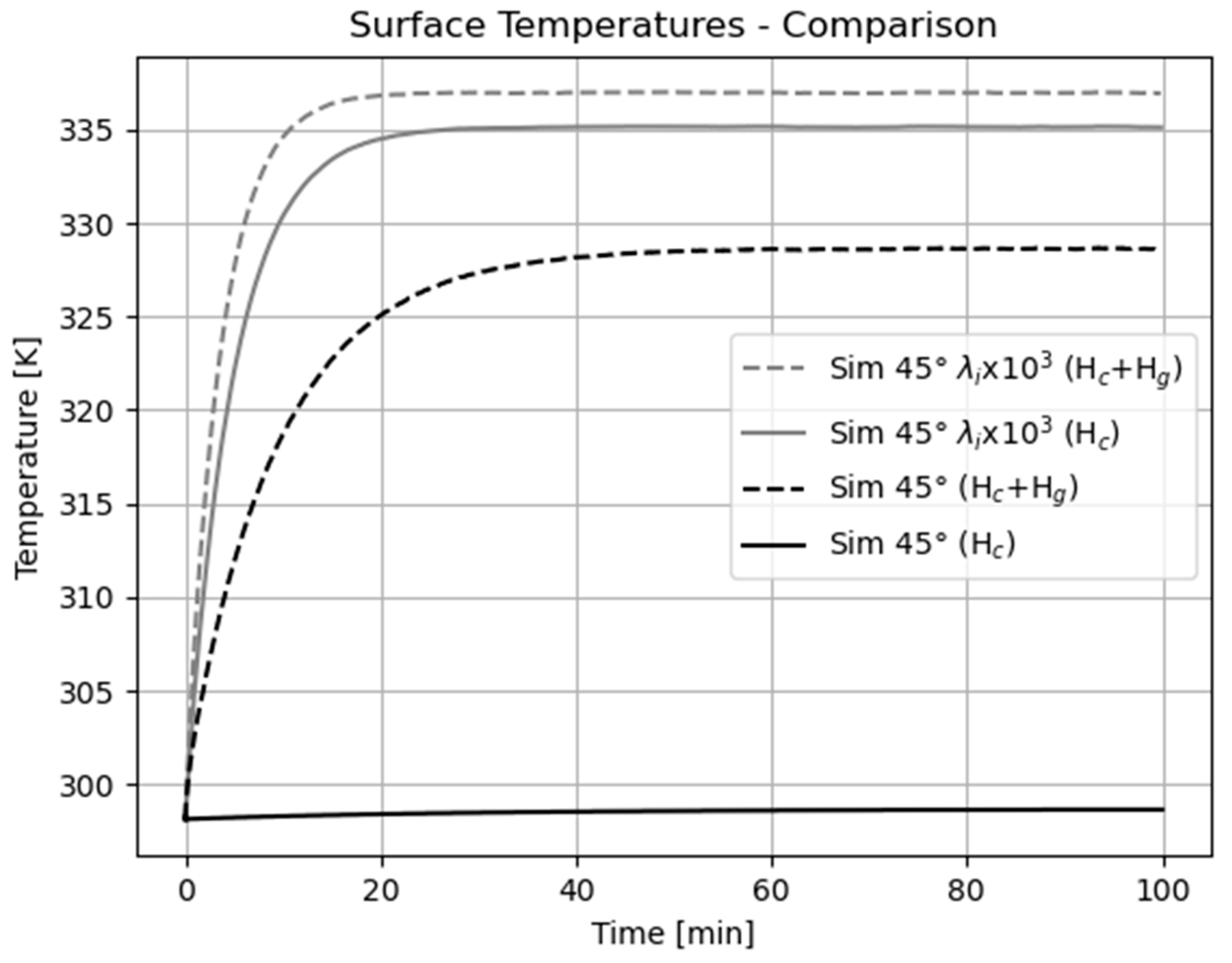
• Particle–floor contact heat transfer clearly dominates over particle–particle heat transfer. Furthermore, it turned out that for low thermal conductivity POM particles, the heat transfer through the gas layer in the vicinity of the contact point of the particles with the floor is much larger than the direct heat transfer through solid–solid contact. This behaviour changes for high thermal conductivity materials such as aluminium, where solid–solid-contact heat transfer cannot be neglected. Changes may also occur at higher temperatures when radiative transport becomes important.
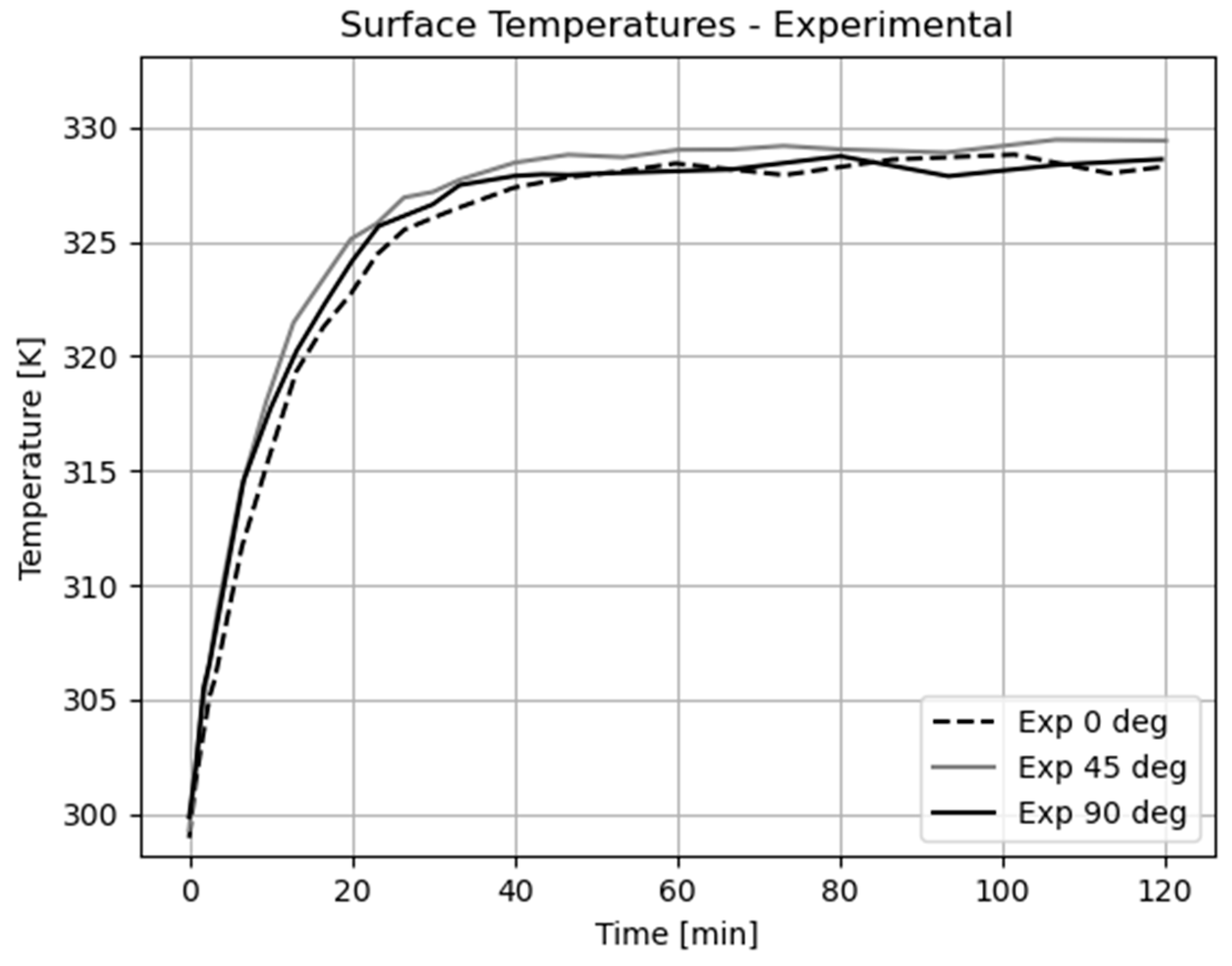
• The blade angle has hardly any influence on the temporal evolution of the particle temperatures. This is due to two opposite effects. As the blade angle increases, the heat transfer from the plate to the spheres is reduced, since the number of spheres in direct contact with the hot floor is smaller. This occurs due to the accumulation of the particles upstream of the blades. This accumulation simultaneously causes the convective heat loss to be reduced, as the surface area of the bulk exposed to the surrounding gas is reduced. These two effects seem to balance each other.
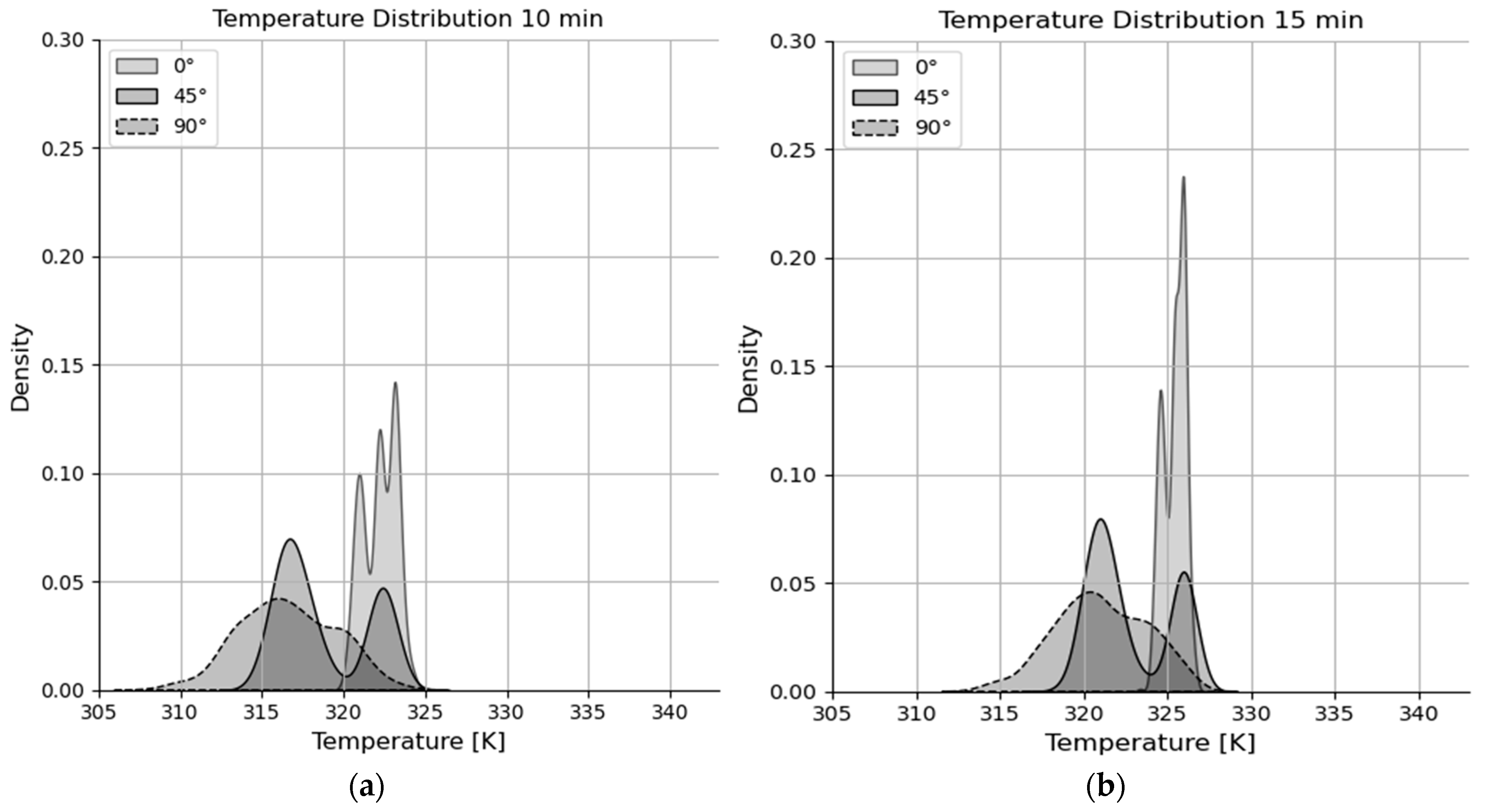
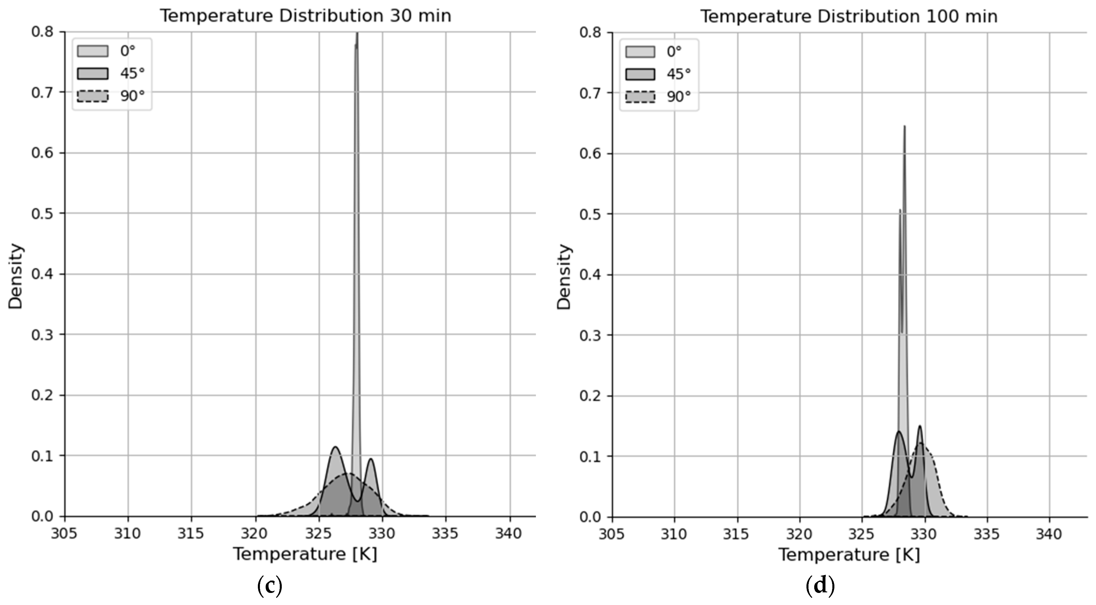
• The frequency distribution of particle temperature depends on the blade angle. The standard deviation increases with the blade angle, and for a 45° blade angle a bimodal frequency distribution develops, whereas for the 0° and 90° blade angles monodisperse frequency distributions prevail.

In particular, finding 4 is of high importance for industrial practice as even small temperature deviations among the particles in the bulk may lead to differing product quality for kinetically controlled product reactions.

The authors are aware that the current study is only a first step towards the understanding of contact heat transfer on hearth furnace floors, and further investigations are needed. Specifically, a 3D model for intra-particle heat transfer would be beneficial as the radial heat conduction model used in the current study cannot resolve the effects observed in the experiments, where particles get locally hot where in contact with the hot floor but stay cold at the opposite side of the particle. A 3D intra-particle heat transfer model would improve the predictive capabilities of the simulations. Furthermore, the thermal behaviour of multilayer bulk assemblies must be studied, and batch operation, as in the present study, must be replaced by experiments with charge and discharge of particles as in industrial practice. In continuous operation, the blade angles will influence particle residence time on the floor, and consequently the evolution of the mean particle temperature will then depend on the blade angle.

References

- Eskelinen, A.; Zakharov, A.; Jämsä-Jounela, S.-L.; Hearle, J. Dynamic modeling of a multiple hearth furnace for kaolin calcination. AIChE J. 2015, 61, 3683–3698. [Google Scholar] [CrossRef]
- Thyssenkrupp: MULTIPOL—Multiple Hearth Furnace. Available online: https://ucpcdn.thyssenkrupp.com/_legacy/UCPthyssenkruppBAIS/assets.files/products___services/mineral_processing/pyroprocessing_systems/product_sheet-multipol-en-webview.pdf (accessed on 11 July 2023).
- Lampe, K.; Grund, G.; Erpelding, R.; Denker, J. Biocoal preparation—Biomass a sustainable fuel for industrial processes. In Proceedings of the 6th European Metallurgical Conference EMC 2011, Aachen, Germany, 26–29 June 2011; Volume 5, pp. 1623–1630. [Google Scholar]
- Liu, X.; Jiang, J. Mass and Heat Transfer in a Continuous Plate Dryer. Dry. Technol. 2004, 22, 1621–1635. [Google Scholar] [CrossRef]
- Siraj, M.S.; Radl, S.; Glasser, B.J.; Khinast, J.G. Effect of blade angle and particle size on powder mixing performance in a rectangular box. Powder Technol. 2011, 211, 100–113. [Google Scholar] [CrossRef]
- Kriegeskorte, M.; Hilse, N.; Spatz, P.; Scherer, V. Experimental study on influence of blade angle and particle size on particle mechanics on a batch-operated single floor of a multiple hearth furnace. Particuology 2023, 85, 224–240. [Google Scholar] [CrossRef]
- Jämsä-Jounela, S.-L.; Gomez Fuentes, J.V.; Hearle, J.; Moseley, D.; Smirnov, A. Control strategy for a multiple hearth furnace in kaolin production. Control Eng. Pract. 2018, 81, 18–27. [Google Scholar] [CrossRef]
- Gomez, F.J.V.; Jämsä-Jounela, S.L. Control Strategy for a Multiple Hearth Furnace. IFAC—PapersOnLine 2018, 51, 189–194. [Google Scholar] [CrossRef]
- Guatame-Garcia, A.; Buxton, M. Framework for Monitoring and Control of the Production of Calcined Kaolin. Minerals 2020, 10, 403. [Google Scholar] [CrossRef]
- Autogenous Roasting of Low-Grade Zinc in Multiple Hearth Furnace at Risdon. Available online: https://www.911metallurgist.com/autogenous-roasting-low-grade-zinc/ (accessed on 11 July 2023).
- Peng, Z.; Doroodchi, E.; Moghtaderi, B. Heat transfer modelling in Discrete Element Method (DEM)-based simulations of thermal processes: Theory and model development. Prog. Energy Combust. Sci. 2020, 79, 100847. [Google Scholar] [CrossRef]
- Tsotsas, E. Particle-particle heat transfer in thermal DEM: Three competing models and a new equation. Int. J. Heat Mass Transf. 2019, 132, 939–943. [Google Scholar] [CrossRef]
- Batchelor, G.K.; O’Brien, R.W. Thermal or electrical conduction through a granular material. Proc. R. Soc. Lond. Ser. A. Math. Phys. Sci. 1977, 355, 313–333. [Google Scholar] [CrossRef]
- Kruggel-Emden, H.; Simsek, E.; Rickelt, S.; Wirtz, S.; Scherer, V. Review and extension of normal force models for the Discrete Element Method. Powder Technol. 2007, 171, 157–173. [Google Scholar] [CrossRef]
- Sun, J.; Chen, M. A theoretical analysis of heat transfer due to particle impact. Int. J. Heat Mass Transf. 1988, 31, 969–975. [Google Scholar] [CrossRef]
- Shi, D.; Vargas, W.L.; McCarthy, J.J. Heat transfer in rotary kilns with interstitial gases. Chem. Eng. Sci. 2008, 63, 4506–4516. [Google Scholar] [CrossRef]
- Schlünder, E.U. Wärmeübergang an bewegte Kugelschüttungen bei kurzfristigem Kontakt. Chem. Ing. Tech. 1971, 43, 651–654. [Google Scholar] [CrossRef]
- Tsotsas, E. M6 Heat Transfer from a Wall to Stagnant and Mechanically Agitated Beds. In VDI Heat Atlas; VDI e. V.: Berlin/Heidelberg, Germany; Springer: Berlin/Heidelberg, Germany, 2010; pp. 1311–1326. [Google Scholar] [CrossRef]
- Weigler, F. Diskrete Untersuchung des Aufheizverhaltens von Partikelschüttungen. Ph.D. Thesis, Otto-von-Guericke-Universität Magdeburg, Magdeburg, Germany, 2012. [Google Scholar] [CrossRef]
- Morris, A.B.; Pannala, S.; Ma, Z.; Hrenya, C.M. A conductive heat transfer model for particle flows over immersed surfaces. Int. J. Heat Mass Transf. 2015, 89, 1277–1289. [Google Scholar] [CrossRef]
- Wang, S.; Luo, K.; Hu, C.; Lin, J.; Fan, J. CFD-DEM simulation of heat transfer in fluidized beds: Model verification, validation, and application. Chem. Eng. Sci. 2019, 197, 280–295. [Google Scholar] [CrossRef]
- Vargas, W.L.; McCarthy, J.J. Heat conduction in granular materials. AIChE J. 2001, 47, 1052–1059. [Google Scholar] [CrossRef]
- Hou, Q.F.; Zhou, Z.Y.; Yu, A.B. Computational study of heat transfer in a bubbling fluidized bed with a horizontal tube. AIChE J. 2012, 58, 1422–1434. [Google Scholar] [CrossRef]
- Cheng, G.J.; Yu, A.B.; Zulli, P. Evaluation of effective thermal conductivity from the structure of a packed bed. Chem. Eng. Sci. 1999, 54, 4199–4209. [Google Scholar] [CrossRef]
- Illana, E.; Merten, H.; Wirtz, S.; Scherer, V. DEM/CFD Simulations of a Generic Oxy-Fuel Kiln for Lime Production. Therm. Sci. Eng. Prog. 2023, 45, 102076. [Google Scholar] [CrossRef]
- Vargas, W.L.; McCarthy, J. Conductivity of granular media with stagnant interstitial fluids via thermal particle dynamics simulation. Int. J. Heat Mass Transf. 2002, 45, 4847–4856. [Google Scholar] [CrossRef]
- Komossa, H.; Wirtz, S.; Scherer, V.; Herz, F.; Specht, E. Heat transfer in indirect heated rotary drums filled with monodisperse spheres: Comparison of experiments with DEM simulations. Powder Technol. 2015, 286, 722–731. [Google Scholar] [CrossRef]
- Beaulieu, C.; Vidal, D.; Yari, B.; Chaouki, J.; Bertrand, F. Impact of surface roughness on heat transfer through spherical particle packed beds. Chem. Eng. Sci. 2021, 231, 116256. [Google Scholar] [CrossRef]
- Hartmanshenn, C.; Chaksmithanont, P.; Leung, C.; Ghare, D.V.; Chakraborty, N.; Patel, S.; Halota, M.; Khinast, J.G.; Papageorgiou, C.D.; Mitchell, C.; et al. Infrared temperature measurements and DEM simulations of heat transfer in a bladed mixer. AIChE J. 2022, 68, e17636. [Google Scholar] [CrossRef]
- Hertz, H. Ueber die Berührung fester elastischer Körper. Crll 1882, 1882, 156–171. [Google Scholar] [CrossRef]
- Rickelt, S. Discrete Element Simulation and Experimental Validation of Conductive and Convective Heat Transfer in Moving Granular Material. In Berichte aus der Energietechnik; Shaker Verlag: Aachen, Germany, 2011. [Google Scholar]
- Fischer, J.; Rodrigues, S.; Kriegeskorte, M.; Hilse, N.; Illana, E.; Scherer, V.; Tsotsas, E. Particle-particle contact heat transfer models in thermal DEM: A model comparison and experimental validation. Powder Technol. 2023, 429, 118909. [Google Scholar] [CrossRef]
- Maxwell, J.C., IV. On the dynamical theory of gases. Philos. Trans. R. Soc. Lond. 1867, 157, 49–88. [Google Scholar] [CrossRef]
- Zhou, Y.C.; Wright, B.D.; Yang, R.Y.; Xu, B.H.; Yu, A.B. Rolling friction in the dynamic simulation of sandpile formation. Phys. A Stat. Mech. Its Appl. 1999, 269, 536–553. [Google Scholar] [CrossRef]