Article

On the Development of Descriptor-Based Machine Learning Models for Thermodynamic Properties: Part 1—From Data Collection to Model Construction: Understanding of the Methods and Their Effects

Université de Lorraine, CNRS, LRGP, F-54001 Nancy, France
*
Author to whom correspondence should be addressed.
Processes 2023, 11(12), 3325; https://doi.org/10.3390/pr11123325
Submission received: 20 October 2023 / Revised: 13 November 2023 / Accepted: 17 November 2023 / Published: 29 November 2023

Abstract

:
In the present work, a multi-angle approach is adopted to develop two ML-QSPR models for the prediction of the enthalpy of formation and the entropy of molecules, in their ideal gas state. The molecules were represented by high-dimensional vectors of structural and physico-chemical characteristics (i.e., descriptors). In this sense, an overview is provided of the possible methods that can be employed at each step of the ML-QSPR procedure (i.e., data preprocessing, dimensionality reduction and model construction) and an attempt is made to increase the understanding of the effects related to a given choice or method on the model performance, interpretability and applicability domain. At the same time, the well-known OECD principles for the validation of (Q)SAR models are also considered and addressed. The employed data set is a good representation of two common problems in ML-QSPR modeling, namely the high-dimensional descriptor-based representation and the high chemical diversity of the molecules. This diversity effectively impacts the subsequent applicability of the developed models to a new molecule. The data set complexity is addressed through customized data preprocessing techniques and genetic algorithms. The former improves the data quality while limiting the loss of information, while the latter allows for the automatic identification of the most important descriptors, in accordance with a physical interpretation. The best performances are obtained with Lasso linear models ( M A E test = 25.2 kJ/mol for the enthalpy and 17.9 J/mol/K for the entropy). Finally, the overall developed procedure is also tested on various enthalpy and entropy related data sets from the literature to check its applicability to other problems and competing performances are obtained, highlighting that different methods and molecular representations can lead to good performances.

1. Introduction

Quantitative Structure Property/Activity Relationship (QSPR/QSAR) models have been widely employed for several decades in chemistry-related fields to predict various endpoints of molecules (i.e., physico-chemical properties and biological activities, respectively) on the basis of their structure (e.g., descriptors, fingerprints, graphs), via mathematical methods. Successful QSPR/QSAR applications include very different endpoints such as critical temperature and pressure [1], normal boiling point [2], heat capacity [3], enthalpy of solvation [4]/vaporization [5,6], blood-brain barrier permeability [7], physico-chemical properties of polymers/fuels/ionic liquids [8,9,10,11,12,13,14,15], solubility [16,17,18,19,20,21], minimum ignition energy of combustible dusts [22] or antibacterial/antiviral properties [23,24].
To construct these QSPR/QSAR models, numerous mathematical methods were used ranging from simple and interpretable linear regression methods (e.g., multiple linear regression and partial least squares) to more complex and nonlinear machine learning (ML) and deep learning methods, in response to the rising complexity of available data sets (e.g., larger data sets, nonlinear relations between molecular structures and endpoints, diversity in the molecular structures) [25,26,27,28,29]. Similarly, significant progress has been made in terms of the molecular structure representation, which evolved from simple representations (e.g., with few descriptors) to more complex ones (e.g., with up to thousands of descriptors, or based on graph neural networks (GNN)). More generally, the need to discover and develop more rapidly new molecules and properties has kept QSPR/QSAR research particularly active. These data-driven models effectively circumvent the complex and time-consuming development of knowledge-based models and experimental studies. More examples of artificial intelligence and ML application in various subfields of chemistry can be found in [30,31].
However, many QSPR/QSAR works lack important elements and fail to properly address the recommendations from the OECD (Organization for Economic Co-operation and Development) [25,32,33]. In particular, these recommendations are composed of 5 principles aiming at ‘facilitating the consideration of a (Q)SAR model for regulatory purposes’, for example when predicting the health hazards and toxicity of new chemicals [25,29]. These principles dictate that any relevant study should clearly include a defined endpoint, an unambiguous algorithm, a defined domain of applicability, appropriate measures of goodness-of-fit/robustness/predictivity and, if possible, a mechanistic interpretation [34]. Even if they were initially established to predict the hazards of chemicals, these general principles well-addressed the critical aspects during the development of any ML procedure. Besides, the use of ML methods has exploded over the last decades and there is a lack of “rules” to control whether the models are properly developed, which would facilitate their use and acceptance. Developing a ML model without possible further application is indeed useless. For all these reasons, the OECD principles were considered in this work in the case of thermodynamic properties.
The development of any ML-QSPR/QSAR model is generally composed of the following well-known steps: data collection, data preprocessing, dimensionality reduction, model construction and applicability domain definition. Along the implementation of these steps, a great number of methods and choices are presented to the developer, depending also on the characteristics of the problem and the available data, and these have a direct impact on the model performance, interpretability and applicability (e.g., to a new chemical). However, a clear overview of the possible methods or a clear justification of a choice over another one does not typically accompany relevant studies, thus making it unclear whether the proposed solution is general or robust enough for the envisioned application area. Accordingly, the first and main contribution of this work is to break-down and analyze the different steps of the development of a ML-QSPR/QSAR model in an attempt to assess the impact and the contribution of each choice and method along the process, while considering the OECD principles. The objective of this methodological approach will be the development of a predictive ML-QSPR model for two thermodynamic properties of molecules, namely the enthalpy of formation and the absolute entropy for the ideal gas state of molecules at 298.15 K and 1 bar. The representation of the molecules will be based on molecular descriptors.
The enthalpy of formation and entropy, which are the endpoints of interest in this study, are crucial to many chemical applications. In particular, they are required in the design of molecules, since they impact molecular stability; they are also present in the development of kinetic models and the prediction of reactions since they influence energy balances and equilibrium. Accordingly, the design of any process, involving chemical reactions or heat transfer, is prone to depend on the existence of accurate models for the prediction of these properties. Among the most common approaches to predict them, quantum chemistry (QC) and group contribution (GC) methods have been largely employed so far for their accuracy (e.g., <1 kcal/mol for the enthalpy of formation of small molecules) and/or simplicity [35,36,37,38,39,40,41,42,43,44]. However, for large/complex molecules, QC methods become physically and computationally complex, while for GC methods, the decomposition of the molecules into known groups becomes a tedious/infeasible task and corrections due to the contribution of the 3D overall structure are needed (e.g., to include steric effects and ring strain effects). Consequently, ML methods represent an interesting alternative to the aforementioned QC and GC approaches due to their accuracy, low computation time and ability to describe complex problems without requiring physical knowledge. At the same time, ML methods, being data-driven in nature, suffer from a lack of interpretability and extrapolability, in comparison to their QC and GC knowledge-based counterparts [45].
Molecular descriptors represent diverse structural and physico-chemical characteristics of the molecules. Thousands of different descriptors have been reported in the literature and their calculation is nowadays facilitated by the use of publicly accessible libraries and software (e.g., RDKit, AlvaDesc, PaDEL, CDK, Mordred) [46,47,48,49,50]. In particular, the software AlvaDesc, which was employed in the present study, generates a total of 5666 descriptors for each molecule. This relatively high number of descriptors (i.e., concerning a physico-chemical problem) contains rich information on the molecular structures and thus increases the chances of capturing the relevant features affecting the thermodynamic properties, in the absence of knowledge. At the same time, this poses a number of difficulties in the development of the ML-QSPR/QSAR model and its generalized implementation and interpretation. These difficulties are related to the need to distinguish, at a certain point within the development procedure, the number and identity of the most relevant descriptors to the endpoints of interest, which remains one of the biggest challenges related to the use of descriptors (a.k.a. the “curse of dimensionality”). Commonly, to overcome these issues, a dimensionality reduction step is implemented before the model construction. On the one hand, feature extraction methods project the original high-dimensional space into a new space of lower dimension, thus creating new features being linear or nonlinear combinations of the original ones. On the other hand, feature selection methods select only a limited subset of descriptors as being the most representative ones and the rest are discarded, which facilitates the interpretability of the subsequent model in comparison with feature extraction methods. The selection of descriptors can also be based on available knowledge (i.e., expert input) but such knowledge is not readily available for the complete list of generated descriptors. These difficulties and the different dimensionality reduction approaches that can be undertaken under the premise that physical knowledge is not available a priori for all 5666 descriptors are analyzed as part of this work. A mechanistic interpretation of the descriptors that are identified as highly relevant by the different approaches is also attempted.
Finally, this study was not constrained to molecules belonging to a limited number of chemical families and structures, but, within the perspective of the discovery of new molecules for various applications, the development of models that will be applicable to a large diversity of molecules was pursued. Note, that this is a specific differentiating point of the present study and a major challenge as many reported studies are restricted to molecules of specific chemical families and/or structural characteristics [51,52,53,54,55,56,57].
More generally, this work constitutes a multi-angle, holistic approach to the procedure for the development of generally-applicable ML-QSPR/QSAR models, based on a high-dimensional representation of molecules (i.e., descriptors) and in the presence of limited expert-domain knowledge, following the recommendations of the OECD. As such, it can serve to enlighten different aspects of the process, especially the ones that are poorly discussed in the literature, as well as to guide newcomers in the field. To facilitate legibility, the presentation of the complete study will be made through a series of articles, the present one being the first of the series and focusing on the general methodology from data collection to model construction. The following article addresses the questions of defining the applicability domain and detecting the outliers at different stages of the ML-QSPR procedure, this challenge being related to the high-dimensional molecular representation.

2. Data Set and Methods

This section provides detailed information about the employed data set and methods, in agreement with the first and the second principles of the OECD, namely “a defined endpoint” and “an unambiguous algorithm”.

2.1. Data Set

DIPPR’s (Design Institute for Physical Properties) Project 801 Database (version 05/2020) [58], containing 2230 molecules represented by their Simplified Molecular Input Line Entry Specification (SMILES), was employed in this work. A large diversity of molecules is included in this database in terms of chemical family, size, atomic composition and geometry (e.g., linear/cyclic/branched, simple/multiple bonds). Figure 1 presents the distribution of the molecules of the database in terms of their chemical family. It can be observed that the number of molecules varies significantly among the different chemical families (i.e., between 15 molecules for inorganic compounds and 247 molecules for halogen compounds). Figure 2a shows the respective atom number-distribution of the same molecules. The vast majority of molecules, corresponding to ca. 90% of the database, have less than 40 atoms while the number of large molecules (i.e., containing more than 100 atoms) is limited to 15 molecules. Figure 2b provides additional information on the number of cycles of the molecules of the database. It can be observed that highly-cyclic molecules are under-represented in this specific database. Additional ways to compare the molecules could be envisioned but the presented figures suffice to demonstrate the high degree of heterogeneity that characterizes the data set. Note that the following molecules were eliminated due to identical SMILES and, hence, identical descriptors: hydrogen/hydrogen (para), phosphorus (white)/phosphorus (red) and cis-1,8-terpin/trans-1,8-terpin. Deuterium, perchloryl fluoride, chlorine trifluoride and air were eliminated as well from the database due to technical issues in calculating their descriptor values. The resulting dataset is then composed of 2220 molecules.
In this work, the considered endpoints are the enthalpy of formation and the absolute entropy for the ideal gas state of molecules at 298.15 K and 1 bar. For simplicity, they will be henceforth, respectively, denoted as enthalpy (H) and entropy (S). For each molecule of the database, the values of these physico-chemical properties are accompanied by the associated determination method and the relative uncertainty. Diverse determination methods have been used in the construction of the database including both theoretical calculations (e.g., QC, GC, calculations based on other phases, conditions or properties) and experimental measurements. The distribution of the values of both properties is given in Figure 3. The relative uncertainties are classified in different levels within the DIPPR database, namely <0.2%, <1%, <3%, <5%, <10%, <25%, <50%, <100% and NaN, as shown in Table 1. This classification depends on several criteria such as data type, availability, agreement of data sources, acquisition method or originally reported uncertainty [59]. In this work, only the molecules within the five first classes of relative uncertainties were considered as a compromise between the number of molecules and data reliability. Accordingly, the resulting data sets for the enthalpy and entropy were composed of 1903 and 1872 molecules, respectively.

2.2. Descriptors

There are different ways to represent molecular structures such as SMILES, fingerprints, descriptors or graphs [60]. Each representation has its own advantages and drawbacks and the choice will depend on each problem’s requirements and characteristics. In particular, the use of graph-based representations has exploded over the last decade due to their ability to learn the relevant chemical features, thus preventing the manual feature engineering step of traditional representations (e.g., descriptors or fingerprints) [61,62]. Nevertheless, this works focuses on descriptor-based representations for their simplicity and easier interpretability, while displaying good performances in various works [63,64,65]. There is no consensus about the best molecular representation yet (i.e., leading to the best prediction accuracy), and different representations can lead to comparable predictions [63,64,66]. Indeed, each representation contains different information about the molecular structure and it is difficult to know which information is relevant for a given property. In any case, the comparison and/or combination of descriptors with other molecular representations can be envisioned as a future step of this work.
Molecular descriptors consist of different numerical properties, characteristic of the structural and topological features or other physico-chemical properties of the molecules, that are commonly employed in similar QSPR/QSAR studies. In this study, descriptors were used instead of SMILES to represent the molecules as they contain 2D (based on molecule graph) and 3D (based on 3D coordinates) information which could impact the properties of interest. Indeed, enthalpy and entropy, respectively, measure the heat content and disorder of a molecule and are, therefore, sensitive to its structure.
The values of the descriptors can be calculated by means of different libraries or software, such as PaDEL [48], RDKit [46], CDK [49], AlvaDesc [7,47] or Mordred [50], on the basis of a standardized description of the molecules (i.e., as input), such as their SMILES notation. In this work, two open-source (PaDEL and RDKit) and one closed-source (AlvaDesc from Alvascience) tools were tested. Among them, AlvaDesc was finally retained, mainly due to the high number of calculated molecular descriptors it provides (i.e., 5666 descriptors were provided by AlvaDesc), as well as due to its robustness, ease of implementation, execution speed and proposed documentation and support. A comparison of different relevant libraries and software can be found in [50]. Note, that in AlvaDesc software, 1500 3D descriptors require information that can not be provided via the SMILES notation (i.e., related to the 3D atoms coordinates of the molecules). It was, therefore, necessary to convert the SMILES notation of the molecules to an MDL Mol standard, prior to importing them into AlvaDesc. The MDL Mol format essentially consists in an atom block which describes the 3D coordinates of each atom of the molecule, and a bond block which indicates the type of bonds between the atoms. The whole conversion procedure is summarized in Figure 4. The conversion of SMILES (from DIPPR) to MDL Mol format was performed in two steps, using RDKit, an open-source toolkit for cheminformatics; first, the SMILES notation from DIPPR was converted to canonical SMILES, the latter being unique to each molecule as opposed to SMILES. Then, in order to convert canonical SMILES to the MDL Mol format, the RDKit was employed and generated the conformers of the molecules by applying distance geometry calculations. The conformers are subsequently corrected by the ETKDG (Experimental-Torsion Distance Geometry with additional basic knowledge terms) method of Riniker and Landrum, based on torsion angle preferences [67]. The ETKDG method, which is a stochastic method using knowledge-based and distance geometry algorithms, is considered to be an accurate fast conformer generation method, especially for small molecules [68]. Lastly, once the MDL Mol format was generated, AlvaDesc was employed to calculate the 5666 descriptors for each molecule.
The generated descriptors can be classified into 33 categories, as shown in Table 2. Their calculation is based on different mathematical algorithms, available in the literature. Some of them were developed on the basis of small organic molecules but the algorithms used in AlvaDesc software are considered to be applicable to a larger set of molecules [47]. Prior to the calculation of descriptors, AlvaDesc operates a series of internal standardization procedures on molecular structures to handle nitro groups, aromatization and implicit hydrogens. Other standardization procedures can be implemented via other tools (e.g., AlvaScience software, researcher knowledge) but are not in the scope of this work. However, this standardization step and, more generally, the accuracy in the representation of the molecular structures can highly impact the performance of the developed models, hence specific studies are reported on the preparation of chemical data [25,28,69].

2.3. Data Preprocessing

Data preprocessing is a step that, although time-consuming, is crucial in any ML-development project since the accuracy, efficiency and robustness of the developed model depend directly on the existence of sufficient data of high quality (i.e., without missing, constant, redundant, irrelevant values), as commonly transcribed by the popular concept of “garbage in, garbage out”.
A preliminary analysis of the available data set revealed the following issues: (i) missing descriptor values (cf. Figure 5), (ii) descriptors with low variance (i.e., quasi-constant values for all molecules), and (iii) significant correlation between descriptor values (N.B. if two descriptors are highly correlated, only one of them could be sufficient to describe the property of interest, the other being redundant). The order in which these issues will be dealt with, during the preprocessing stage, as well as the selected treatment approach for each issue, can influence the final (i.e., preprocessed) data set, and therefore, the performance of the model. In the present work, the following order was employed:
  • Elimination of missing descriptor values (Desc-MVs).
  • Elimination of descriptors with low variance.
  • Elimination of correlations between descriptors.
The elimination of the Desc-MVs was selected to be performed at the beginning of the preprocessing stage to ensure the unbiased calculation of the variance and of the correlation coefficients of the descriptor values, which are necessary for the subsequent steps. The existence of Desc-MVs in the data set is the result of the incapacity of AlvaDesc to calculate them for certain molecules, due to constraints related to the respective calculation algorithms (e.g., disconnected structures). Accordingly, their removal was preferred over the implementation of data-imputation techniques (e.g., mean, median, interpolation, ML), as the latter would risk introducing bias and artifact values into the data set. The three following algorithms were compared for the elimination of Desc-MVs: (i) elimination by rows (i.e., molecules), (ii) elimination by columns (i.e., descriptors), and (iii) alternating elimination by row or column.
The first algorithm removes all molecules that contain at least one missing value, presenting the drawback of a vast reduction of the number of considered molecules. The second algorithm consists of eliminating the complete descriptor from the data set, for all molecules, if this descriptor contains even a single missing value for a given molecule. This approach presents the inconvenience of eventually reducing the number of descriptors to a stage where molecules become identical among them, due to the loss of the differentiating descriptors. Note, that the important diversity of the considered molecules results in an inevitable absence of some values for certain groups of descriptors and for specific chemical families (cf. Figure 5), which is one of the challenging elements of the adopted generic (i.e., non family-specific) approach. The third algorithm was based on an iterative alternating step-wise elimination of either the molecule or the descriptor that contained the highest number of missing values at the given iteration, thus limiting the loss of information, both in terms of molecules and descriptors. In this latter elimination algorithm, iterations are carried on until the removal of all the Desc-MVs from the data set.
Concerning the elimination of descriptors with low variance, this was performed before the elimination of the correlations to reduce the computational cost associated with the calculation of the correlation matrix, required for the correlation elimination step. More generally, the role of this step is to remove the quasi-constant descriptors as they show no effect on the target property. Several threshold values were tested in terms of the minimum descriptor variance, below which the descriptor elimination should be employed. These threshold values are 0 and 10 k (for k in 4 , 3 , 2 , 1 , 0 , 1 , 2 , 3 ).
Finally, the elimination of correlations between descriptors was based on the calculation of the correlation matrix among all descriptors. A novel approach, based on the graph theory, was employed to ensure that all correlations above a fixed threshold would be efficiently removed, without any additional information loss and without the risk of retaining redundant information in the data set. This approach is particularly pertinent in the presence of high-dimensional data sets, for which a pairwise consideration would be insufficient. Indeed, in an approach where correlated descriptors would be removed in consecutive loops of pairwise eliminations, one risks eliminating excessive information or even adding bias to the data set (cf. Supplementary Materials). According to the approach adopted here, it is possible to construct graphs in which nodes and edges represent descriptors and correlation coefficients, respectively. The designed procedure consists of selecting which descriptors to keep/remove in each graph, in order to eliminate all correlations above a fixed threshold value of the correlation coefficient, without losing additional information. Accordingly, the three following cases are distinguished, as also illustrated in Figure 6:
  • A descriptor does not belong to any graph (i.e., it is not correlated to any other descriptor) and must be retained.
  • Two descriptors form a complete graph. In this case, only one of them is retained.
  • Three or more descriptors belong to a graph. In this case, the descriptor with the most correlations is retained and all descriptors connected directly (i.e., descriptors that are nodes on common edges with the descriptor in question) with this one are eliminated. The remaining descriptors are analyzed through cases 1, 2 and 3 until there is no descriptor left.
The following thresholds were tested to eliminate correlations between descriptors: 0.6, 0.7, 0.8, 0.9, 0.92, 0.95, 0.98 and 0.99.
All the configurations that were tested during the preprocessing step, in the framework of the present study, are summarized in Table 3. Default values for the different preprocessing steps were also set up for a preliminary screening of various ML methods in Section 3.1.

2.4. Dimensionality Reduction

Prior to applying directly ML models to the preprocessed data, it can be necessary to reduce the number of descriptors through dimensionality reduction methods. Indeed, this step helps to reduce the computational cost associated with the model implementation, prevent overfitting and eventually improve interpretability by identifying the most relevant descriptors. It also allows to increase the ratio of training molecules to descriptors which further strengthens the model significance and reduces variance [25,70]. Dimensionality reduction methods can be divided into two categories, namely feature extraction and feature selection methods. The former creates a lower dimensional set of new descriptors, consisting of combinations of the original descriptors. Principal component analysis (PCA), linear discriminant analysis (LDA) and autoencoders are examples of popular feature extraction methods [71,72,73,74,75]. Conversely, feature selection methods are based on the premise of selecting a subset of the original descriptors, without transforming them, and are typically distinguished into three sub-categories, as illustrated in Figure 7: filter, wrapper and embedded methods [76,77,78,79,80].
Filter methods calculate a score for each descriptor, without implementing a ML model, and use these scores to rank descriptors and select those whose values are situated above/below a given threshold. The calculation of the Pearson coefficient between each descriptor and the response is a typical example of such an approach. To some extent, the elimination of descriptors with low variance, as presented previously within the data preprocessing step, can also be considered as a filter method since the values of the variance served to ‘filter’ the descriptors. Inversely, wrapper and embedded methods both require (and hence, depend on) the implementation of a ML model. Concerning wrapper methods, they consist of evaluating different possible subsets of descriptors (through the selected ML model) until a stopping criterion is fulfilled (e.g., related to the number of descriptors or to the performance of the ML model). Genetic algorithms (GA) and sequential approaches (e.g., sequential forward selection (SFS) or backward elimination) belong to wrapper methods. As for embedded methods, their name originates from the fact they are ‘embedded’ in the selected ML model, meaning that the latter internally identifies the most important descriptors during the training phase. The importance of each descriptor can be read through some attributes of the ML model such as the weights/coefficients in regression models (e.g., least absolute shrinkage and selection operator (Lasso), support vector regression (SVR)) or the impurity-based feature importance in ensemble models (e.g., random forest (RF), extra trees (ET)).
More generally, feature selection methods find wider application in QSPR/QSAR studies than feature extraction ones, in which high-dimensional data sets are more often encountered, particularly in bioinformatics for the selection of genes [76,81,82]. Indeed, in high-dimensional problems, it is particularly difficult to interpret extracted features that are expressed in the form of combinations of an important number of descriptors, as part of a feature extraction approach. Within feature selection methods, wrapper approaches are more likely to find a suitable subset of descriptors, respecting the imposed criteria, as a result of a comprehensive search in the descriptor space. Additionally, although wrapper and embedded methods depend on the choice of a specific ML model, they consider dependencies between descriptors which can help to improve ML model performance in comparison to filter methods. However, both come at the expense of a higher computation time, although embedded methods generally offer a better compromise between computation time and ML model performance. Note that, a great diversity of feature selection methods/categories is reported in the literature, extending well beyond the brief overview attempted in this work, while their implementation may also include sequential combinations of different techniques [76,77,81,83,84,85,86,87].
As part of this study, different dimensionality reduction methods were tested and compared, as summarized in Table 4: PCA for feature extraction as well as two filter methods (Pearson coefficient and mutual information (MI)), two wrapper methods (GA and SFS) based on Lasso model and three embedded methods (Lasso, SVR lin and ET) for feature selection. All these methods were implemented using the Scikit-learn default options of Python v3.9.12 [88], except for the GA whose procedure is fully described in the Supplementary Materials. In all cases, a mechanistic interpretation of the identified descriptors with the different dimensionality reduction methods is attempted, in compliance with the scope of this study and the fifth principle of the OECD.

2.5. ML Model Construction

This step, which is the central one in the study, consists of training and subsequently validating ML models on the basis of the final form (i.e., after the preprocessing and dimensionality reduction steps) of the data set. Once again, the developer is faced with a series of dilemmas, both in terms of the selection of the most appropriate ML methods as well as in terms of their implementation options, such as the ones concerning data scaling, data splitting, optimization of the hyperparameters (HPs), selection of the most suited performance metrics, etc. All the configurations that were tested during this step, in the framework of the present study, are summarized in Table 5.
Data scaling consists of transposing the values of all the input features (i.e., the descriptors in this case) to a reference range before training, so that their original differences in scale are not considered by the model as significant. Although this scaling step is considered a rather trivial procedure in all data-driven modeling studies, depending on the type of ML method, it may affect the performance of the model. In this work, different scaling methods were compared, namely the standard, min-max and robust scaling techniques (cf. Table 5). The latter is characterized by its robustness to outliers, as it is based on quartiles, while the two former are more sensitive to outliers since their calculation is based on the mean, standard deviation, min and max values. Note, that an outlier is loosely referred here to an abnormal observation among a set of values (e.g., descriptor values, response values). A more detailed discussion on the identification and treatment of outliers is included in the second article of this study [89].
Data splitting is the partitioning of data into training, validation and test sets. In particular, a nested cross-validation (CV) scheme was employed in this work to assess the effect of data splitting on the model performance (represented by error bars or uncertainties in the graphs and tables of this article), and therefore, produce more significant and unbiased performance estimates [32,70,90,91]. As shown in Figure 8, the nested CV procedure is effectively composed of an internal k-fold CV loop, nested within an external k′-fold one. The former is used for the optimization of the HPs while the latter is for model selection. Concerning the selection of the values of k and k′, these depend on the quantity of data and affect the simulation time since a higher value of k (or k′) will require a higher number of simulation passes. The most commonly encountered values are 5 or 10 as they have been found to ensure a good trade-off between the amount of training data, bias, variance and computation time [92,93]. In this work, k was fixed at a value of 5 while the value of k′ was varied between 5 and 10 to assess its impact on the performance of the developed models.
Note, that in an attempt to minimize data leakage in this work, only the training data set (from the external loop) was used to determine the parameters of the scaling methods but also during the earlier dimensionality reduction step. The term “data leakage” describes cases in which model training uses, implicitly or explicitly, information that is not strictly contained in the training data set. For example, during a standard scaling of the data, if the mean and the standard deviation are calculated on the complete data set (i.e., including the test data), this information about the test data is implicitly included in the model training process. If not well addressed, and depending on the data distribution, data leakage can lead to highly-performing models on the data set but with limited generalization capacities.
Accordingly, the effects of the different scaling and splitting methods were evaluated for 12 linear and nonlinear ML models. These include ordinary least squares linear regression (LR), ridge, Lasso, SVR lin (SVR lin), Gaussian processes (GP), k-nearest neighbors (kNN), decision tree (DT), RF, ET, gradient boosting (GB), adaptive boosting (AB) and multilayer perceptron (MLP). Among the most popular performance metrics, which are typically employed to evaluate and compare models, are the coefficient of determination, R 2 , the root mean squared error, R M S E , and the mean absolute error, M A E (cf. Table 5). Other examples of metrics that are employed in similar studies can be found in [32]. The choice of the most pertinent performance metric that will help discriminate models depends on the problem requirements; for example, if high prediction errors must be penalized at all costs (i.e., even for acceptable overall average performances), R M S E will be more adapted than M A E . In this article, the three aforementioned performance metrics will be provided separately for the internal training and validation and the external training and test sets, to facilitate comparison with other similar studies. The computation times will also be provided, as they can constitute an additional decision criterion.
More generally, the evaluation of the performance of a model is to be related to the fourth principle of the OECD, concerning the implementation of “appropriate measures of goodness-of-fit/robustness/predictivity”. The two former refer to the model internal performance, in terms of the training set, while the latter refers to the external performance, in terms of the test set. In particular, the goodness-of-fit measures how well the model fits with the data, the robustness is the stability of the model in case of a perturbation (e.g., modification of the training set via CV methods) and the predictivity measures how accurate the prediction for a new molecule is [34]. Many statistical validation techniques other than the CV method used in this work can be found in the literature [28,34]. Besides, the identification of appropriate metrics for external validation has been much debated; for example, the suitability of R 2 as an appropriate metric for such studies has been criticized as it only measures how well the model fits the test data [28,94,95]. In general, the use of several metrics is recommended and a model can be accepted if it performs well in all metrics (i.e., displaying high R 2 and low M A E and R M S E values) for all training, validation and test sets.
The performance of ML models can be further improved via an optimization step of their HP values. These are parameters that define structural elements of the methods, such as the number of neurons or hidden layers in MLP, and whose values are not determined as part of the training phase. In this respect, GridSearch CV was employed in this work to optimize the HPs of the ML models that were identified as best-performing ones, after an initial screening stage. This technique consists of evaluating the different possible combinations of HP values, given a grid of predefined ranges for each one by the user. Other methods, sometimes more adapted to specific ML models, are also reported in the literature [96] but their exhaustive evaluation was found to exceed the scope of this work.
All the ML models of this work were implemented using the Scikit-learn library v1.0.2 of Python v3.9.12 [88], while RDKit v2022.03.5 and AlvaDesc v2.0.8 were used for the generation of the data set. All the reported simulation times concern runs that were carried out on an Intel® Core™i9-10900 CPU @2.80 GHz personal workstation.

3. Results

For reasons of brevity, all the figures and tables of results that are provided in this section concern the modeling of the enthalpy, unless otherwise indicated. Those for the entropy are provided in the Supplementary Materials.

3.1. Preliminary Screening with Default Preprocessing and without Dimensionality Reduction

3.1.1. Comparison of the Performance of Different Models

Before investigating the effects of data preprocessing and dimensionality reduction, a preliminary screening of different ML modeling methods is performed to quickly identify the most promising ones for the present regression problem. This will allow also to evaluate the effects of data scaling and splitting methods, as well as to assess the pertinence of the selected performance metrics. The performances ( R 2 , M A E and R M S E ) of the 12 screened ML models are given in Figure 9 for the external training and test sets, the error bars corresponding to different splits. These values are obtained with data containing 1785 molecules and 1961 descriptors, resulting from the previously described preprocessing steps with the default options (cf. Table 3). Furthermore, the steps of dimensionality reduction and HP optimization are omitted in this preliminary screening. All data are scaled with the standard method and split according to a 5-fold external CV (i.e., approx 1428 (80%) molecules for training and 357 (20%) for testing).
Based on the different performance metrics, the models displaying the best generalization (i.e., test) performances are Lasso, SVR lin, ET and MLP. Their parity plots are displayed in Figure 10. Figure 9 shows that the linear regression models Ridge and Lasso both perform better than LR, all three models being defined by the general Equation (1):
y ^ = w 1 x 1 + w 2 x 2 + w 3 x 3 + + w p x p + b = X w + b
where y ^ is the vector of predicted values, w = ( w 1 w p ) corresponds to the parameters (a.k.a. coefficients or weights) of the model, X = ( x 1 x p ) is the design matrix of size ( n , p ) with n and p the number of molecules and descriptors, respectively, and b is the intercept.
The superior performance of Ridge and Lasso, compared to LR, can be explained by the fact that their objective functions (cf. Equations (3) and (4), respectively) contain a regularization term, α , as opposed to that of LR (cf. Equation (2)). This regularization term penalizes the weights/coefficients of the input terms, X (i.e., corresponding to the descriptors), that do not display a significant contribution to the predicted property. The penalization takes the form of a value reduction that may result in complete elimination (i.e., shrinkage to zero) of some coefficients. This allows keeping the model as simple as possible and, hence, avoiding overfitting. At the same time, it can be shown that the L1-regularization, employed in Lasso, results in a higher elimination rate than the L2-regularization, employed in Ridge [97]. Indeed, in the simulation shown here, Lasso eliminated around 88% of the 1961 descriptors while Ridge eliminated less than 1%. The adjustment of the value of the regularization coefficient, α , which is a HP of these models, determines the compromise between underfitting (i.e., the model is oversimplified) and overfitting (i.e., the model remains highly complex). Note that the Scikit-learn default value of α = 1 was used in these simulations.
Similarly, as Ridge and Lasso, SVR lin [98,99] performs better than LR with high-dimensional data. As shown in the objective function of SVR lin (Equation (6), equivalent to Equation (5) with a linear kernel), the left term enables penalizing coefficients to limit overfitting, while the right term controls, via the regularization parameter C, the importance given to the points outside the epsilon tube which surrounds the regression line. Instead of focusing on minimizing the distance between data and model as in LR, Ridge and Lasso, the objective function of SVR lin attempts to minimize the distance between data outside the epsilon tube and the epsilon tube itself. Figure 11 displays the shrinking of the coefficients with Ridge, Lasso and SVR lin methods with respect to the classical LR model. It can be observed that the shrinking effect is more pronounced for Lasso, followed by SVR lin and Ridge, which is consistent with the observed performances and overfitting degree.
Objective functions:
  • Linear regression:
    m i n w , b X w + b y 2 2
  • Ridge:
    m i n w , b X w + b y 2 2 + α w 2 2
  • Lasso:
    m i n w , b 1 2 n X w + b y 2 2 + α w 1
  • SVR and SVR lin:
    S V R : m i n w , b 1 2 w 2 2 + C i = 1 n ( ζ i + ζ i * )
    S V R l i n : m i n w , b 1 2 w 2 2 + C i = 1 n m a x ( 0 , X w + b y ϵ )
    subject to, for i = 1 n :
    y i w x i b ϵ + ζ i ; w x i b y i ϵ + ζ i * ; ζ i , ζ i * 0
in the above, n is the number of training molecules, y is the vector of observed values, α and C are regularization parameters, ϵ is the radius of the ϵ -tube surrounding the regression line and ζ i , ζ i * are the distances between the ϵ -tube and the points outside of it.
The results of GP show a perfect fit to the training data but the model is completely unable to adapt to the test data, resulting in excessive overfitting ( R 2 train = 1, R 2 test = 0). This could be attributed to the principle of GP which is based on the prediction of a posterior distribution over functions from a prior distribution over functions and the available training data. Predictions are typically accompanied by uncertainties, in contrast to other regression models, which is an important comparative advantage of GP. These uncertainties are more or less important depending on whether the training data cover the feature space around the new test data. However, in high-dimensional spaces, points eventually become equidistant [100,101] and the feature space contains many empty regions. In certain cases, a pertinent choice of the prior distribution, on the basis of existing knowledge on the behavior of the response with respect to the features has been proven helpful in improving the prediction performance [102,103,104]. However, such knowledge is not available in the present study.
Likewise, DT is also a method that displays overfitting in this problem. The principle of DT is based on the sequential partition of the training data (root node) into continuously smaller groups, according to a set of decision rules (internal nodes or branches), until the minimum required number of samples for the final nodes (leaf nodes) is reached. However, the construction of a DT can be very sensitive to small variations in the training data and result in overly-complex trees [88]. This phenomenon can be amplified in the presence of a large number of features, which is the case here, thus leading the model to learn rules that are too complex to be generalized to new data.
Different ensemble methods based on DT, namely RF, ET, AB and GB, are also tested to assess whether the combination of the predictions of a large number of DT can improve the generalization performance of the model. As shown in Figure 9, these performances are effectively improved when using these ensemble methods instead of a single DT, except for AB. Ensemble methods can be categorized into bagging (i.e., RF, ET) and boosting (i.e., AB, GB) methods. “Bagging” refers to the strategy of training in parallel several strong estimators (e.g., large DT that present eventual overfitting) on a bootstrap sample of the training data. The individual predictions are then combined to give one final prediction, in the form of an average value, thus reducing the variance of the overall model. In “boosting”, several weak estimators (e.g., small DT accompanied by eventual underfitting) are trained sequentially with, at each iteration, a new estimator trained by considering the errors of the previous one. The idea here is that each new estimator attempts to correct the errors made by the previous one, resulting in less overall bias.
The different performances observed for the tested ensemble models can be explained by the slight variations in their mechanisms. For bagging, the difference between RF and ET lies in the method used to compute the splits: RF selects the optimum split while ET selects it at random to further reduce the variance in comparison to RF. As for boosting, GB seems to perform better than AB and this can be attributed to different reasons. While no weighing is applied to the samples in GB, AB increases (resp. decreases) the weights of the training samples with the highest (resp. lowest) errors after each iteration. Additionally, to make the final prediction, each individual estimator in AB is weighted based on its error, while an identical weight is applied to the estimators of GB. These two differences result in a lower generalization capacity for AB to new data, as the most problematic training samples benefit from more attention during the different iterations [88].
The high dimensionality and the problem of the significance of the distances between points may also be the source of the poor performance of kNN, as can be seen in Figure 9. kNN is a distance-based method and its predictions for a new data point are based on the mean property of the k-nearest training neighbors of this point. The distance can be measured via different distance metrics, such as the Euclidean distance. However, when this calculation is carried out over a large number of dimensions, the average distance between points becomes of lower significance and, as such, the concept of “nearest neighbors” becomes weaker. Finally, MLP performs slightly better than all ML models except Lasso and SVR lin. This good performance could be explained by the well-known ability of MLP to approximate any linear/nonlinear function through the complexity of its inner structure.
This first screening only provides a general idea of the most adapted ML techniques to the problem in question but remains bound to the choice of the default values of the HPs of each method. In fact, the HPs of some ML models, such as the selection of kernels in GP and SVR and the number of neurons and hidden layers in MLP, can sometimes display a significant impact on their performance. However, it becomes virtually impractical to consider the implementation of a HP optimization process within a screening step of numerous ML techniques, as this will severely increase the development time and complexify the selection process. Accordingly, the strategy that has been adopted in the present study consists of sequencing this initial screening with a preprocessing step, a dimensionality reduction step and a HP optimization one only for a selection of the most performing ML models (i.e., as identified through the initial screening step).
The need for an investigation of the effect of a dimensionality reduction step stems from the observed overfitting behavior in Figure 9 for the tested ML models, coupled with the identified performance improvement by the regularization, as employed within the different linear models. Besides, the very nature of the problem includes the manipulation of a large number of descriptors as features of the developed models, for which prior understanding is very limited, renders the dimensionality reduction step a rather obvious necessity in terms of improving both model performance and eventual subsequent interpretability. Finally, another factor that acts in favor of overfitting, in combination with the above, is the consideration of a large diversity of molecules, as evidenced by the respective error bars of the different splits.
It is worth noting that, already from this initial model screening, it seems as if linear models (i.e., Lasso and SVR lin) are sufficient to map the link between molecular descriptors and the enthalpy. This emphasizes that the use of nonlinear and complex ML models is not always necessary since, depending on the problem characteristics, they might display a poorer performance than simpler linear models. Here, the good performance of some linear models is quite intuitive as they display very similar characteristics to the classical GC methods. One of the most popular GC methods for its accuracy, reliability and wide applicability to large and complex molecules, is the one proposed by Marrero and Gani [44]. It is described by Equation (8) which linearly estimates a given property based on first, second and third order molecular groups. First order groups consist of a large set of basic groups, allowing them to represent a wide variety of organic compounds. Higher order groups are included to refine the structural information of molecular groups by accounting for proximity effects and isomer differentiation, thus enlarging GC applicability to more complex molecules. C i , D j and O k represent the contribution of the first, second and third order groups, respectively, occurring N i , M j and E k times, respectively:
y ^ = i N i C i + j M j D j + k E k O k

3.1.2. Comparison of Data Scaling and Data Splitting Methods

As for data splitting and scaling methods, their effects are, respectively, described in Figure 12 and Figure 13. In particular, 5-fold and 10-fold external CV are compared in terms of train MAE, test MAE and training time. Train MAE values are very similar for all models, except for LR, for both 5-fold and 10-fold external CV. Test MAE values are slightly better for 10-fold external CV for most models, which could be explained by the larger size of the training samples. In addition, the 5-fold external CV naturally requires lower computation times than the 10-fold external CV, due to the lower number of model training passes. Note, that the training time of the different ML models can serve as a factor in the selection of the ML model, depending on the problem requirements. For example, among the ensemble models with close performances (such as RF, ET and GB), ET is the most interesting in terms of computation time, due to the parallel training of several trees and the random splits of the data.
Concerning data scaling, the results in Figure 13 show that the method used can impact more or less the performance (train and/or test) of ML models. On the one hand, single and ensemble DTs show no variations along the tested scaling methods since, at each decision node, a DT finds the best split of the data according to a given descriptor (ignoring the other descriptors), by identifying the threshold minimizing the error. On the other hand, the tested linear models (i.e., LR, Ridge, Lasso, SVR lin), as well as kNN, GP and MLP are more sensitive to scaling. kNN predictions are based on similarity/distance measurements, hence their performance is affected by variations in the value range of the descriptors. The default solver of MLP is based on gradient descent, the range of the descriptors might also influence the gradient descent steps and convergence. The calculation of the information matrix that will be employed within LR for the estimation of the coefficient values will also be affected by the value range of the descriptors. Similar hypotheses, concerning the parametric estimation processes within each method and their sensitivity to the range of the descriptor values can be adopted to explain the observed variations for the rest of the ML models. More generally, robust scaler seems to display the highest M A E across the different techniques, presumably due to the composition of the data set and was thus considered as the least adapted for this study.
Similar results and conclusions are obtained for the entropy for the quick screening of ML models with default preprocessing options and without dimensionality reduction, as well as for the study of the effects of data scaling and splitting (cf. Supplementary Materials). On the basis of the results of this first screening, the configuration presented in Table 6 was selected to further analyze the data preprocessing and dimensionality reduction methods. The best performing ML models from different categories (linear/nonlinear, ensemble/neural network …) were chosen, including Lasso, SVR lin, ET and MLP. A standard scaler was selected for the scaling of the data, as it displayed the lowest generalization errors in the preliminary tests for the selected models. In addition, as similar performances were obtained for the 5-fold and 10-fold external CV, the former was kept due to its shorter computation time. Finally, M A E was selected as a performance metric due to the importance of the error measurement in thermodynamic property prediction models and applications.

3.2. Effect of Data Preprocessing

Data preprocessing is composed of three stages, namely the elimination of Desc-MVs, the elimination of descriptors with low variance and the elimination of correlated descriptors. The effect of each step will be analyzed sequentially, with the previously selected configuration in Table 6 starting with the default preprocessing options in Table 3. The effects of data preprocessing are demonstrated here for the Lasso model and the enthalpy. The results obtained for the other selected ML models and for the entropy are provided in the Supplementary Materials.
The first step of data preprocessing is the elimination of Desc-MVs since the consideration of a wide diversity of molecules effectively creates groups of Desc-MVs for some descriptors and for some families of molecules. The effects of the three elimination algorithms (cf. Section 2.3) are displayed in Table 7. In the present problem, the alternating elimination algorithm seems to provide a good compromise between the number of remaining molecules, the number of remaining descriptors and the overall model performance. The elimination ‘by row’ results in better performance but for a significantly reduced number of molecules, restricting the applicability domain of the developed model. Inversely, the elimination ‘by column’ removes a significant amount of information on the molecular structure, leading to molecules that can no longer be differentiated on the basis of the remaining descriptors (i.e., molecule duplicates). The retained method for the elimination of Desc-MVs was, therefore, the alternating elimination algorithm.
The second step consists of the elimination of descriptors with low variance as they have no influence on the target property. Figure 14a shows the effect of different variance thresholds on the number of remaining descriptors after the elimination of descriptors with low variance and after complete preprocessing. The resulting test M A E is also presented to facilitate the choice of the threshold value. By increasing the latter, the number of remaining descriptors naturally decreases inducing a loss of information and an increase in the value of M A E for the test data. Accordingly, the value of 0.0001 was chosen to limit the loss of molecular information, while keeping the M A E value at its lower range. Note, for the case of the complete preprocessing, shown in Figure 14a, the value of the correlation coefficient was set to 0.95 by default. Qualitatively, the trend of the corresponding curve is similar to other values of the correlation coefficient. Quantitatively, a higher (lower) coefficient value will displace the curve downwards (upwards), as shown in Figure 14b, which illustrates the effect of the coefficient value during the final step of the data preprocessing, namely that of the elimination of linearly correlated descriptors. Note that, in Figure 14b, the value of the low variance threshold is the one previously selected (0.0001). The value that was finally retained for the correlation coefficient is 0.98, for identical reasons as for the choice of the low variance threshold.
Similar results and conclusions were obtained for the entropy regarding the effects of data preprocessing. In the rest of this article, the selected preprocessing options of this section (i.e., elimination of the Desc-MVs by alternating row and column, elimination of descriptors with variance ≤0.0001, elimination of descriptors with correlation coefficient value ≥0.98) are referred to as the ‘final’ preprocessing options for both predicted thermodynamic properties. The summary of selected preprocessing options is presented in Table 8.

3.3. Effect of the Dimensionality Reduction

The number of descriptors is still relatively high after data preprocessing (i.e., 2506 descriptors for the enthalpy with the final options), and dimensionality reduction methods are investigated to further enhance interpretability, performance and computation time of the ML models. In particular, the effects of different feature selection methods (i.e., two filter methods, two wrapper methods and three embedded methods) and of one feature extraction method (i.e., PCA) are compared with the reference case in which no dimensionality reduction is performed. For a fair comparison of the effects of the feature selection methods, they are all employed under a common objective of reducing the feature space to an exact number of 100 descriptors. On the other hand, the principal components (PCs) selected by PCA correspond to 95% of the variance of the data. To prevent data leakage, dimensionality reduction methods are fitted on the training data and applied to all the data for each split of the 5-fold external CV, thus providing, at the same time, the influence of data splitting.
The results are presented for the enthalpy in Table 9 and Table 10 as an average of the different splits. The displayed computation time is the one for fitting the dimensionality reduction methods for each split. Wrapper methods are the most time-consuming as they consist of a more comprehensive search of the optimal subset of descriptors. These methods are based on Lasso as it displayed both good performance and low computation time in Section 3.1. The computation time of the GA method is mainly dependent on the number of generations, which was set here to 5000, keeping in mind that a different value would affect not only the computation time but also the performance of the model. Note also that a gain is expected in the computation time of the subsequent ML training step that should compensate in part the additional time investment to this dimensionality reduction step (i.e., besides the aforementioned envisioned benefits of improved interpretability and performance).
In terms of performances, the test M A E values of previously identified well-performing ML models (i.e., Lasso, SVR lin, ET and MLP) are compared among the different dimensionality reduction methods. To aid in the legibility, the values that are noted in blue color, in Table 9, correspond to test M A E values that are either lower or within a difference ≤0.5 kJ/mol, compared to the respective reference case values (i.e., without dimensionality reduction). In the same sense, test M A E values that are higher by a difference that is ≤5 or >5 kJ/mol, compared to the reference case, are marked in orange and red, respectively.
Accordingly, one can directly conclude from the results of Table 9 that a reduced number of 100 descriptors is sufficient to provide better or similar results to the reference case of 2506 descriptors. This is especially observed with the wrapper methods and the Lasso-based embedded method and for the ML models of Lasso, SVR lin and ET. The wrapper-GA Lasso method performs better than the wrapper-SFS Lasso model, which might be due to the lower flexibility of the latter in terms of the treatment of descriptors with respect to the former. In fact, GA has the ability to completely modify the population of individuals (i.e., one individual being represented here by one subset of 100 descriptors), after each generation, while SFS adds descriptors iteratively until reaching the required number of descriptors. This means that, in SFS, descriptors can not be removed once they have been selected, even in the case where they might no longer be interesting after the addition of new ones, which does not apply to GA. As for the Lasso-based embedded method, it internally identifies the subset of the most relevant descriptors during training. Inversely, filter methods result in poorer prediction performances, as the importance of each descriptor is evaluated independently.
From the results, it can also be observed that PCA is not adapted to such highly dimensional problems. Figure 15a,b display the explained variance as a function of the principal components for the enthalpy and the entropy, respectively. In the present case, for both enthalpy and entropy, more than 250 PCs are required to describe 95% of the data variance, each one being a linear combination of nearly 2500 descriptors. Regarding embedded methods, Lasso outperforms SVR lin and ET, in the sense that it identifies a drastically reduced subset of important descriptors. Indeed, the selected 100 descriptors are the ones that display the highest absolute coefficient values (absolute feature importance values for ET) and Lasso, SVR lin and ET result respectively in a number of 252, 2494 and 2268 non-zero coefficient or feature importance values. The performance of MLP models does not show significant improvement with any of the dimensionality reduction methods, but their performance is very sensitive to HP values and thus, likely to improve with further HP optimization. It should be highlighted here that the results of this dimensionality reduction step are also highly associated with the choices made during the data preprocessing step.
Another explanation for the good performances obtained with the two wrapper methods and the Lasso embedded method can be visualized in the last two columns of Table 9. They display respectively the amount of pairwise correlations ≥0.9 and the number of descriptors with variance ≤0.01 (averaged over the different splits) among the descriptors selected by the different dimensionality reduction methods. This highlights the presence of highly correlated descriptors in the case of filter methods as they treat descriptors independently, thus impacting the performance of the ML models. These filter methods also identify as important only a few descriptors with variance ≤0.01 contrary to most of the other dimensionality reduction methods that result in better performance.
Depending on the splits, the 100 descriptors or 95% variance based PCs, obtained with the feature selection and PCA methods, respectively, display significant variability in the final model performance as shown in Table 9. This can be mainly due to the fact that each randomly created split corresponds to a different composition of the training data with respect to the represented chemical families. One of the major drawbacks of using descriptors in this type of study lies in their large amount and in their ad-hoc definition, which makes it particularly tedious to understand the meaning of each individual descriptor and its relevance to the property of interest. However, through this dimensionality reduction procedure, it is possible to eventually identify some categories of descriptors (cf., AlvaDesc categories in Table 2) that are more often represented than others, thus demonstrating their higher relevance to the predicted property.
Among the descriptors identified in this work (cf. Table 10 and Supplementary Materials for the detailed list), on the basis of the three best performing dimensionality reduction methods (i.e., two wrapper methods and one embedded method based on Lasso), 2D descriptors seem to be the most represented ones. More specifically, these include the 2D atom pairs (category 25), atom-centered fragments (cat. 22) and atom-type e-state indices (cat. 23). The two former provide information about the presence/absence/count/topological distance of atom pairs or atom-centered fragments while the latter describes the electronic character and the topological environment of the atoms in a molecule. These identified descriptors are physically consistent with the prediction of the enthalpy of a molecule that is highly dependent on its chemical bonds and environment. At the same time, they are also quite similar to the procedure employed by GC, which decomposes molecules in smaller groups to obtain the global property but also develops certain corrections to account for specific interactions (e.g., interactions between bulky groups about σ bonds in alkanes or about π bonds in alkenes) or geometrical particularities (e.g., the presence of a ring inducing additional strain energy) in more complex molecules (cf. Equation (8) and [39,105,106,107,108]). The following categories are also represented at a lower extent and give additional 2D and 3D structural information impacting the enthalpy: 2D matrix-based descriptors (cat. 7), P_VSA-like descriptors (cat. 10), 3D-MoRSE descriptors (cat. 17) and functional group counts (cat. 21). For further information and understanding of the identified descriptor categories, a brief description is provided, for each one of them, in the Supplementary Materials.
A similar analysis can be made for the results of the dimensionality reduction, when it comes to the prediction of the entropy (cf. Table 11 and Table 12). The best performing dimensionality reduction methods turn out to be the same as for the enthalpy, namely the two wrapper methods and the Lasso-based embedded method. As for the corresponding most represented categories, they include 2D and 3D descriptors: 2D atom pairs (cat. 25), functional group counts (cat. 21) and CATS 3D descriptors (cat. 30). The presence of the latter is not surprising as the entropy is known to be highly sensitive to the spatial arrangement of atoms in molecules and how restricted are their movements, and CATS 3D descriptors effectively include information about the Euclidean interatomic distance between two given atom types. In particular, entropy is a fingerprint of the number of possible microstates of a species in thermodynamic equilibrium. It is derived from a molecular partition function describing translational energy states, rotational energy levels, electronic states, and vibrational ones. It is also reflecting the presence of symmetries (internal and external ones), and optical isomers. As for the two other descriptor categories, 2D atom pairs and functional group counts, they give information about the arrangement of atoms in molecules and their presence seems in accordance with the procedure employed by GC. With lower importance, 2D matrix-based descriptors (cat. 7), RDF descriptors (cat. 16), atom-centered fragments (cat. 22), atom-type e-state indices (cat. 23) and pharmacophore descriptors (cat. 24) are also identified as being highly relevant.
Note, that the final selection of a single dimensionality reduction method is not straightforward and will depend on the problem requirements, often necessitating a compromise between performance, computation time and interpretability. However, the comparison of different dimensionality reduction approaches, as employed in the present work, provides a higher degree of confidence with the identification of the descriptors and, accordingly, of the molecular characteristics that display the highest relevance to the target property.

3.4. Final ML Modeling and HP Optimization

A final ML modeling step is performed here, similarly as in Section 3.1. The pretreatment of the data in this case includes the final preprocessing options and is followed by the dimensionality reduction step using the wrapper-GA Lasso method, as shown previously. This choice is based on the premise that the main interest here is the model performance, despite the increased computation time. Should the computation time be of higher interest, a different dimensionality reduction approach would have been selected (e.g., embedded-Lasso). At this stage (i.e., with a reduced number of descriptors), a screening of the same 12 ML models as in Section 3.1 still identifies the four selected models as being part of the best ones (cf. Supplementary Materials). However, the reduced descriptor space enables to improve significantly the performance of some models such as LR and Ridge. Otherwise, the training time is drastically reduced and a comparison of the different scaling techniques still outputs the standard scaler as the scaling method of choice (cf. Supplementary Materials).
HPs are finally optimized for the four best models of different categories, namely Lasso, SVR lin, ET and MLP. Table 13 presents the different types of HP that are considered for each method, each one accompanied by the range of values within which GridSearch CV performs the screening. The final optimal values that minimize the validation M A E for each split are also reported in the same table. For reasons of completeness, some HPs for which no optimization was pursued (i.e., their values were fixed) are also included in the table. The final ML models with the optimal HP settings are retrained on the training data (external training) and tested on the test data.
The resulting performances and parity plots are shown respectively in Table 14 and Figure 16. From these results, it can be concluded that the employed HP optimization step displays a positive effect, especially on the performance of the MLP. However, this improvement is not enough to outperform Lasso, which remains the overall best-performing model. Note, at this stage, no treatment of possible outlier data took place as this will be the subject of an extensive analysis in the following article. Similar conclusions are obtained for the entropy and the performance and parity plots of the Lasso model with optimized HPs are respectively presented in Table 15 and in Figure 17, the complete results being available in the Supplementary Materials. The latter also provides the coefficient values of the Lasso models for both enthalpy and entropy, to enable further interpretation and eventual implementation of the developed models of this work.

4. Benchmark

In this final part, the developed ML-QSPR procedure is benchmarked against other published works for the prediction of the enthalpy and the entropy. To ensure a fair comparison, the developed procedure (from data preprocessing to model construction) was applied to the same data sets as in the considered published works. The data preprocessing was composed of the elimination of the Desc-MVs by column (to ensure the use of the exactly same molecules but potentially leading to duplicated rows), the elimination of the descriptors with variance below 0.0001 and the elimination of correlated descriptors with a threshold of 0.98. As for the scaling method, a standard scaler was chosen. GA was then used to identify the 100 most important descriptors (cf. Supplementary Materials for the detailed list). Finally, a Lasso model was trained and validated via the nested CV scheme with k = k . The value of k was chosen to have the same ratio between training (external) and test data as in the published works. Note, that some of them also used similar nested CV schemes.
The results of this benchmark study are presented in Table 16. It is interesting to observe that the performances are similar between this work and all the other published works, except the one of Dobbelaere et al. with the lignin QM data set for predicting the enthalpy [56]. Keeping in mind the significant reduction in the number of considered descriptors, it is noteworthy to observe that this work provides extremely comparable and, in some cases, improved performances than the established state-of-the-art in the domain. Besides these numerical comparisons, an added value of this work is also the meticulous break-down of the different steps and choices along the development procedure. The similar performances also evidence that there is no unique approach, in particular, there is no consensus on how to best represent molecular structures [63]. Each type of molecular representation displays its own advantages and drawbacks and the choice of a particular representation will depend on the requirements of each problem.

5. Conclusions and Perspectives

In this work, two ML-QSPR models were developed to predict the enthalpy of formation and the entropy of molecules from their structural and physico-chemical characteristics, represented by descriptors. The essence of this study lies in the adopted multi-angle perspective which provides a better overview of the possible methods at each step of the ML-QSPR procedure (i.e., data preprocessing, dimensionality reduction and model construction) and an understanding of the effects related to a given choice or method on the model performance, interpretability and applicability domain. Another characteristic of this study is the complexity of the data set which comprises a high diversity of molecules (to increase the applicability domain) and a high-dimensional descriptor-based molecular representation (to increase the chances of capturing the relevant features affecting the thermodynamic properties, in absence of knowledge). This was successfully addressed through customized data preprocessing techniques and genetic algorithms. The former improves the data quality while limiting the loss of information which, therefore, avoids applicability domain reduction and loss in the differentiation of the molecules. The latter allows for an automatic (i.e., in the absence of domain expert knowledge) identification of the most important descriptors to improve model interpretability, and the identified descriptors were found to be consistent with the physics. Finally, with the obtained data set, the best prediction performances were reached with a Lasso linear model ( M A E test = 25.2 kJ/mol for the enthalpy and 17.9 J/mol/K for the entropy), interpretable via the linear model coefficients. The overall developed procedure was also tested on various enthalpy and entropy related data sets from the literature to check its applicability to other problems and similar performances as those in the literature were obtained. This highlights that different methods and molecular representations, not necessarily the most complex ones, can lead to good performances. In any case, the retained methods and choices in any QSPR/QSAR model are problem specific, meaning that a different problem (i.e., with different requirements in terms of model precision, interpretability or computation time, and with different data characteristics) would have led to another set of choices and methods. Even if the latter can not be clearly defined for each specific case, the multi-angle approach demonstrated here is expected to provide a better overview and understanding of the methods and choices that could be applied in similar high-dimensional QSPR/QSAR problems.
However, the procedure is obviously improvable in several aspects. First of all, one of the OECD principles for the validation of QSAR/QSPR models was not addressed, namely the applicability domain of the models. This is crucial as the final goal of a QSPR/QSAR model is to be applied to new molecules and it is known that a ML model is not extrapolable. The applicability domain corresponds to the response and chemical structure space within which the model can make predictions with a given reliability. In this work, only a wide diversity of molecules and a customized pretreatment process were considered to “maximize” the applicability of the model to a large range of molecular structures. The next article of this series will be exclusively dedicated to the applicability domain definition of the developed models [89]. In particular, methods more adapted to high-dimensional data (as is the case in this problem) will be investigated at different steps of the ML-QSPR procedure to define the applicability domain (correspondingly, to detect the outliers). At the same time, this will help to address the overfitting phenomena which were observed for the developed models.
Concerning the data collection step, several ways of improvement can be envisioned. The conversion procedure from SMILES to descriptors requires further analysis. For example, it is not well understood how precise or reliable are the ETKDG method and AlvaDesc descriptor calculation with bigger, more complex or exotic molecules. Also, the uncertainties in descriptor values are unknown. Besides, the SMILES notation seems not adapted to differentiate some molecules, resulting in identical descriptors. Another improvement point concerns the diversity (i.e., in terms of structure and property) of the considered molecules and their unequal distribution. This questions the eventual influence that the most represented molecules could have on the developed models and the feasibility of building generic models applicable to all molecules. This diversity was particularly problematic, as some descriptors contained missing values for some types of molecules. This resulted in a loss of information during data preprocessing (elimination of molecules and descriptors with missing values), overfitting as well as high variability in the identified descriptors and model performances depending on the data split. A possible solution would be to create different models, one for each “category” of molecules. However, the best way to categorize the molecules needs to be investigated (e.g., by identifying clusters of molecules or based on chemical families) and it is likely that some categories will contain very low amounts of data. Regarding the considered chemical families in this study, some are generally removed in similar studies in the literature, such as inorganic compounds. The consideration or the separation (from the rest of the data set) of these molecules needs further analysis. In general, inorganic and organometallic compounds, counterions, salts and mixtures are removed during data collection or pretreatment, as they can not be handled by conventional cheminformatics techniques [28].
Above all, the molecular representation requires intensive study. Indeed, this work highlights several limitations of descriptors, namely their high-dimensional character, the lack of their understanding (for non-experts) or their unavailability for some molecules. Molecular representation is a particularly active area of research and an example of a recent and interesting method is graph-based representations (a.k.a. graph neural networks). The latter internally combines feature extraction, which learns the important features from an initial molecular graph representation, and model construction, to relate the features to the target property. The main advantage of this type of representation lies in its capacity to automatically learn the molecular representation adapted for a specific problem, avoiding the laborious task of descriptor selection prior to model construction. Additionally, a QSPR model is based on the similarity principle (i.e., similar structures have similar properties) and on the assumption that the adopted molecular representation effectively contains all the information necessary to explain the studied property. While the first assumption is difficult to verify, the second could be addressed with other molecular representations. For all these reasons, graph-based representations could be envisioned. Besides, as each molecular representation contains different structural features, potentially interesting for predicting a given property, a combination of various representations (e.g., descriptors, fingerprints, graphs) could be investigated as well.
More generally, despite the provided multi-angle approach, the list of the presented methods is not exhaustive and some methods can be tested or further optimized. Some examples are listed below:
  • identification of non-linearly correlated descriptors during data preprocessing;
  • optimization of the HPs in the methods for dimensionality reduction (e.g., model and HPs in wrapper methods, HPs in embedded methods, number of selected descriptors);
  • combination of different dimensionality reduction methods (sequentially; or in parallel followed by the union or intersection of the identified descriptors);
  • other HP optimization techniques, less time consuming and more efficient than GridSearchCV;
  • parallelization or use of computer clusters to reduce computation time;
  • better consideration by the model of the uncertainties in property values;
  • sensitivity analysis to determine the contribution of the descriptors on the predicted properties;
  • comparison with GC or QC methods.

Supplementary Materials

The following supporting information can be downloaded at: https://www.mdpi.com/article/10.3390/pr11123325/s1, S1 (pdf): S1-Details on the methods and additional results; S2 (excel): S2-Data and ML predictions.

Author Contributions

C.T.: literature review, conceptualization, methodology, data curation and modeling, writing (original draft preparation, review and editing). Y.T.: data curation and modeling, development of the graph theory based method for the elimination of correlations between descriptors. D.M.: supervision, methodology, writing (review and editing). S.L. and O.H.: data provision, molecular and thermodynamic analyses, writing (review and editing). All authors have read and agreed to the published version of the manuscript.

Funding

This research was funded by MESRI (Ministère de l’Enseignement supérieur, de la Recherche et de l’Innovation), and by the Institute Carnot ICEEL (Grant: “Recyclage de Pneus par Intelligence Artificielle - RePnIA”), France.

Data Availability Statement

The authors do not have the permission to share the data from DIPPR, only some information on the descriptors and the predictions as well as additional results are available in the Supplementary Materials File S1 (pdf) and File S2 (excel).

Conflicts of Interest

The authors declare no conflict of interest.

Abbreviations

The following abbreviations are used in this manuscript:
ABAdaptive boosting
CVCross-validation
Desc-MVsMissing descriptor values
DIPPRDesign institute for physical properties
DTDecision tree
ETExtra trees
ETKDGExperimental torsion distance geometry with additional basic knowledge terms
HEnthalpy for ideal gas at 298.15 K and 1 bar
GAGenetic algorithm
GBGradient boosting
GCGroup contribution
GNNGraph neural network
GPGaussian processes
HPHyperparameter
kNNk-nearest neighbors
LassoLeast absolute shrinkage and selection operator
LDALinear discriminant analysis
LRLinear regression (ordinary least squares)
M A E Mean absolute error
MIMutual information
MLMachine learning
MLPMultilayer perceptron
OECDOrganisation for economic co-operation and development
PCsPrincipal components
PCAPrincipal component analysis
QCQuantum chemistry
QSARQuantitative structure-activity relationship
QSPRQuantitative structure-property relationship
R 2 Coefficient of determination
RFRandom forest
R M S E Root mean square error
SAbsolute entropy of ideal gas at 298.15 K and 1 bar
SFSSequential forward selection
SMILESSimplified molecular input line entry specification
SVRSupport vector regression
SVR linLinear support vector regression

References

  1. Rao, H.; Zhu, Z.; Le, Z.; Xu, Z. QSPR models for the critical temperature and pressure of cycloalkanes. Chem. Phys. Lett. 2022, 808, 140088. [Google Scholar] [CrossRef]
  2. Roubehie Fissa, M.; Lahiouel, Y.; Khaouane, L.; Hanini, S. QSPR estimation models of normal boiling point and relative liquid density of pure hydrocarbons using MLR and MLP-ANN methods. J. Mol. Graph. Model. 2019, 87, 109–120. [Google Scholar] [CrossRef] [PubMed]
  3. Bloxham, J.; Hill, D.; Giles, N.F.; Knotts, T.A.; Wilding, W.V. New QSPRs for Liquid Heat Capacity. Mol. Inform. 2022, 41, 1–7. [Google Scholar] [CrossRef] [PubMed]
  4. Yu, X.; Acree, W.E. QSPR-based model extrapolation prediction of enthalpy of solvation. J. Mol. Liq. 2023, 376, 121455. [Google Scholar] [CrossRef]
  5. Jia, Q.; Yan, X.; Lan, T.; Yan, F.; Wang, Q. Norm indexes for predicting enthalpy of vaporization of organic compounds at the boiling point. J. Mol. Liq. 2019, 282, 484–488. [Google Scholar] [CrossRef]
  6. Yan, X.; Lan, T.; Jia, Q.; Yan, F.; Wang, Q. A norm indexes-based QSPR model for predicting the standard vaporization enthalpy and formation enthalpy of organic compounds. Fluid Phase Equilibria 2020, 507, 112437. [Google Scholar] [CrossRef]
  7. Mauri, A.; Bertola, M. Alvascience: A New Software Suite for the QSAR Workflow Applied to the Blood–Brain Barrier Permeability. Int. J. Mol. Sci. 2022, 23, 12882. [Google Scholar] [CrossRef] [PubMed]
  8. Rasulev, B.; Casanola-Martin, G. QSAR/QSPR in Polymers. Int. J. Quant.-Struct.-Prop. Relationships 2020, 5, 80–88. [Google Scholar] [CrossRef]
  9. Zhang, Y.; Xu, X. Machine learning glass transition temperature of polyacrylamides using quantum chemical descriptors. Polym. Chem. 2021, 12, 843–851. [Google Scholar] [CrossRef]
  10. Schustik, S.A.; Cravero, F.; Ponzoni, I.; Díaz, M.F. Polymer informatics: Expert-in-the-loop in QSPR modeling of refractive index. Comput. Mater. Sci. 2021, 194, 110460. [Google Scholar] [CrossRef]
  11. Li, R.; Herreros, J.M.; Tsolakis, A.; Yang, W. Machine learning-quantitative structure property relationship (ML-QSPR) method for fuel physicochemical properties prediction of multiple fuel types. Fuel 2021, 304, 121437. [Google Scholar] [CrossRef]
  12. Sun, Y.; Chen, M.C.; Zhao, Y.; Zhu, Z.; Xing, H.; Zhang, P.; Zhang, X.; Ding, Y. Machine learning assisted QSPR model for prediction of ionic liquid’s refractive index and viscosity: The effect of representations of ionic liquid and ensemble model development. J. Mol. Liq. 2021, 333, 115970. [Google Scholar] [CrossRef]
  13. Paduszyński, K.; Kłȩbowski, K.; Królikowska, M. Predicting melting point of ionic liquids using QSPR approach: Literature review and new models. J. Mol. Liq. 2021, 344, 117631. [Google Scholar] [CrossRef]
  14. Sepehri, B. A review on created QSPR models for predicting ionic liquids properties and their reliability from chemometric point of view. J. Mol. Liq. 2020, 297, 112013. [Google Scholar] [CrossRef]
  15. Yan, F.; Shi, Y.; Wang, Y.; Jia, Q.; Wang, Q.; Xia, S. QSPR models for the properties of ionic liquids at variable temperatures based on norm descriptors. Chem. Eng. Sci. 2020, 217, 115540. [Google Scholar] [CrossRef]
  16. Zhu, T.; Chen, Y.; Tao, C. Multiple machine learning algorithms assisted QSPR models for aqueous solubility: Comprehensive assessment with CRITIC-TOPSIS. Sci. Total. Environ. 2023, 857, 159448. [Google Scholar] [CrossRef] [PubMed]
  17. Duchowicz, P.R. QSPR studies on water solubility, octanol-water partition coefficient and vapour pressure of pesticides. SAR QSAR Environ. Res. 2020, 31, 135–148. [Google Scholar] [CrossRef] [PubMed]
  18. Euldji, I.; Si-Moussa, C.; Hamadache, M.; Benkortbi, O. QSPR Modelling of the Solubility of Drug and Drug-like Compounds in Supercritical Carbon Dioxide. Mol. Inform. 2022, 41, 1–16. [Google Scholar] [CrossRef]
  19. Meftahi, N.; Walker, M.L.; Smith, B.J. Predicting aqueous solubility by QSPR modeling. J. Mol. Graph. Model. 2021, 106, 107901. [Google Scholar] [CrossRef]
  20. Raevsky, O.A.; Grigorev, V.Y.; Polianczyk, D.E.; Raevskaja, O.E.; Dearden, J.C. Aqueous Drug Solubility: What Do We Measure, Calculate and QSPR Predict? Mini-Rev. Med. Chem. 2019, 19, 362–372. [Google Scholar] [CrossRef]
  21. Chinta, S.; Rengaswamy, R. Machine Learning Derived Quantitative Structure Property Relationship (QSPR) to Predict Drug Solubility in Binary Solvent Systems. Ind. Eng. Chem. Res. 2019, 58, 3082–3092. [Google Scholar] [CrossRef]
  22. Chaudhari, P.; Ade, N.; Pérez, L.M.; Kolis, S.; Mashuga, C.V. Quantitative Structure-Property Relationship (QSPR) models for Minimum Ignition Energy (MIE) prediction of combustible dusts using machine learning. Powder Technol. 2020, 372, 227–234. [Google Scholar] [CrossRef]
  23. Bouarab-Chibane, L.; Forquet, V.; Lantéri, P.; Clément, Y.; Léonard-Akkari, L.; Oulahal, N.; Degraeve, P.; Bordes, C. Antibacterial properties of polyphenols: Characterization and QSAR (Quantitative structure-activity relationship) models. Front. Microbiol. 2019, 10, 829. [Google Scholar] [CrossRef] [PubMed]
  24. Kirmani, S.A.K.; Ali, P.; Azam, F. Topological indices and QSPR/QSAR analysis of some antiviral drugs being investigated for the treatment of COVID-19 patients. Int. J. Quantum Chem. 2021, 121, 1–22. [Google Scholar] [CrossRef] [PubMed]
  25. Cherkasov, A.; Muratov, E.N.; Fourches, D.; Varnek, A.; Baskin, I.I.; Cronin, M.; Dearden, J.; Gramatica, P.; Martin, Y.C.; Todeschini, R.; et al. QSAR modeling: Where have you been? Where are you going to? J. Med. Chem. 2014, 57, 4977–5010. [Google Scholar] [CrossRef] [PubMed]
  26. Yousefinejad, S.; Hemmateenejad, B. Chemometrics tools in QSAR/QSPR studies: A historical perspective. Chemom. Intell. Lab. Syst. 2015, 149, 177–204. [Google Scholar] [CrossRef]
  27. Liu, P.; Long, W. Current mathematical methods used in QSAR/QSPR studies. Int. J. Mol. Sci. 2009, 10, 1978–1998. [Google Scholar] [CrossRef]
  28. Tropsha, A. Best practices for QSAR model development, validation, and exploitation. Mol. Inform. 2010, 29, 476–488. [Google Scholar] [CrossRef]
  29. Gramatica, P. A Short History of QSAR Evolution; Insubria University: Varese, Italy, 2011. [Google Scholar]
  30. He, C.; Zhang, C.; Bian, T.; Jiao, K.; Su, W.; Wu, K.J.; Su, A. A Review on Artificial Intelligence Enabled Design, Synthesis, and Process Optimization of Chemical Products for Industry 4.0. Processes 2023, 11, 330. [Google Scholar] [CrossRef]
  31. Kuntz, D.; Wilson, A.K. Machine learning, artificial intelligence, and chemistry: How smart algorithms are reshaping simulation and the laboratory. Pure Appl. Chem. 2022, 94, 1019–1054. [Google Scholar] [CrossRef]
  32. Toropov, A.A. QSPR/QSAR: State-of-Art, Weirdness, the Future. Molecules 2020, 25, 1292. [Google Scholar] [CrossRef] [PubMed]
  33. Dearden, J.C.; Cronin, M.T.; Kaiser, K.L. How not to develop a quantitative structure-activity or structure-property relationship (QSAR/QSPR). SAR QSAR Environ. Res. 2009, 20, 241–266. [Google Scholar] [CrossRef] [PubMed]
  34. OECD. Guidance Document on the Validation of (Quantitative) Structure-Activity Relationship [(Q)SAR] Models; OECD: Paris, France, 2007. [Google Scholar]
  35. Dral, P.O. Quantum Chemistry in the Age of Machine Learning. J. Phys. Chem. Lett. 2020, 11, 2336–2347. [Google Scholar] [CrossRef] [PubMed]
  36. Narayanan, B.; Redfern, P.C.; Assary, R.S.; Curtiss, L.A. Accurate quantum chemical energies for 133000 organic molecules. Chem. Sci. 2019, 10, 7449–7455. [Google Scholar] [CrossRef] [PubMed]
  37. Zhao, Q.; Savoie, B.M. Self-Consistent Component Increment Theory for Predicting Enthalpy of Formation. J. Chem. Inf. Model. 2020, 60, 2199–2207. [Google Scholar] [CrossRef] [PubMed]
  38. Grambow, C.A.; Li, Y.P.; Green, W.H. Accurate Thermochemistry with Small Data Sets: A Bond Additivity Correction and Transfer Learning Approach. J. Phys. Chem. A 2019, 123, 5826–5835. [Google Scholar] [CrossRef] [PubMed]
  39. Li, Q.; Wittreich, G.; Wang, Y.; Bhattacharjee, H.; Gupta, U.; Vlachos, D.G. Accurate Thermochemistry of Complex Lignin Structures via Density Functional Theory, Group Additivity, and Machine Learning. ACS Sustain. Chem. Eng. 2021, 9, 3043–3049. [Google Scholar] [CrossRef]
  40. Gu, G.H.; Plechac, P.; Vlachos, D.G. Thermochemistry of gas-phase and surface species via LASSO-assisted subgraph selection. React. Chem. Eng. 2018, 3, 454–466. [Google Scholar] [CrossRef]
  41. Gertig, C.; Leonhard, K.; Bardow, A. Computer-aided molecular and processes design based on quantum chemistry: Current status and future prospects. Curr. Opin. Chem. Eng. 2020, 27, 89–97. [Google Scholar] [CrossRef]
  42. Cao, Y.; Romero, J.; Olson, J.P.; Degroote, M.; Johnson, P.D.; Kieferová, M.; Kivlichan, I.D.; Menke, T.; Peropadre, B.; Sawaya, N.P.; et al. Quantum Chemistry in the Age of Quantum Computing. Chem. Rev. 2019, 119, 10856–10915. [Google Scholar] [CrossRef]
  43. Constantinou, L.; Gani, R. New group contribution method for estimating properties of pure compounds. AIChE J. 1994, 40, 1697–1710. [Google Scholar] [CrossRef]
  44. Marrero, J.; Gani, R. Group-contribution based estimation of pure component properties. Fluid Phase Equilibria 2001, 183–184, 183–208. [Google Scholar] [CrossRef]
  45. Trinh, C.; Meimaroglou, D.; Hoppe, S. Machine learning in chemical product engineering: The state of the art and a guide for newcomers. Processes 2021, 9, 1456. [Google Scholar] [CrossRef]
  46. RDKit: Open-Source Cheminformatics. Available online: https://www.rdkit.org/docs/index.html (accessed on 1 June 2023).
  47. Mauri, A. alvaDesc: A tool to calculate and analyze molecular descriptors and fingerprints. In Ecotoxicological QSARs: Methods in Pharmacology and Toxicology; Humana: New York, NY, USA, 2020; pp. 801–820. [Google Scholar] [CrossRef]
  48. Yap, C.W. PaDEL-Descriptor: An Open Source Software to Calculate Molecular Descriptors and Fingerprints. J. Comput. Chem. 2010, 32, 174–182. [Google Scholar] [CrossRef]
  49. Steinbeck, C.; Han, Y.; Kuhn, S.; Horlacher, O.; Luttmann, E.; Willighagen, E. The Chemistry Development Kit (CDK): An open-source Java library for chemo- and bioinformatics. J. Chem. Inf. Comput. Sci. 2003, 43, 493–500. [Google Scholar] [CrossRef] [PubMed]
  50. Moriwaki, H.; Tian, Y.S.; Kawashita, N.; Takagi, T. Mordred: A molecular descriptor calculator. J. Cheminformatics 2018, 10, 1–14. [Google Scholar] [CrossRef] [PubMed]
  51. Yalamanchi, K.K.; Van Oudenhoven, V.C.; Tutino, F.; Monge-Palacios, M.; Alshehri, A.; Gao, X.; Sarathy, S.M. Machine Learning to Predict Standard Enthalpy of Formation of Hydrocarbons. J. Phys. Chem. A 2019, 123, 8305–8313. [Google Scholar] [CrossRef]
  52. Yalamanchi, K.K.; Monge-Palacios, M.; Van Oudenhoven, V.C.; Gao, X.; Sarathy, S.M. Data Science Approach to Estimate Enthalpy of Formation of Cyclic Hydrocarbons. J. Phys. Chem. A 2020, 124, 6270–6276. [Google Scholar] [CrossRef]
  53. Aldosari, M.N.; Yalamanchi, K.K.; Gao, X.; Sarathy, S.M. Predicting entropy and heat capacity of hydrocarbons using machine learning. Energy AI 2021, 4, 100054. [Google Scholar] [CrossRef]
  54. Sheibani, N. Heat of Formation Assessment of Organic Azido Compounds Used as Green Energetic Plasticizers by QSPR Approaches. Propellants Explos. Pyrotech. 2019, 44, 1254–1262. [Google Scholar] [CrossRef]
  55. Joudaki, D.; Shafiei, F. QSPR Models for the Prediction of Some Thermodynamic Properties of Cycloalkanes Using GA-MLR Method. Curr. Comput. Aided Drug Des. 2020, 16, 571–582. [Google Scholar] [CrossRef] [PubMed]
  56. Dobbelaere, M.R.; Plehiers, P.P.; Van de Vijver, R.; Stevens, C.V.; Van Geem, K.M. Learning Molecular Representations for Thermochemistry Prediction of Cyclic Hydrocarbons and Oxygenates. J. Phys. Chem. A 2021, 125, 5166–5179. [Google Scholar] [CrossRef] [PubMed]
  57. Wan, Z. Quantitative structure-property relationship of standard enthalpies of nitrogen oxides based on a MSR and LS-SVR algorithm predictions. J. Mol. Struct. 2020, 1221, 128867. [Google Scholar] [CrossRef]
  58. DIPPR’s Project 801 Database. Available online: https://www.aiche.org/dippr (accessed on 1 June 2023).
  59. Bloxham, J.C.; Redd, M.E.; Giles, N.F.; Knotts, T.A.; Wilding, W.V. Proper Use of the DIPPR 801 Database for Creation of Models, Methods, and Processes. J. Chem. Eng. Data 2020, 66, 3–10. [Google Scholar] [CrossRef]
  60. Wigh, D.S.; Goodman, J.M.; Lapkin, A.A. A review of molecular representation in the age of machine learning. Wiley Interdiscip. Rev. Comput. Mol. Sci. 2022, 12, 1–19. [Google Scholar] [CrossRef]
  61. Wu, X.; Wang, H.; Gong, Y.; Fan, D.; Ding, P.; Li, Q.; Qian, Q. Graph neural networks for molecular and materials representation. J. Mater. Inform. 2023, 3, 12. [Google Scholar] [CrossRef]
  62. Wieder, O.; Kohlbacher, S.; Kuenemann, M.; Garon, A.; Ducrot, P.; Seidel, T.; Langer, T. A compact review of molecular property prediction with graph neural networks. Drug Discov. Today Technol. 2020, 37, 1–12. [Google Scholar] [CrossRef] [PubMed]
  63. Jiang, D.; Wu, Z.; Hsieh, C.Y.; Chen, G.; Liao, B.; Wang, Z.; Shen, C.; Cao, D.; Wu, J.; Hou, T. Could graph neural networks learn better molecular representation for drug discovery? A comparison study of descriptor-based and graph-based models. J. Cheminformatics 2021, 13, 1–23. [Google Scholar] [CrossRef]
  64. Van Tilborg, D.; Alenicheva, A.; Grisoni, F. Exposing the Limitations of Molecular Machine Learning with Activity Cliffs. J. Chem. Inf. Model. 2022, 62, 5938–5951. [Google Scholar] [CrossRef]
  65. Orosz, Á.; Héberger, K.; Rácz, A. Comparison of Descriptor- and Fingerprint Sets in Machine Learning Models for ADME-Tox Targets. Front. Chem. 2022, 10, 1–15. [Google Scholar] [CrossRef]
  66. Baptista, D.; Correia, J.; Pereira, B.; Rocha, M. Evaluating molecular representations in machine learning models for drug response prediction and interpretability. J. Integr. Bioinform. 2022, 19, 1–13. [Google Scholar] [CrossRef] [PubMed]
  67. Riniker, S.; Landrum, G.A. Better Informed Distance Geometry: Using What We Know to Improve Conformation Generation. J. Chem. Inf. Model. 2015, 55, 2562–2574. [Google Scholar] [CrossRef] [PubMed]
  68. Hawkins, P.C. Conformation Generation: The State of the Art. J. Chem. Inf. Model. 2017, 57, 1747–1756. [Google Scholar] [CrossRef] [PubMed]
  69. Fourches, D.; Muratov, E.; Tropsha, A. Trust, but verify: On the importance of chemical structure curation in cheminformatics and QSAR modeling research. J. Chem. Inf. Model. 2010, 50, 1189–1204. [Google Scholar] [CrossRef] [PubMed]
  70. Vabalas, A.; Gowen, E.; Poliakoff, E.; Casson, A.J. Machine learning algorithm validation with a limited sample size. PLoS ONE 2019, 14, e0224365. [Google Scholar] [CrossRef] [PubMed]
  71. Wold, S. Principal Component Analysis. Chemom. Intell. Lab. Syst. 1987, 2, 37–52. [Google Scholar] [CrossRef]
  72. Bro, R.; Smilde, A.K. Principal component analysis. Anal. Methods 2014, 6, 2812–2831. [Google Scholar] [CrossRef]
  73. Izenman, A.J. Modern Multivariate Statistical Techniques: Regression, Classification, and Manifold Learning; Springer: Berlin/Heidelberg, Germany, 2008. [Google Scholar]
  74. Dor, B.; Koenigstein, N.; Giryes, R. Autoencoders. arXiv 2020, arXiv:2003.05991. [Google Scholar]
  75. Doersch, C. Tutorial on Variational Autoencoders. arXiv 2016, arXiv:1606.05908. [Google Scholar]
  76. Saeys, Y.; Inza, I.; Larrañaga, P. A review of feature selection techniques in bioinformatics. Bioinformatics 2007, 23, 2507–2517. [Google Scholar] [CrossRef]
  77. Chandrashekar, G.; Sahin, F. A survey on feature selection methods. Comput. Electr. Eng. 2014, 40, 16–28. [Google Scholar] [CrossRef]
  78. Bolón-Canedo, V.; Sánchez-Maroño, N.; Alonso-Betanzos, A. A review of feature selection methods on synthetic data. Knowl. Inf. Syst. 2013, 34, 483–519. [Google Scholar] [CrossRef]
  79. Li, J.; Cheng, K.; Wang, S.; Morstatter, F.; Trevino, R.P.; Tang, J.; Liu, H. Feature selection: A data perspective. ACM Comput. Surv. 2017, 50, 94. [Google Scholar] [CrossRef]
  80. Kumar, V. Feature Selection: A literature Review. Smart Comput. Rev. 2014, 4, 211–229. [Google Scholar] [CrossRef]
  81. Haury, A.C.; Gestraud, P.; Vert, J.P. The influence of feature selection methods on accuracy, stability and interpretability of molecular signatures. PLoS ONE 2011, 6, e28210. [Google Scholar] [CrossRef] [PubMed]
  82. Hira, Z.M.; Gillies, D.F. A Review of Feature Selection and Feature Extraction Methods Applied on Microarray Data. Hindawi Publ. Corp. Adv. Bioinform. 2015, 2015, 198363. [Google Scholar] [CrossRef] [PubMed]
  83. Chen, C.W.; Tsai, Y.H.; Chang, F.R.; Lin, W.C. Ensemble feature selection in medical datasets: Combining filter, wrapper, and embedded feature selection results. Expert Syst. 2020, 37, 1–10. [Google Scholar] [CrossRef]
  84. Shahlaei, M. Descriptor selection methods in quantitative structure-activity relationship studies: A review study. Chem. Rev. 2013, 113, 8093–8103. [Google Scholar] [CrossRef]
  85. Bommert, A.; Sun, X.; Bischl, B.; Rahnenführer, J.; Lang, M. Benchmark for filter methods for feature selection in high-dimensional classification data. Comput. Stat. Data Anal. 2020, 143, 106839. [Google Scholar] [CrossRef]
  86. Mangal, A.; Holm, E.A. A Comparative Study of Feature Selection Methods for Stress Hotspot Classification in Materials. Integr. Mater. Manuf. Innov. 2018, 7, 87–95. [Google Scholar] [CrossRef]
  87. Eklund, M.; Norinder, U.; Boyer, S.; Carlsson, L. Choosing feature selection and learning algorithms in QSAR. J. Chem. Inf. Model. 2014, 54, 837–843. [Google Scholar] [CrossRef] [PubMed]
  88. Pedregosa, F.; Varoquaux, G.; Gramfort, A.; Michel, V.; Thirion, B.; Grisel, O.; Blondel, M.; Prettenhofer, P.; Weiss, R.; Dubourg, V.; et al. Scikit-learn: Machine Learning in Python. J. Mach. Learn. Res. 2011, 12, 2825–2830. [Google Scholar]
  89. Trinh, C.; Lasala, S.; Herbinet, O.; Meimaroglou, D. On the Development of Descriptor-Based Machine Learning Models for Thermodynamic Properties. Part 2—Applicability Domain and Outliers. Algorithms under review.
  90. Cawley, G.C.; Talbot, N.L. On over-fitting in model selection and subsequent selection bias in performance evaluation. J. Mach. Learn. Res. 2010, 11, 2079–2107. [Google Scholar]
  91. Krstajic, D.; Buturovic, L.J.; Leahy, D.E.; Thomas, S. Cross-validation pitfalls when selecting and assessing regression and classification models. J. Cheminformatics 2014, 6, 1–15. [Google Scholar] [CrossRef] [PubMed]
  92. Anguita, D.; Ghelardoni, L.; Ghio, A.; Oneto, L.; Ridella, S. The ‘K’ in K-fold cross validation. In Proceedings of the ESANN 2012 Proceedings, 20th European Symposium on Artificial Neural Networks, Computational Intelligence and Machine Learning, Bruges, Belgium, 25–27 April 2012; pp. 441–446. [Google Scholar]
  93. Kohavi, R. A Study of Cross-Validation and Bootstrap for Accuracy Estimation and Model Selection. In Proceedings of the International Joint Conference of Artificial Intelligence, Montreal, QC, Canada, 20–25 August 1995. [Google Scholar]
  94. Gramatica, P.; Sangion, A. A Historical Excursus on the Statistical Validation Parameters for QSAR Models: A Clarification Concerning Metrics and Terminology. J. Chem. Inf. Model. 2016, 56, 1127–1131. [Google Scholar] [CrossRef] [PubMed]
  95. Chirico, N.; Gramatica, P. Real external predictivity of QSAR models: How to evaluate It? Comparison of different validation criteria and proposal of using the concordance correlation coefficient. J. Chem. Inf. Model. 2011, 51, 2320–2335. [Google Scholar] [CrossRef] [PubMed]
  96. Yang, L.; Shami, A. On hyperparameter optimization of machine learning algorithms: Theory and practice. Neurocomputing 2020, 415, 295–316. [Google Scholar] [CrossRef]
  97. Hastie, T.; Friedman, J.; Tisbshirani, R. The Elements of Statistical Learning: Data Mining, Inference, and Prediction; Springer: Berlin/Heidelberg, Germany, 2017. [Google Scholar]
  98. Vapnik, V.N. The Nature of Statistical Learning; Springer: New York, NY, USA, 1995. [Google Scholar]
  99. Smola, A.J.; Schölkopf, B. A tutorial on support vector regression. Stat. Comput. 2004, 14, 199–222. [Google Scholar] [CrossRef]
  100. Verleysen, M.; François, D. The Curse of Dimensionality in Data Mining and Time Series Prediction. In Proceedings of the 8th International Work-Conference on Artificial Neural Networks, IWANN 2005, Barcelona, Spain, 8–10 June 2005. [Google Scholar]
  101. Aggarwal, C.C.; Yu, P.S. Outlier detection for high dimensional data. In Proceedings of the ACM SIGMOD International Conference on Management of Data, Santa Barbara, CA, USA, 21–24 May 2001; pp. 37–46. [Google Scholar] [CrossRef]
  102. Pfingstl, S.; Zimmermann, M. On integrating prior knowledge into Gaussian processes for prognostic health monitoring. Mech. Syst. Signal Process. 2022, 171, 108917. [Google Scholar] [CrossRef]
  103. Hallemans, N.; Pintelon, R.; Peumans, D.; Lataire, J. Improved frequency response function estimation by Gaussian process regression with prior knowledge. IFAC-PapersOnLine 2021, 54, 559–564. [Google Scholar] [CrossRef]
  104. Long, D.; Wang, Z.; Krishnapriyan, A.; Kirby, R.; Zhe, S.; Mahoney, M. AutoIP: A United Framework to Integrate Physics into Gaussian Processes. arXiv 2022, arXiv:2202.12316. [Google Scholar]
  105. Han, K.; Jamal, A.; Grambow, C.A.; Buras, Z.J.; Green, W.H. An Extended Group Additivity Method for Polycyclic Thermochemistry Estimation. Int. J. Chem. Kinet. 2018, 50, 294–303. [Google Scholar] [CrossRef]
  106. Zhao, Q.; Iovanac, N.C.; Savoie, B.M. Transferable Ring Corrections for Predicting Enthalpy of Formation of Cyclic Compounds. J. Chem. Inf. Model. 2021, 61, 2798–2805. [Google Scholar] [CrossRef] [PubMed]
  107. Li, Y.P.; Han, K.; Grambow, C.A.; Green, W.H. Self-Evolving Machine: A Continuously Improving Model for Molecular Thermochemistry. J. Phys. Chem. A 2019, 123, 2142–2152. [Google Scholar] [CrossRef] [PubMed]
  108. Lay, T.H.; Yamada, T.; Tsai, P.L.; Bozzelli, J.W. Thermodynamic parameters and group additivity ring corrections for three- to six-membered oxygen heterocyclic hydrocarbons. J. Phys. Chem. A 1997, 101, 2471–2477. [Google Scholar] [CrossRef]
  109. Aouichaoui, A.R.; Fan, F.; Mansouri, S.S.; Abildskov, J.; Sin, G. Combining Group-Contribution Concept and Graph Neural Networks Toward Interpretable Molecular Property Models. J. Chem. Inf. Model. 2023, 63, 725–744. [Google Scholar] [CrossRef]
  110. Alshehri, A.S.; Tula, A.K.; You, F.; Gani, R. Next generation pure component property estimation models: With and without machine learning techniques. AIChE J. 2021, 68, e17469. [Google Scholar] [CrossRef]
  111. Aouichaoui, A.R.; Fan, F.; Abildskov, J.; Sin, G. Application of interpretable group-embedded graph neural networks for pure compound properties. Comput. Chem. Eng. 2023, 176, 108291. [Google Scholar] [CrossRef]
Figure 1. Classification of DIPPR molecules per chemical family (the numbers on the right of the bars correspond to the number of molecules within each family).
Processes 11 03325 g001
Figure 2. Classification of DIPPR molecules (a) per number of atoms and (b) per number of rings, within each molecule.
Processes 11 03325 g002
Figure 3. Distribution of (a) the enthalpy and (b) the entropy values of the DIPPR database. A total of 2147 and 2119 values are present in the database for the enthalpy and the entropy, respectively.
Processes 11 03325 g003
Figure 4. Procedure for converting the initial SMILES notation, of the DIPPR database, to molecular descriptor values.
Processes 11 03325 g004
Figure 5. Heatmap of DescMVs (white = Desc-MVs; black = defined values; molecules are classified by their chemical family).
Processes 11 03325 g005
Figure 6. Graph theory-based method for the elimination of correlations between descriptors (nodes and edges correspond to descriptors and correlations (above a given threshold for the value of the correlation coefficient), respectively). Case 1: non correlated descriptors; Case 2: pairwise correlated descriptors; Case 3: multiple correlations between descriptors. Descriptors in green are selected while those in red are removed.
Processes 11 03325 g006
Figure 7. Overview of feature selection methods with their advantages and limits in green and red, respectively.
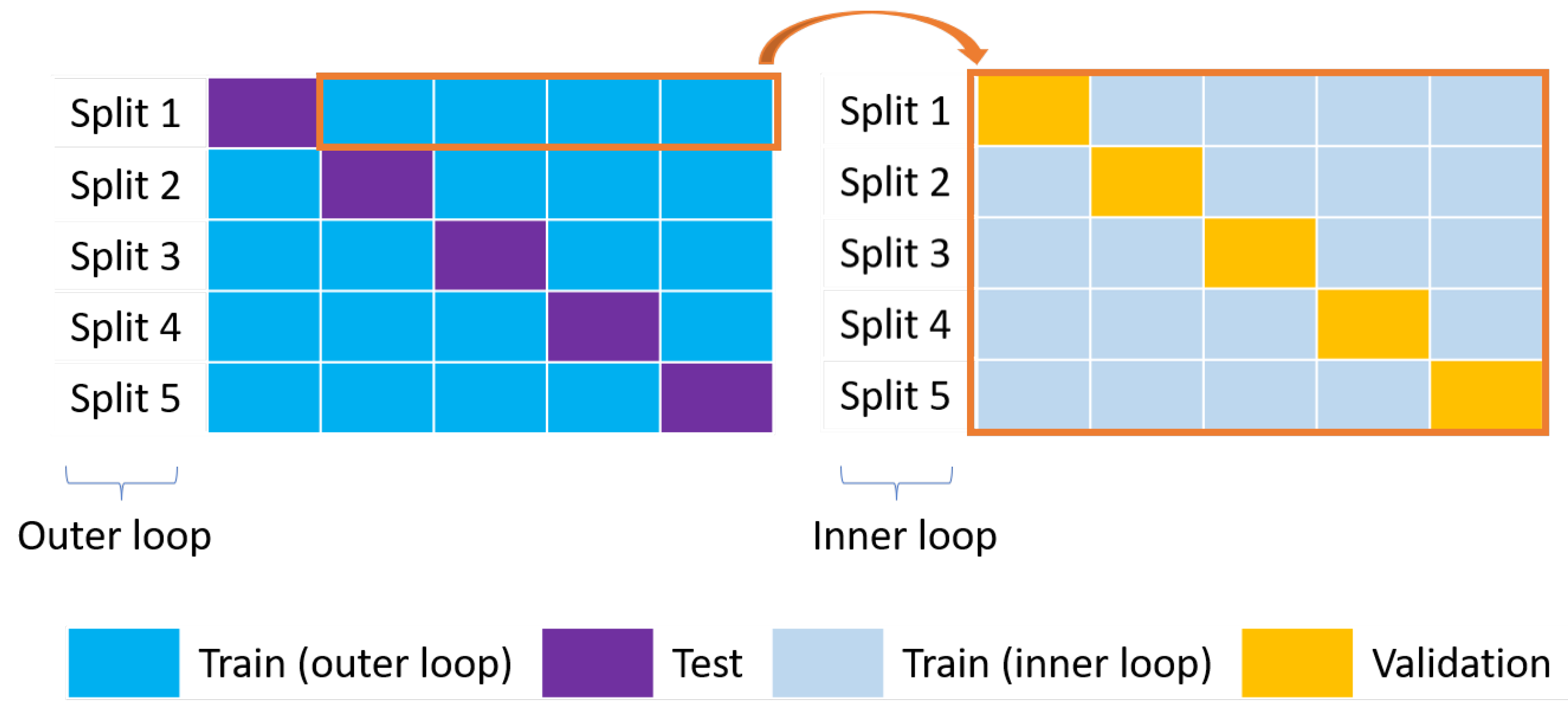
Processes 11 03325 g007
Figure 8. Nested CV. The outer loop on the left (blue and purple boxes for the training and test sets, respectively) is used for model selection while the inner loop on the right (grey and yellow boxes for the training and validation sets, respectively) is used for the optimization of the HPs.
Processes 11 03325 g008
Figure 9. Performance of the different ML models during the preliminary screening for the enthalpy: (a) R 2 ; (b) M A E ; (c) R M S E  (preprocessing: default, splitting: 5-fold external CV, scaling: standard, dimensionality reduction: none, HP optimization: none).
Processes 11 03325 g009
Figure 10. Parity plots of the selected ML models during the preliminary screening, for different splits, for the enthalpy (preprocessing: default, splitting: 5-fold external CV, scaling: standard, dimensionality reduction: none, HP optimization: none).
Processes 11 03325 g010aProcesses 11 03325 g010b
Figure 11. Distribution of the coefficients in various linear regression models during the preliminary screening, for split 1, for the enthalpy (preprocessing: default, splitting: 5-fold external CV, scaling: standard, dimensionality reduction: none, HP optimization: none).
Processes 11 03325 g011
Figure 12. Effect of the value of k’, for the external CV, on the (a) train M A E (b), test M A E , (c) training time, of the different ML models during the preliminary screening for the enthalpy (preprocessing: default, splitting: 5 and 10-fold external CV, scaling: standard, dimensionality reduction: none, HP optimization: none).
Processes 11 03325 g012
Figure 13. Effect of the data scaling technique on the (a) train M A E (b), test M A E , of the different ML models during the preliminary screening for the enthalpy (preprocessing: default, splitting: 5-fold external CV, scaling: standard/min-max/robust, dimensionality reduction: none, HP optimization: none). N.B. Robust scaler did not work with the SVR lin method (cf. red crosses).
Processes 11 03325 g013
Figure 14. Effect of the value of (a) the variance threshold (b) the correlation coefficient threshold, on the number of retained descriptors and Lasso model test M A E for the enthalpy (preprocessing: default for (a) and default with low variance threshold = 0.0001 for (b), splitting: 5-fold external CV, scaling: standard, dimensionality reduction: none, HP optimization: none).
Processes 11 03325 g014
Figure 15. Explained variance as a function of the principal components obtained with PCA for (a) the enthalpy and (b) the entropy. (preprocessing: final, splitting: 5-fold external CV, scaling: standard, dimensionality reduction: PCA, HP optimization: none).
Processes 11 03325 g015
Figure 16. Parity plots of the selected ML models after HP optimization, for different splits, for the enthalpy (preprocessing: final, splitting: 5-fold external CV, scaling: standard, dimensionality reduction: wrapper-GA Lasso, HP optimization: yes).
Processes 11 03325 g016aProcesses 11 03325 g016b
Figure 17. Parity plots of the selected ML models after HP optimization, for different splits, for the entropy (preprocessing: final, splitting: 5-fold external CV, scaling: standard, dimensionality reduction: wrapper-GA Lasso, HP optimization: yes).
Processes 11 03325 g017
Table 1. Classification of DIPPR data per uncertainty.
PropertyUncertainty
<0.2% <1% <3% <5% <10% <25% <50% <100% NaN
Enthalpy50401101324219718833419
Entropy66184101941918419920028
Table 2. AlvaDesc descriptors per category.
CategoryCategoryNumber ofCategoryCategoryNumber of
Name Descriptors Name Descriptors
1Constitutional indices5018WHIM descriptors114
2Ring descriptors3519GETAWAY descriptors273
3Topological indices7920Randic molecular profiles41
4Walk and path counts4621Functional group counts154
5Connectivity indices3722Atom-centred fragments115
6Information indices5123Atom-type E-state indices346
72D matrix-based descriptors60824Pharmacophore descriptors165
82D autocorrelations213252D Atom Pairs1596
9Burden eigenvalues96263D Atom Pairs36
10P_VSA-like descriptors6927Charge descriptors15
11ETA indices4028Molecular properties27
12Edge adjacency indices32429Drug-like indices30
13Geometrical descriptors3830CATS 3D descriptors300
143D matrix-based descriptors13231WHALES descriptors33
153D autocorrelations8032MDE descriptors19
16RDF descriptors21033Chirality descriptors70
173D-MoRSE descriptors224
Table 3. Summary of the tested and default preprocessing options.
Preprocessing StepTestedDefault
Elimination of Desc-MVs- By row
- By columnAlternating row or column
- Alternating row or column
Elimination of descriptors[0, 0.0001, 0.001, 0.01,0.001
with low variance0.1, 1, 10, 100, 1000]
Elimination of correlated[0.6, 0.7, 0.8, 0.9,0.95
descriptors0.92, 0.95, 0.98, 0.99]
Table 4. Methods tested for dimensionality reduction.
Feature ExtractionFeature Selection
Filter Wrapper Embedded
Pearson coefficientGALasso
PCAMISFSSVR lin
ET
Table 5. Configurations tested during ML model construction.
Data ScalingData SplittingML ModelsPerformance Metrics
Standard5-fold internal CVLRCoefficient of determination
x s c a l e d = x x ¯ σ x 5 and 10-fold external CVRidge R 2 = 1 ( y D I P P R y p r e d i c t e d ) 2 ( y D I P P R y D I P P R ¯ ) 2
Lasso
Min-Max SVR linRoot Mean Squared Error
x s c a l e d = x x m i n x m a x x m i n GP R M S E = 1 n ( y D I P P R y p r e d i c t e d ) 2
kNN
Robust DTMean Absolute Error
x s c a l e d = x Q 2 Q 3 Q 1 RF M A E = 1 n y D I P P R y p r e d i c t e d
ET
AB
GB
MLP
Table 6. Configurations selected for the study of the effects of data preprocessing and dimensionality reduction, and for HP optimization.
Data ScalingData SplittingML ModelsPerformance Metrics
Standard5-fold external CVLasso M A E
SVR lin
ET
MLP
Table 7. Effect of the algorithms for the elimination of Desc-MVs on the data set size and Lasso model test M A E for the enthalpy (preprocessing: default, splitting: 5-fold external CV, scaling: standard, dimensionality reduction: none, HP optimization: none).
EliminationData SetData SetData Set afterMAE TrainMAE Test
Procedure with Desc-MVs without Desc-MVs Preprocessing (kJ/mol) (kJ/mol)
Alg.1: by row1903 × 5666236 × 5666236 × 13787.6 ± 0.4 20.4 ± 6.4
mol.   desc.0 duplicates
Alg.2: by column1903 × 56661903 × 28551903 × 98821.1 ± 1.0 32.9 ± 5.9
73 duplicates
Alg.3: alternating1903 × 56661785 × 55311785 × 196116.7 ± 0.4 27.6 ± 1.7
row or column0 duplicates
mol.: molecules. desc.: descriptors. Blue, orange and red colors represent limited, moderate, important information loss, respectively. In column 3, the amount of duplicated rows is indicated in italics. In columns 5 and 6, the standard deviation over the different splits is provided in subscript.
Table 8. Summary of the final preprocessing options.
Preprocessing StepFinal
Elimination of Desc-MVsAlternating row or column
Elimination of descriptors with low variance0.0001
Elimination of correlated descriptors 0.98
Table 9. Effect of the different dimensionality reduction methods on the test M A E of the selected ML models for the enthalpy (preprocessing: final, splitting: 5-fold external CV, scaling: standard, dimensionality reduction: different methods, HP optimization: none).
Dimensionality Reduction MethodNb of Desc.Time/Split (s)MAE Test (kJ/mol)Nb ofNb of Desc.
Lasso SVR lin ET MLP Pairwise Correlations ≥ 0.9 with Variance ≤ 0.01
None (reference case)2506027.0 ± 1.7 28.6 ± 3.6 42.6 ± 6.6 37.9 ± 5.2 4473512
Filter-Pearson10019.461.6  ± 2.5 75.0  ± 5.7 56.7  ± 6.1 116.0  ± 3.6 1242
Filter-MI10018.755.8  ± 3.6 62.5  ± 7.8 43.8  ± 7.8 90.8  ± 9.8 724
Wrapper-SFS Lasso100779531.1  ± 2.4 34.9  ± 3.3 42.9  ± 4.8 84.6  ± 3.7 321
Wrapper-GA Lasso1004957324.2  ± 4.0 31.0  ± 5.0 43.8  ± 5.2 76.1  ± 9.7 526
Embedded-Lasso1001.529.0  ± 1.4 29.0  ± 2.4 38.8  ± 5.5 88.7  ± 9.9 1424
Embedded-SVR lin1007.039.8  ± 5.1 40.0  ± 5.6 41.1  ± 6.1 84.1  ± 4.2 3418
Embedded-ET1003.750.3  ± 4.1 51.2  ± 4.0 41.4  ± 5.9 85.5  ± 9.0 464
PCA 95% (261–265 PC)25062.937.3  ± 3.3 34.2  ± 2.7 76.8  ± 12.1 38.0  ± 2.2 --
Table 10. Top five descriptor categories identified by the different dimensionality reduction methods for the enthalpy (preprocessing: final, splitting: 5-fold external CV, scaling: standard, dimensionality reduction: different methods, HP optimization: none). The percentages correspond to the proportion of a descriptor category among the descriptors obtained with each method.
Dimensionality Reduction MethodTop 5 Descriptor Categories
None (reference case)25 13.0 % 19 8.5 % 8 7.2 % 30 6.3 % 17 6.3 %
Filter-Pearson8 24.4 % 3 16.6 % 16 15.4 % 19 13.2 % 7 8.2 %
Filter-MI8 21.4 % 7 19.2 % 3 13.0 % 11 9.8 % 27 8.6 %
Wrapper-SFS Lasso25 16.8 % 23 10.6 % 22 9.0 % 21 6.6 % 17 6.0 %
Wrapper-GA Lasso25 22.6 % 23 10.4 % 22 9.2 % 21 8.4 % 10 8.2 %
Embedded-Lasso25 20.8 % 22 8.4 % 7 7.6 % 10 7.4 % 23 7.4 %
Embedded-SVR lin25 32.2 % 23 9.8 % 10 8.8 % 22 7.8 % 1 7.2 %
Embedded-ET12 16.0 % 8 13.6 % 7 13.4 % 3 8.6 % 11 7.2 %
PCA 95% (261–265 PC)25 13.0 % 19 8.5 % 8 7.2 % 30 6.3 % 17 6.3 %
Table 11. Effect of the different dimensionality reduction methods on the test M A E of the selected ML models for the entropy (preprocessing: final, splitting: 5-fold external CV, scaling: standard, dimensionality reduction: different methods, HP optimization: none).
Dimensionality Reduction MethodNb of Desc.Time/Split (s)MAE Test (J/mol/K)Nb ofNb of Desc.
Lasso SVR lin ET MLP Pairwise Correlations ≥ 0.9 with Variance ≤ 0.01
None (reference case)2479018.7 ± 1.1 24.3 ± 2.2 19.6 ± 1.4 27.1 ± 1.6 4469487
Filter-Pearson10018.120.9  ± 1.3 18.5  ± 1.7 20.3  ± 1.3 46.9  ± 3.0 9092
Filter-MI10016.321.4  ± 1.4 19.1  ± 1.4 20.0  ± 1.6 31.4  ± 1.0 5146
Wrapper-SFS Lasso100829419.2  ± 1.2 18.9  ± 1.7 19.6  ± 1.9 55.8  ± 4.2 1519
Wrapper-GA Lasso10053,31517.4  ± 1.2 18.1  ± 1.3 19.6  ± 1.5 57.5  ± 3.7 925
Embedded-Lasso1001.418.8  ± 1.1 18.5  ± 1.2 19.7  ± 1.5 52.6  ± 5.6 2120
Embedded-SVR lin1005.624.2  ± 2.5 23.5  ± 2.8 21.3  ± 2.0 53.0  ± 4.6 817
Embedded-ET1003.721.6  ± 1.9 19.7  ± 1.4 20.8  ± 2.1 31.0  ± 1.7 3388
PCA 95% (254–260 PCs)24793.019.7  ± 1.0 18.3  ± 1.5 23.0  ± 1.3 29.1  ± 2.3 --
Table 12. Top 5 descriptor categories identified by the different dimensionality reduction methods for the entropy (preprocessing: final, splitting: 5-fold external CV, scaling: standard, dimensionality reduction: different methods, HP optimization: none).
Dimensionality Reduction MethodTop 5 Descriptor Categories
None (reference case)25 12.9 % 19 8.7 % 8 7.2 % 17 6.3 % 30 6.2 %
Filter-Pearson7 16.2 % 16 15.8 % 19 15.4 % 3 7.0 % 14 7.0 %
Filter-MI7 46.8 % 14 10.6 % 3 8.4 % 8 6.2 % 1 4.0 %
Wrapper-SFS Lasso25 14.6 % 30 10.4 % 21 7.0 % 7 6.0 % 24 5.4 %
Wrapper-GA Lasso25 16.6 % 21 10.4 % 30 7.0 % 24 5.4 % 7 5.0 %
Embedded-Lasso25 17.2 % 21 9.6 % 16 8.0 % 30 7.8 % 23 6.0 %
Embedded-SVR lin25 15.8 % 30 12.0 % 16 8.0 % 24 7.4 % 21 6.4 %
Embedded-ET7 28.2 % 8 14.6 % 14 11.8 % 9 9.8 % 19 8.4 %
PCA 95% (254–260 PCs)25 12.9 % 19 8.7 % 8 7.2 % 17 6.3 % 30 6.2 %
Table 13. HP optimization settings and results for the selected ML models for the enthalpy (preprocessing: final, splitting: 5-fold external CV, scaling: standard, dimensionality reduction: wrapper-GA Lasso, HP optimization: yes).
MLHPsScreening RangesOptimal HP Settings per Split
Model (Blue = Default Value) Split 1 Split 2 Split 3 Split 4 Split 5
Lassoalpha[0.001, 0.01, 0.1, 0.5, 1, 1.5, 2]0.10.0010.10.50.1
kernel[‘linear’]linearlinearlinearlinearlinear
SVR linC[0.1, 0.5, 1, 1.5, 2]22222
epsilon[0.01, 0.1, 1]0.10.1111
n_estimators[50, 100, 200]200200100100200
max_features[‘sqrt’, ‘log2’, None]NoneNoneNoneNoneNone
min_samples_split[2, 5]22222
ETmin_samples_leaf[1, 5]11111
max_depth[10, None]NoneNoneNoneNoneNone
criterion[‘absolute error’,squaredsquaredsquaredsquaredsquared
‘squared error’]
activation[‘relu’]relurelurelurelurelu
hidden_layer_sizes1 hidden layer: [(i)],(100)(10,10)(15,15)(10,10)(15,15)
i = 100, 200, 400;
MLP 2 hidden layers: [(i, i)],
i = 10, 15, 20
solver[‘adam’, ‘lbfgs’]lbfgslbfgslbfgslbfgslbfgs
learning_rate_init[0.001, 0.01, 0.1, 0.5]0.0010.0010.0010.0010.001
max_iter[200, 500]200500500200200
Table 14. Performance of the selected ML models with and without HP optimization for the enthalpy (preprocessing: final, splitting: 5-fold external CV, scaling: standard, dimensionality reduction: wrapper-GA Lasso, HP optimization: none/yes).
ModelData Set R 2 MAE (kJ/mol)RMSE (kJ/mol)
HP Not Opt. HP Opt. HP Not Opt. HP Opt. HP Not Opt. HP Opt.
LassoTrain (internal)0.995 ± 0.001 0.996 ± 0.001 15.8 ± 0.5 14.6 ± 0.3 35.9 ± 1.4 33.7 ± 1.5
Validation0.987 ± 0.002 0.989 ± 0.002 24.8 ± 1.5 22.3 ± 0.7 52.2 ± 3.5 47.8 ± 2.9
Train (external)0.995 ± 0.001 0.996 ± 0.001 15.5 ± 0.5 14.6 ± 0.3 36.9 ± 1.5 34.6 ± 1.6
Test0.978 ± 0.016 0.976 ± 0.019 24.2 ± 4.0 25.1 ± 4.1 70.8 ± 23.1 74.2 ± 25.9
SVR linTrain (internal)0.987 ± 0.005 0.993 ± 0.002 23.1 ± 3.3 17.9 ± 1.6 58.2 ± 11.9 44.6 ± 6.0
Validation0.975 ± 0.008 0.984 ± 0.006 35.6 ± 5.3 27.8 ± 2.9 75.6 ± 15.9 60.1 ± 9.9
Train (external)0.990 ± 0.004 0.993 ± 0.002 21.4 ± 2.5 17.3 ± 1.6 53.5 ± 9.6 43.7 ± 5.8
Test0.968 ± 0.023 0.971 ± 0.021 31.0 ± 5.0 27.8 ± 4.5 85.8 ± 26.8 82.4 ± 26.3
ETTrain (internal)1.000 ± 0.000 1.000 ± 0.000 0.0 ± 0.0 0.0 ± 0.0 0.0 ± 0.0 0.0 ± 0.0
Validation0.933 ± 0.006 0.933 ± 0.006 61.6 ± 4.9 61.3 ± 4.6 114.5 ± 9.3 114.4 ± 9.2
Train (external)1.000 ± 0.000 1.000 ± 0.000 0.0 ± 0.0 0.0 ± 0.0 0.0 ± 0.0 0.0 ± 0.0
Test0.955 ± 0.014 0.955 ± 0.014 43.8 ± 5.2 43.6 ± 5.5 112.3 ± 36.1 112.3 ± 36.7
MLPTrain (internal)0.955 ± 0.006 0.998 ± 0.001 79.7 ± 7.2 11.8 ± 3.7 112.2 ± 10.5 20.1 ± 6.5
Validation0.764 ± 0.016 0.964 ± 0.009 125.9 ± 6.7 42.5 ± 2.7 197.0 ± 11.9 81.3 ± 6.6
Train (external)0.968 ± 0.005 0.999 ± 0.000 65.2 ± 8.1 10.3 ± 2.4 95.3 ± 10.9 17.7 ± 3.8
Test0.943 ± 0.025 0.976 ± 0.008 76.1 ± 9.7 34.9 ± 2.5 117.6 ± 12.9 78.3 ± 10.9
Table 15. Performance of Lasso model with HP optimization for the entropy (preprocessing: final, splitting: 5-fold external CV, scaling: standard, dimensionality reduction: wrapper-GA Lasso, HP optimization: yes).
ModelData Set R 2 MAE (J/mol/K)RMSE (J/mol/K)
LassoTrain (internal)0.982 ± 0.001 13.8 ± 0.4 27.6 ± 0.9
Validation0.966 ± 0.005 17.5 ± 0.6 34.5 ± 1.8
Train (external)0.982 ± 0.001 13.7 ± 0.4 28.0 ± 0.9
Test0.968 ± 0.008 17.9 ± 1.2 36.2 ± 4.3
Table 16. a Hydrocarbons, oxygenated, nitrogenated, chlorinated, fluorinated, brominated, iodinated, phosphorus containing, sulfonated, silicon containing, multifunctional. b GroupGAT (group-contribution-based graph attention). c Probabilistic vector learned from interatomic distances, bond angles, and dihedral angles histograms with GMM (Gaussian Mixture Model). N/A: not available.
PropertyReferenceData SourceType of MoleculesNb of MoleculesMolecular RepresentationML Model R 2 Test MAE TestRMSE Test k
H (kJ/mol)[109]DIPPR exp.Diverse a 741GNN b GNN b 0.9918.630.510
This work100 descriptorsLasso0.9912.421.6
[51]Literature exp., ab initioNoncyclic hydrocarbons310261 descriptorsSVR0.9955.703N/A10
This work100 descriptorsLasso0.9984.4266.520
[52]Literature exp.Cyclic hydrocarbons19247 descriptorsSVR0.9869.71N/A10
[56]GauL HDAD c ANNN/A9.612.9
This work100 descriptorsLasso0.98510.0114.51
[56]Lignin QM ab initio(Poly)cyclic hydrocarbons and oxygenates3926GauL HDAD c ANNN/A9.3415.8910
This work100 descriptorsLasso0.9821.4830.81
[110]SPEED exp.Diverse1059240 groupsGP0.987N/A42.7420
This work100 descriptorsLasso0.97611.3028.20
S (J/mol/K)[56]Lignin QM ab initio(Poly)cyclic hydrocarbons and oxygenates3926GauL HDAD c ANNN/A3.865.3210
This work100 descriptorsLasso0.995.577.43
[53]Literature exp., theo.Hydrocarbons310252 descriptorsSVR0.996.3910
This work100 descriptorsLasso0.988.310.8
[111]DIPPR exp.Organic511GNNGNN0.995.3N/A10
This work100 descriptorsLasso0.996.19.4
Disclaimer/Publisher’s Note: The statements, opinions and data contained in all publications are solely those of the individual author(s) and contributor(s) and not of MDPI and/or the editor(s). MDPI and/or the editor(s) disclaim responsibility for any injury to people or property resulting from any ideas, methods, instructions or products referred to in the content.

