Vibration Response of the Interfaces in Multi-Layer Combined Coal and Rock Mass under Impact Load

Abstract

The stress wave generated by impact or dynamic load will produce significant reflection and transmission at the rock coal or rock interface during the propagation process. This will produce dynamic effects such as dynamic tensile, stress superposition and mutation. These dynamic effects will lead to obvious vibration at the interfaces, which is a key factor leading to dynamic damage and the failure of coal and rock mass. In the process of underground engineering excavation, the dynamic damage of a series of layered rock masses is one of the important factors causing geological disasters. Based on the two–dimensional similar material simulation experiment, the coal and rock mass combined of five layers of fine sandstone, medium sandstone, coal, coarse sandstone and mudstone was taken as the research object, and single and multi-point excitation (synchronous/step-by-step) were used to test the time–history vibration curves of rock–coal and rock–rock interfaces under impact load. It was concluded that the change of extreme value of vibration amplitude presented two stages: first increase, and then attenuation. Most of them required 2.25 cycles to reach the peak value, and the dynamic attenuation of amplitude conformed to the law of exponential. Based on Fast Fourier transform (FFT), the spectrum structures of the amplitude–frequency of interface vibration were studied, and the two predominant frequencies were 48.9~53.7 Hz and 92.4 Hz, respectively. Based on the Hilbert-Huang transform and energy equation, 5~7 vibration modes (IMF) were obtained by decomposing the time–history curves. The three modes, IMF1, IMF2, and IMF3, contained high energy and were effective vibration modes. IMF2 accounted for the highest proportion and was the main vibration mode whose predominant frequencies were concentrated in 45.6~50.2 Hz. Therefore, IMF2 played a decisive role in the whole vibration process and had an important impact on the dynamic response, damage and failure of coal and rock mass. In real conditions, the actual predominant frequencies can be converted according to the size and mechanical properties of the coal and rock mass, and the vibration response characteristics of the interfaces between coal and rock mass under impact load were preliminarily revealed. This study can provide reference for monitoring and early warning of coal and rock dynamic disasters, prevention and control of coal and gas outburst and technical development.

1. Introduction

The sedimentary process and the arrangement of mineral particles during the formation of coal measure rock mass give an obvious bedding structure and show layered structure macroscopically [1,2,3]. This layered rock mass widely exists in mining, construction, transportation and water conservancy projects [4,5,6], and is prone to vibration, damage and even failure under the action of external dynamic disturbances, such as blasting, roof and floor breaking, rock instability and so on [7,8]. For example, the roof strata of working face in mines, especially in the early stage of mining, is subjected to the loading/unloading action of dynamic disturbance and the appearance of mineral pressure is violent, which leads to obvious mine earthquakes and even roof collapse. Therefore, in the process of underground engineering excavation, the dynamic damage of a series of layered rock masses is one of the most important factors causing geological disasters.

At present, scholars in China and other countries have mainly studied the static mechanical properties of single, two-layer or three-layer combined coal and rock mass. Zuo et al. demonstrated that both the breaking strength and elastic modulus of the coal–rock assemblage increased to some extent compared with the single coal sample, with the rock–coal–rock assemblage having the largest breaking strength and elastic modulus [9]. Li et al. demonstrated that more than one peak was observed in the spectrum of green sandstone with repeated impact loads, and the relative weight of peak frequencies increased in the low frequency range [10]. Mu et al. demonstrated that the damage state of coal rock specimens was determined by the post peak stiffness of the coal in relation to the rock stiffness [11]. Liu et al. demonstrated that the dynamic strength and fragmentation dimension of the combined coal rock specimens increased with increasing stress wave energy and showed a trend of first increasing and then decreasing with static load [12]. However, the research on dynamic response, the vibration characteristics and dynamic damage of coal and rock mass, especially multi-layer combined coal and rock mass, are still in the stage of experimental exploration. The stress wave generated by impact or dynamic load has significant reflection and transmission at the rock–coal or rock–rock interfaces in the process of propagation, resulting in dynamic effects such as dynamic tensile, stress superposition and mutation. These dynamic effects lead to obvious vibration at the interfaces, which is a key factor leading to dynamic damage and failure of coal and rock mass [13,14,15,16]. Meanwhile, Li et al. demonstrated that the initial location of damage and failure can be determined by the lowest frequency effective vibration mode [17]. These articles illustrate that the study of coal rock vibration signals can help to initially reveal the vibration response characteristics of the coal rock interface under impact loading. Unlike previous studies on the static response characteristics of combined coal and rock mass below three layers, this paper conducts a study on the dynamic response characteristics of five-layer combined coal and rock mass.

Based on the two-dimensional similar material simulation experiment, the coal and rock mass combined by five layers of fine sandstone, medium sandstone, coal, coarse sandstone and mudstone was taken as the research object, single and multi-point excitation (synchronous/step-by-step) were used to test the time–history vibration curves of rock–coal and rock–rock interfaces under impact load, and the dynamic attenuation law of amplitude was obtained. Based on Fast Fourier transform (FFT), the spectrum structures of amplitude–frequency of interfaces vibration were studied. Based on Hilbert-Huang transform and energy equation, the time–history curves were decomposed by Ensemble Empirical Mode Decomposition (EEMD) and the vibration modes were obtained. According to the distribution laws of marginal spectrum and energy proportion, the most effective and main vibration modes and the predominant frequencies were obtained. The vibration response characteristics of the interfaces between coal and rock mass under impact load were preliminarily revealed.

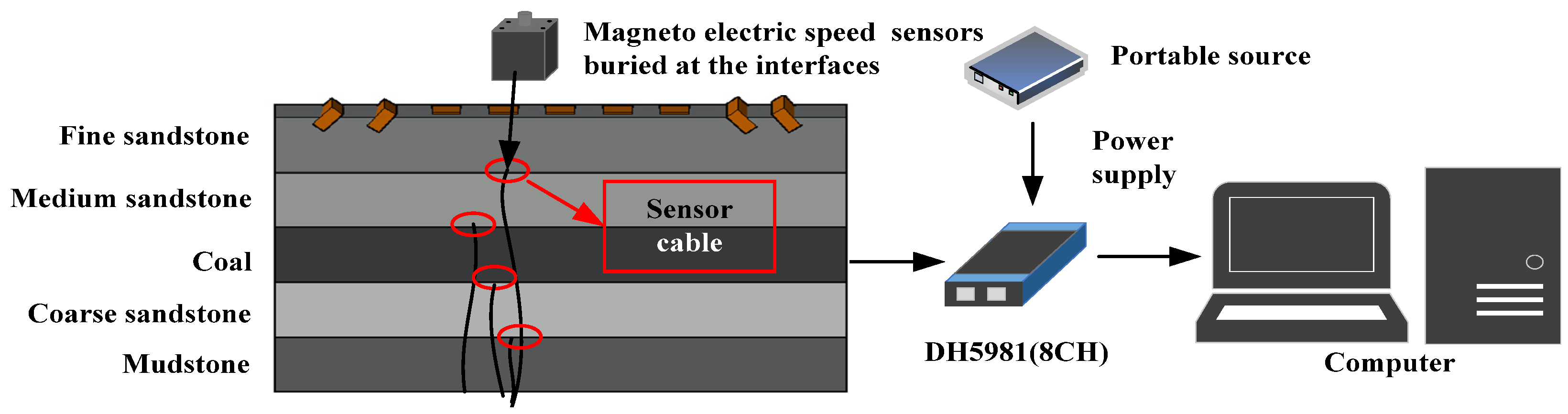
2. Experimental Design

2.1. Experimental Model

The two-dimensional similar material simulation experiment platform was often used to simulate the deformation, damage and failure laws of overlying strata in the process of mining [18,19]. The size of similar material simulation experiment platform was 1800 × 160 × 1100 mm in the lab. The multi-layer combined coal and rock mass was composed of five layers, each with a thickness of 200 mm; from top to bottom, they were fine sandstone, medium sandstone, coal, coarse sandstone and mudstone. The similarity density constant of rock mass is 1.6, and that of coal is 1; the composition and ratio of similar materials of each layer in coal and rock mass can be seen in

Table 1. The composition and ratio of similar materials of each layer.

Serial Number	Layers of Coal and Rock Mass	Raw Material Compressive Strength (MPa)	Similar Material Compressive Strength (MPa)	Fine Sand (Kg)	Cement (Kg)	Gypsum (Kg)	Water (Kg)
1	Fine sandstone	120	0.75	72.98	7.30	17.03	9.73
2	Medium sandstone	80.1	0.50	81.09	8.11	8.11	9.73
3	Coal	10	0.063	86.49	7.57	3.24	9.73
4	Coarse sandstone	61.5	0.384	83.40	6.95	6.95	9.73
5	Mudstone	27.4	0.171	88.46	6.32	6.32	10.11

. The vibration amplitude was measured by magnetoelectric speed sensors (2D001) with a size of 63 × 63 × 63 mm. The distributed network dynamic signal test system (DH5981) was used for data acquisition and analysis, as shown in Figure 1.

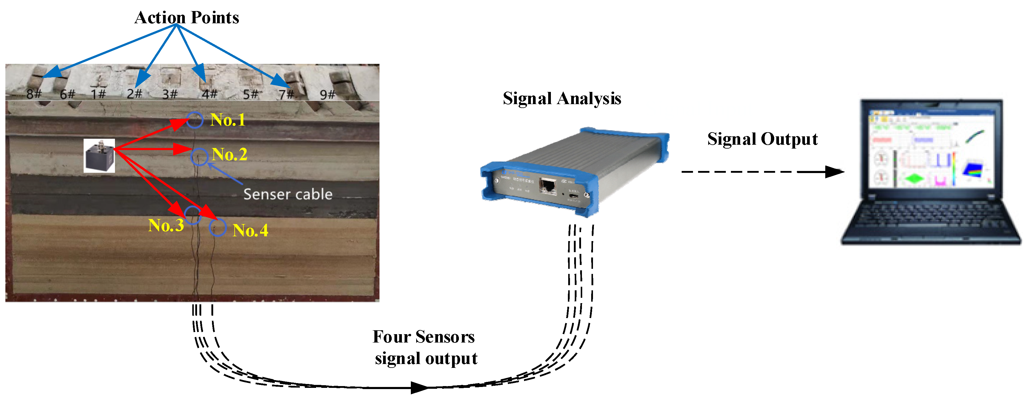
2.2. Action Points and Sensors Distribution

Four sensors (No. 1–4) were distributed at the interfaces of each layer of combined coal and rock mass, and each sensor was at the midpoint of each interface. The lower surface of the sensor (signal receiving surface) coincided with each interface of coal and rock mass. An action point was set every 100 mm on the upper surface of the fine sandstone for percussion excitation. An iron block of 80 × 80 mm was placed at action points to prevent damage to fine sandstone during excitation; a total of five vertical action points (1–5#) and four inclined action points with an angle of 45° to the horizontal direction (6–9#) were arranged, as shown in Figure 2.

2.3. Experimental Process

Single point and multi-point excitation (synchronous/step-by-step) were used in the experiment, and the specific excitation steps were as follows:

(1) the action point (1~9#) was excited respectively; (2) two action points were executed synchronously or step-by-step as follows: 1# and 2#, 1# and 5#, 2# and 4# (excitation step-by-step), 6# and 7#, 6# and 8#, 7# and 8#, 8# and 9#; (3) four action points (6~9#) and five action points (1~5#) were excited synchronously and respectively.

Before the experiment, the data acquisition instrument needed to be zeroed first, and when the impact actions caused by the excitation were balanced, the data acquisition would be terminated and saved.

3. Experimental Results

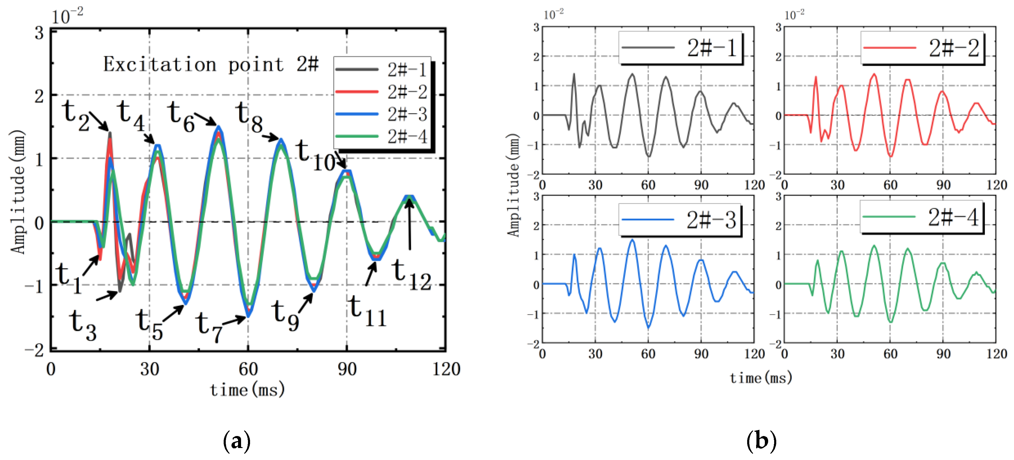
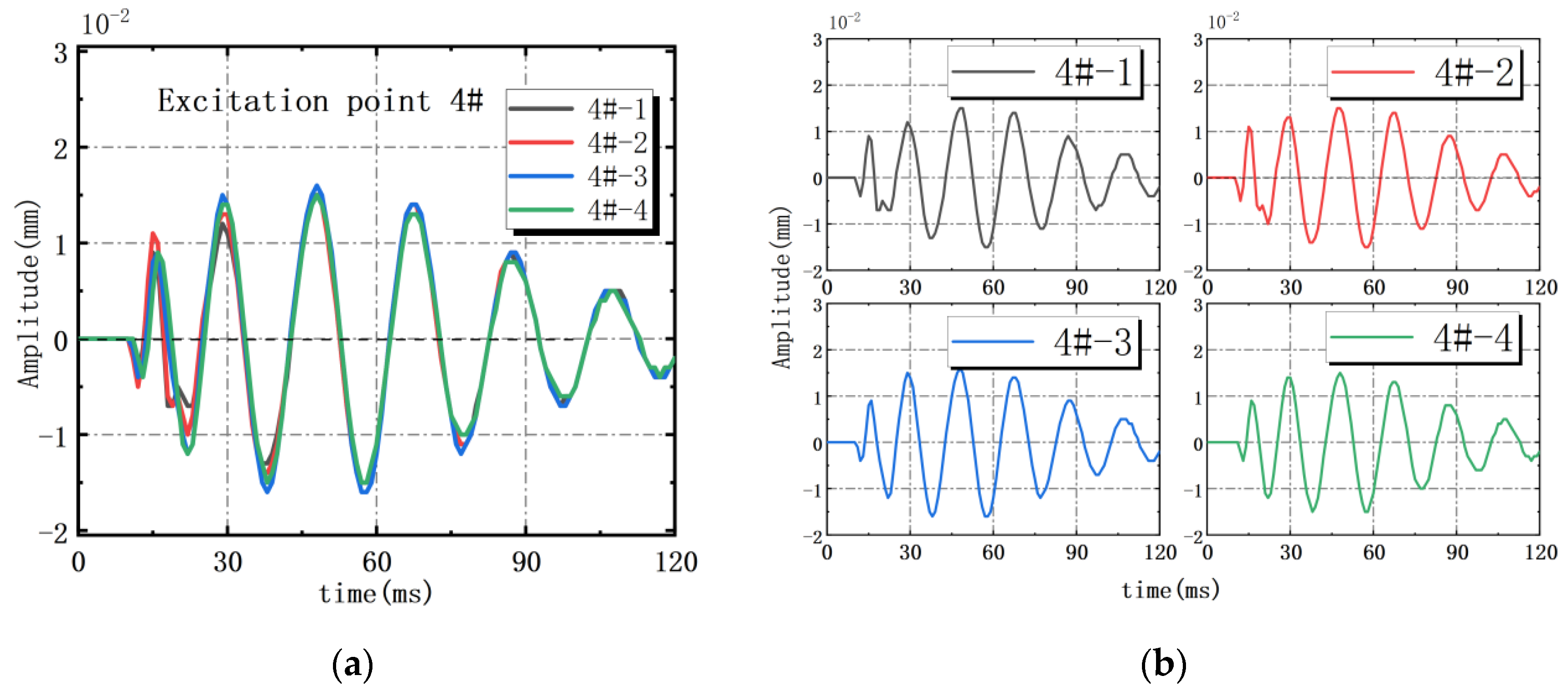
3.1. Amplitude Variation of Interface Vibration under Impact Load

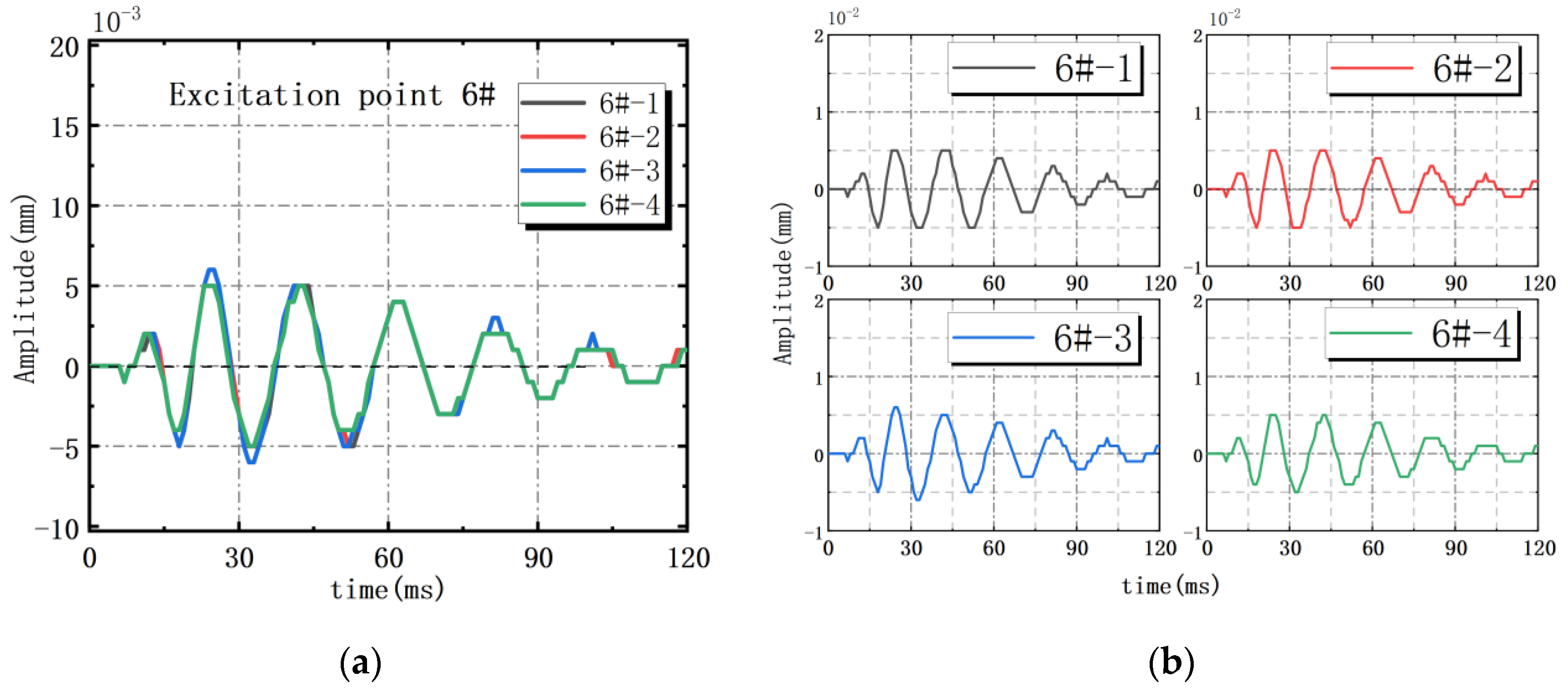
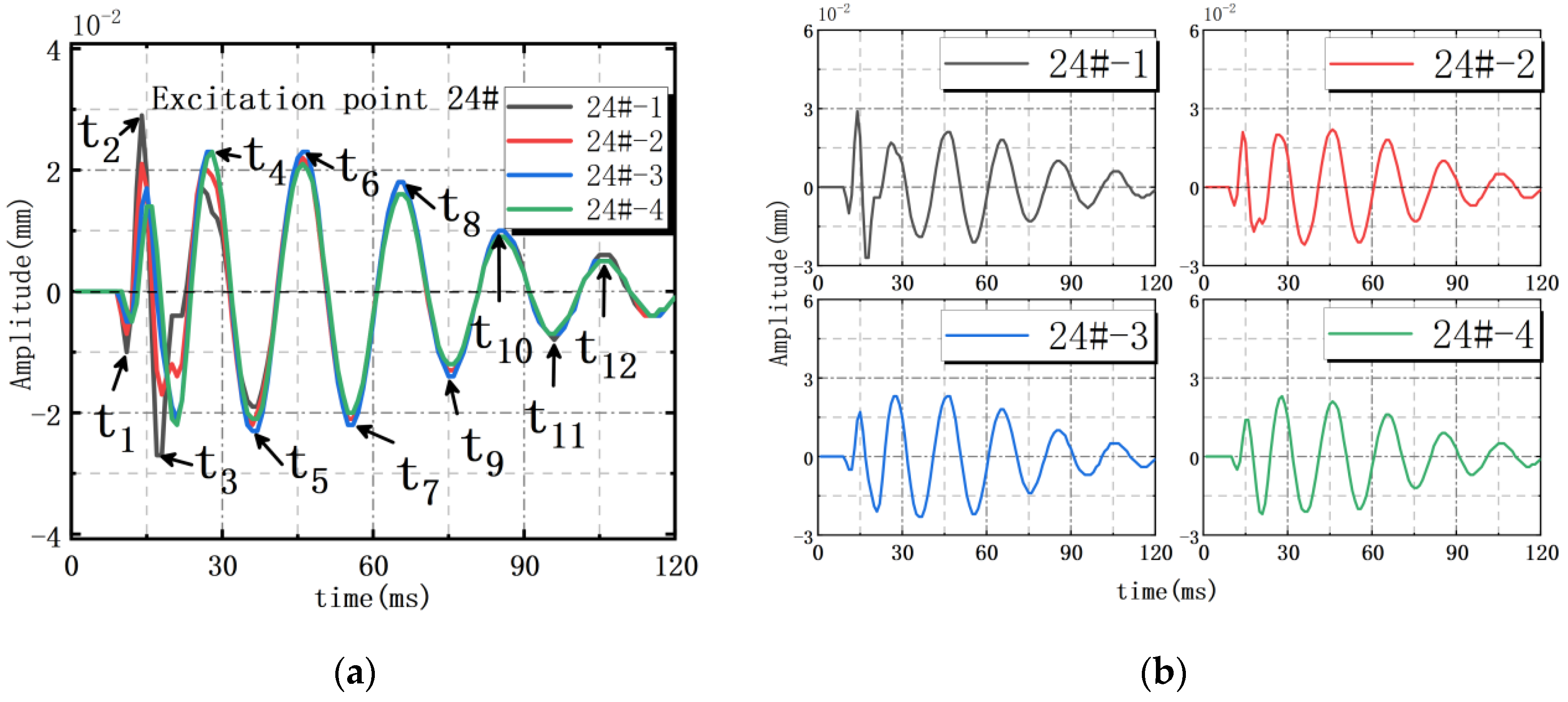
3.1.1. Amplitude Variation of Interface Vibration under Single Point Excitation

When a single point was excited, the dynamic variation laws of the vibration amplitude of each interface obtained from the four sensors were similar; the amplitude time-history curves of 2#, 4# and 6# action points excited separately are shown in Figure 3, Figure 4 and Figure 5. It can be seen from Figure 3 that when the 2# action point was excited alone, the amplitude curve (2#-1 in Figure 3) of No. 1 reached the first extreme value s₁ = −0.005 mm when t₁ = 15 ms and reached a peak s₆ = 0.014 mm when t₆ = 51 ms. When 4# action point was excited alone (Figure 4), the amplitude curve of No. 1 (2#-1 in Figure 4) reached the first extreme value s₁ = −0.004 mm when t₁ = 12 ms and the peak s₆ = 0.015 mm when t₆ = 49 ms. Similarly, when 6# action point was excited alone (Figure 5), the amplitude curve of No. 1 (6#-1 in Figure 5) reached the first extreme value s₁ = −0.001 mm when t₁ = 7 ms and the peak value s₆ = 0.005 mm when t₆ = 18 ms. The extreme points of amplitude curves of single point excitation (2#, 4# and 6#) and their corresponding time can be seen in

Table 2. The extreme points of amplitude curves of 2#, 4# and 6# action points.

Extreme Value (mm)/Time (ms)	2#	4#	6#
s1/t1	0.005/15	0.004/12	0.001/7
s2/t2	0.014/18	0.009/15	0.002/13
s3/t3	0.011/21	0.007/22	0.005/18
s4/t4	0.010/33	0.012/29	0.005/25
s5/t5	0.011/42	0.013/38	0.005/33
s6/t6	0.014/51	0.015/49	0.005/43
s7/t7	0.014/61	0.015/58	0.005/52
s8/t8	0.013/70	0.014/67	0.004/62
s9/t9	0.011/80	0.011/78	0.003/72
s10/t10	0.008/90	0.008/86	0.003/82
s11/t11	0.006/99	0.007/97	0.002/92
s12/t12	0.004/109	0.004/117	0.002/101

. The extreme values of the amplitude curves of these three action points showed two stages as follows: first increasing and then decreasing; the vibration curves of 2# and 4# action points reached the peak after 2.25 cycles, and that of 6# action point the peak after 1.25 cycles.

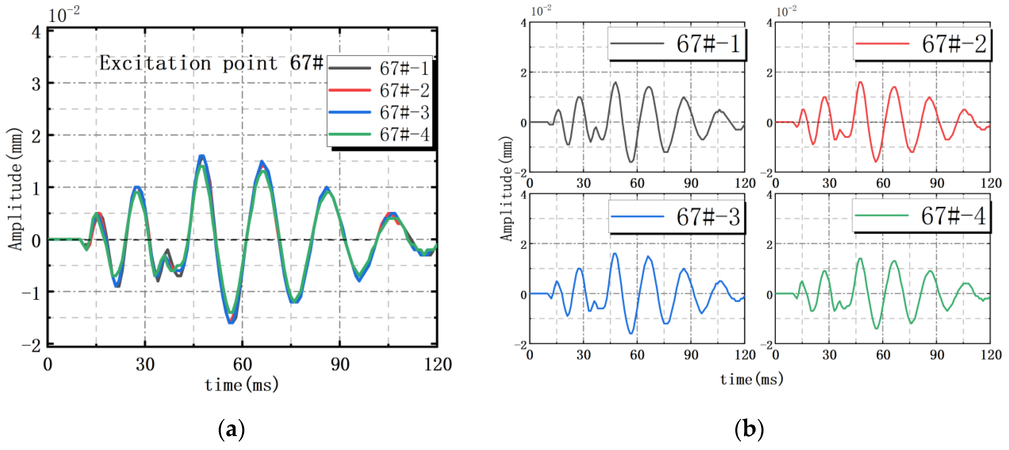
3.1.2. Amplitude Variation of Interface Vibration under Multi-Point Excitation

When 2# and 4# action points were excited step-by-step, the curve of No. 1 (24#-1 in Figure 6) reached the first extreme value s₁ = −0.01 mm when t₁ = 11 ms, the peak s₂ = 0.029 mm when t₂ = 14 ms, and the second peak s₆ = 0.021 mm when t₆ = 46 ms. Compared with No. 3 and No. 4, No. 1 and No. 2 were close to the action points, and there were complex micro vibrations during step-by-step excitation (24#-1 and 24#-2 in Figure 6), but the whole dynamic change of all measuring points were similar. When 6# and 7# action points were excited synchronously, the curve of No. 1 (67#-1 in Figure 7) reached the first extreme value s₁ = −0.001 mm when t₁ = 12 ms, the peak s₆ = 0.016 mm when t₆ = 48 ms, and the whole dynamic change of all measuring points were also similar. The extreme values of the amplitude curves of these two groups of action points showed two stages as follows: first increasing and then decreasing, and the vibration curves reached the peak after 2.25 cycles. The extreme points of amplitude curves of multi-point excitation (2# and 4#, 6# and 7#) and their corresponding time could be seen in

Table 3. The extreme points of amplitude curves of two groups of action points (2# and 4#, 6# and 7#).

Extreme Value (mm)/Time (ms)	2# and 4#	6# and 7#
s1/t1	0.010/11	0.001/12
s2/t2	0.029/14	0.004/17
s3/t3	0.027/18	0.009/22
s4/t4	0.016/27	0.010/28
s5/t5	0.019/37	0.008/34
s6/t6	0.021/47	0.016/48
s7/t7	0.021/56	0.016/57
s8/t8	0.018/66	0.014/67
s9/t9	0.013/76	0.012/77
s10/t10	0.010/86	0.010/86
s11/t11	0.008/96	0.007/97
s12/t12	0.006/107	0.005/106

.

3.2. Amplitude Attenuation Law of Interface Vibration under Impact Load

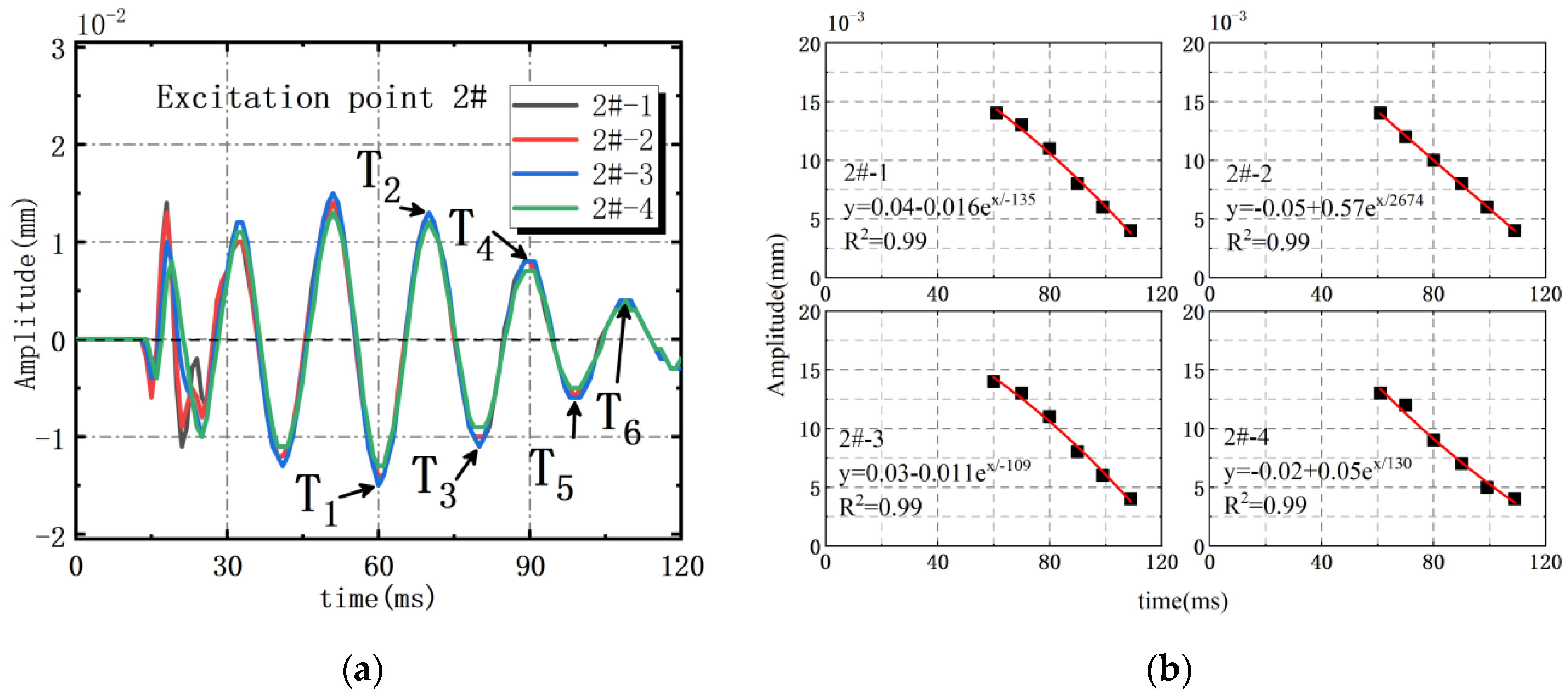
3.2.1. Dynamic Attenuation Law of Amplitude under Single Point Excitation

The analysis results of the amplitude extreme value under single point excitation showed that the dynamic changes were similar. The extreme values distribution of the test curves when 6# action point was excited alone can be seen in

Table 4. Amplitude extreme points of No. 1–4 under 2# action point excitation.

Extreme Point	Time (ms)	No. 1 (mm)	Time (ms)	No. 2 (mm)	Time (ms)	No. 3 (mm)	Time (ms)
T1	61	0.014	61	0.014	60	0.014	61
T2	70	0.013	70	0.012	70	0.013	70
T3	80	0.011	80	0.01	80	0.011	80
T4	90	0.008	90	0.008	90	0.008	90
T5	99	0.006	99	0.006	99	0.006	99

, and the curve–fitting results are shown in Figure 8. It could be concluded that the dynamic attenuation of amplitude under single point excitation conformed to the law of exponential variation y = y0 + Aexp (x/k), and the fitting degree was as high as 0.99.

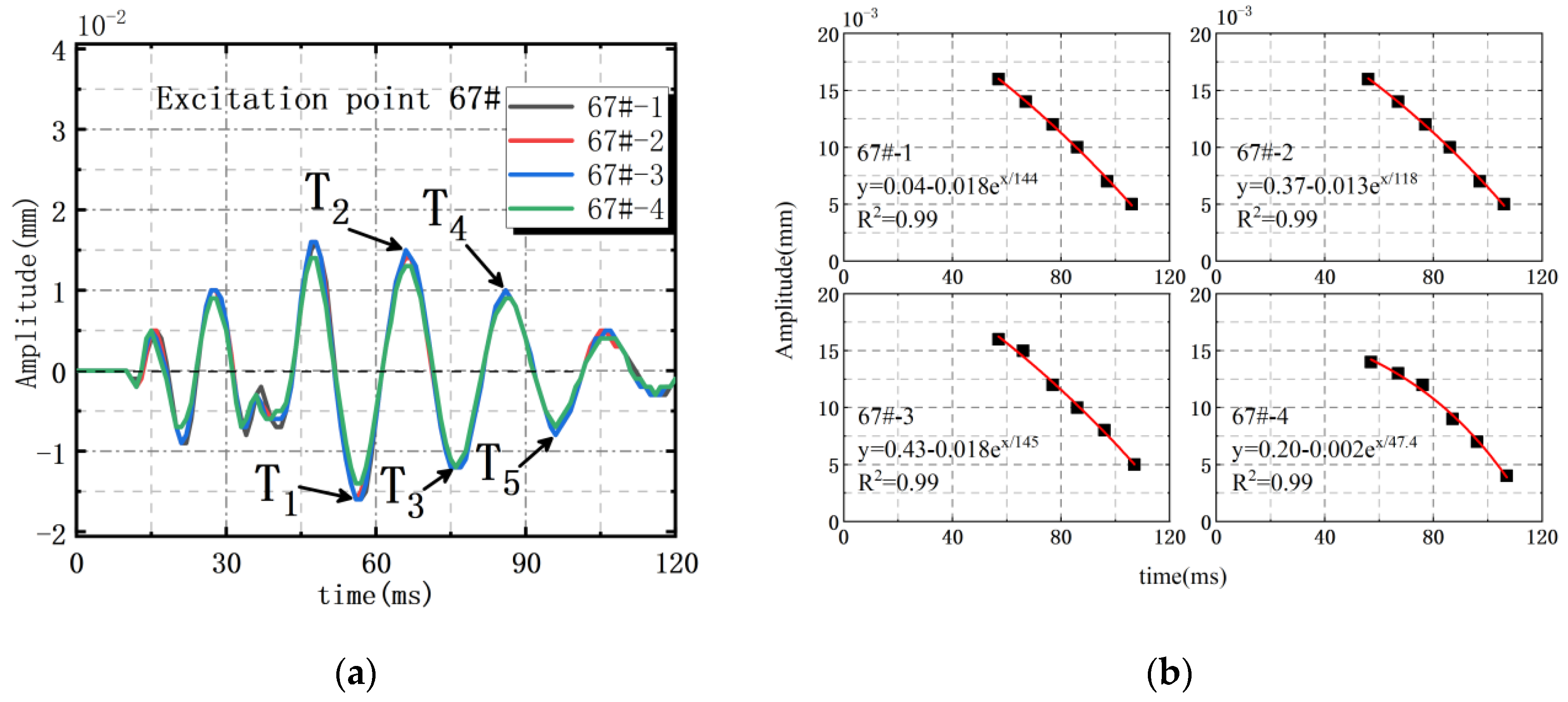
3.2.2. Dynamic Attenuation Law of Amplitude under Multi-Point Excitation

The analysis results of the amplitude extreme value under multi–point excitation showed that the dynamic changes were similar. The extreme values distribution of the test curves when 6# and 7# action points were excited synchronously can be seen in

Table 5. Amplitude extreme points of No. 1–4 under 6# and 7# action points excited synchronously.

Extreme Point	Time (ms)	No. 1 (mm)	Time (ms)	No. 2 (mm)	Time (ms)	No. 3 (mm)	Time (ms)
T1	57	0.016	56	0.016	57	0.016	57
T2	67	0.014	67	0.014	66	0.015	67
T3	77	0.012	77	0.012	77	0.012	76
T4	86	0.01	86	0.01	86	0.01	87
T5	97	0.007	97	0.007	96	0.008	96

, and the curve–fitting results are shown in Figure 9. It could be concluded that the dynamic attenuation of amplitude under single point excitation also conformed to the law of exponential variation y = y0 + Aexp (x/k), and the fitting degree was as high as 0.99.

4. Amplitude-Frequency Distribution of Interface Vibration under Impact Load

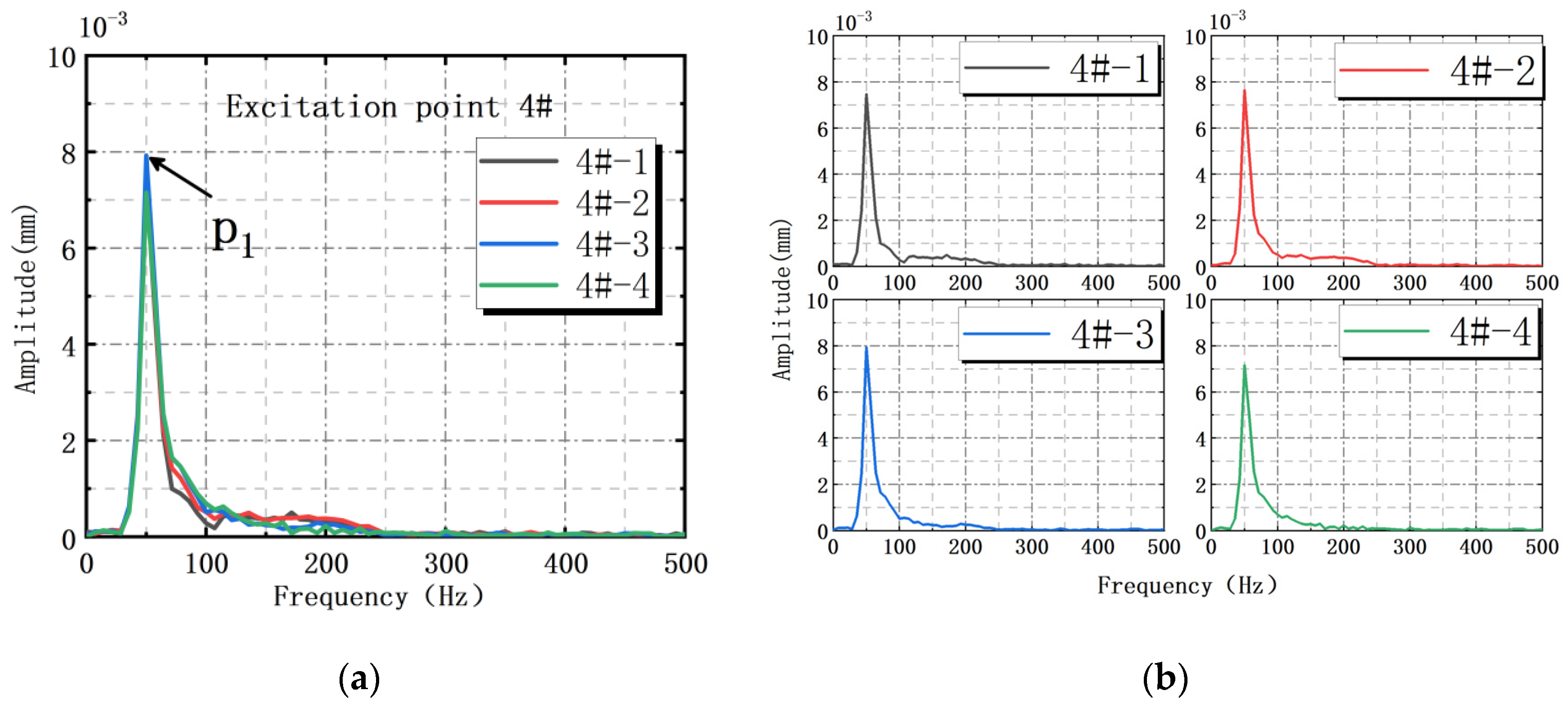
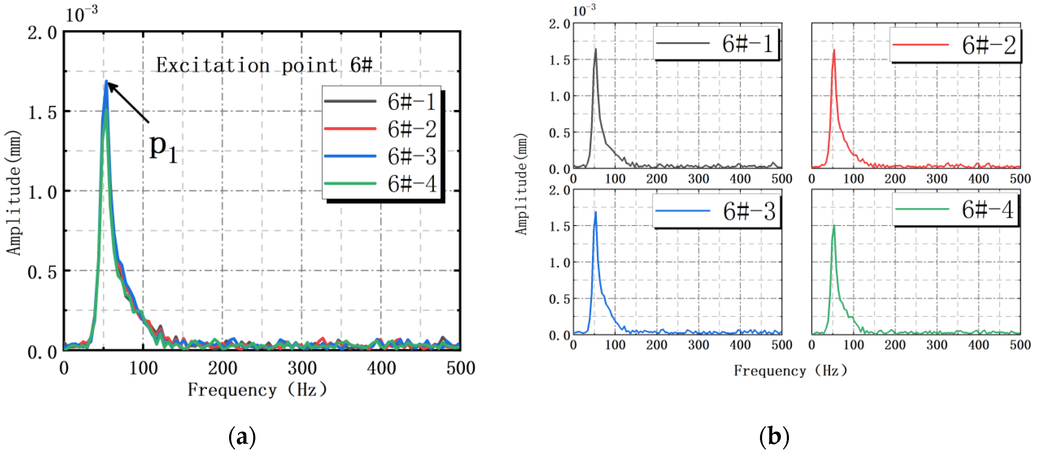
4.1. Amplitude-Frequency Distribution of Interface Vibration under Single Point Excitation

The amplitude–frequency distributions when the 2#, 4# and 6# action points were excited separately are shown in Figure 10, Figure 11 and Figure 12. When the 2# action point was excited, the amplitude of No. 1 (2#-1 in Figure 10) reached the peak 7.2 × 10⁻³ mm at P₁ = 50 Hz. When the 4# action point was excited, the amplitude of No. 1 (4#-1 in Figure 11) reached the peak 7.5 × 10⁻³ mm at P₁ = 50 Hz. When the 6# action point was excited, the amplitude of No. 1 (6#-1 in Figure 12) reached the peak 1.6 × 10⁻³ mm at P₁ = 53.7 Hz. The amplitude variations of No. 2~4 were all similar to that of No. 1.

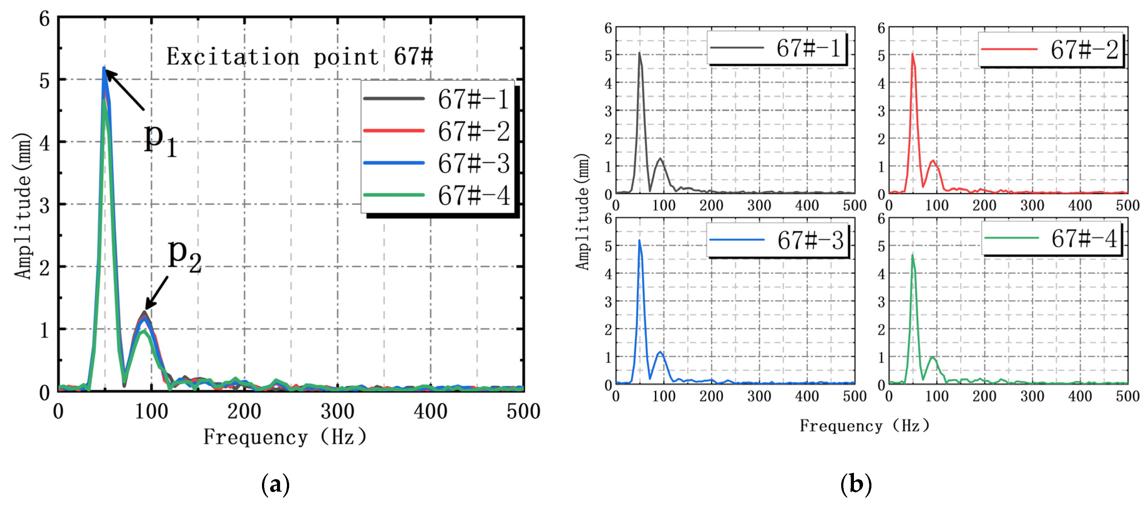
4.2. Amplitude-Frequency Distribution under Multi-Point Excitation Step-by-Step

The amplitude–frequency distributions when 2# and 4# action points were excited step-by-step are shown in Figure 13. The amplitude of No. 1 (24#-1 in Figure 13) reached the peak 5.4 × 10⁻³ mm at P₁ = 52.1 Hz, compared with single point excitation, the vibration complexity of multi-point excitation step-by-step was relatively high, and the amplitude variations of No. 2~4 were all similar to that of No. 1.

4.3. Amplitude-Frequency Distribution under Multi-Point Synchronous Excitation

The amplitude–frequency distributions when 2# and 4# action points were excited synchronously are shown in Figure 14. The amplitude of No. 1 (67#-1 in Figure 14) reached the peak 5.1 × 10⁻³ mm at P₁ = 48.9 Hz, the second peak 1.3 × 10⁻³ mm at P₂ = 92.4 Hz, and the amplitude variations of No. 2~4 were all similar to that of No. 1.

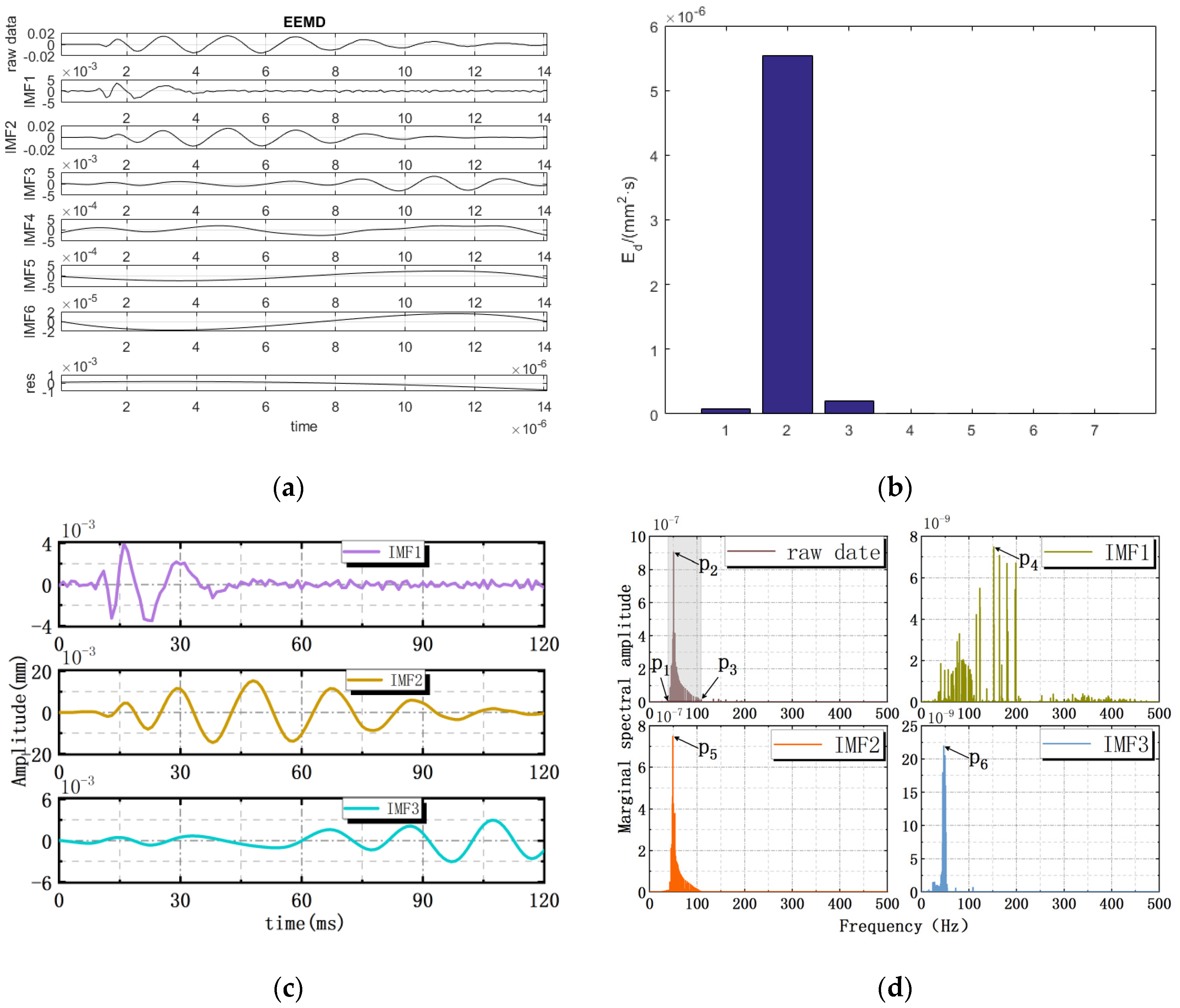
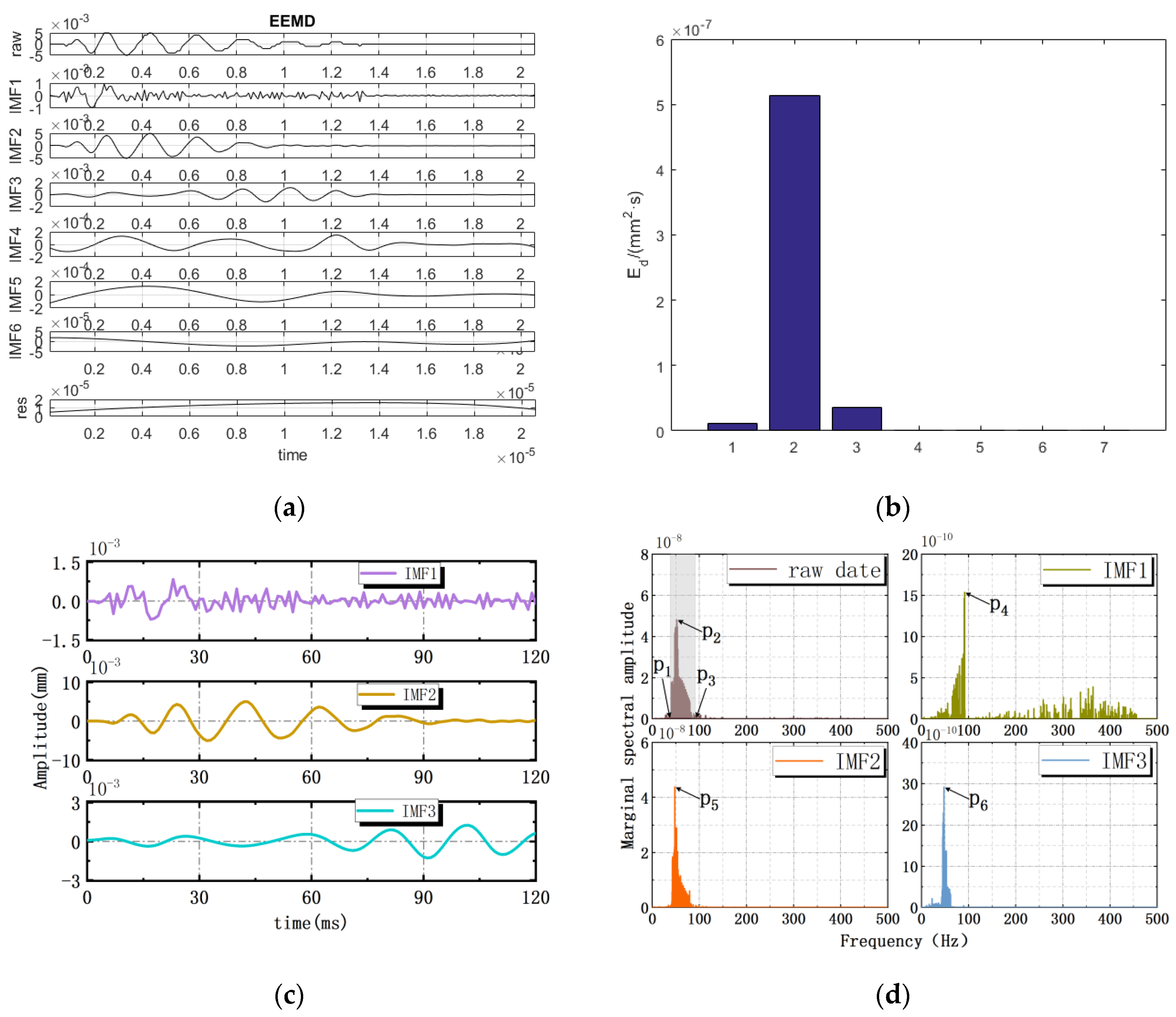
5. Effective Vibration Modes and Predominant Frequency of Interface Vibration under Impact Load

Based on Hilbert Huang transform (HHT), the interface vibration waveforms were decomposed by EEMD [20,21,22,23,24]; combined with energy formula: ${\int }_{-\infty }^{\infty }{\mathrm{x}}^2\left(\mathrm{t}\right)\mathrm{dt}$, the energy distributions and marginal spectrum of the decomposed waveforms were obtained [25].

Under 2# action point excitation, the decomposition result of the vibration waveform is shown in Figure 15, which was decomposed into five vibration modes (IMF1~IMF5), and the residual res <10⁻³ (Figure 15a). The energy proportions of modes IMF1, IMF2 and IMF3 were relatively high (Figure 15b), which were the effective vibration modes. Among them, the energy proportion of IMF2 was the highest, accounting for about 96% of the total energy, which was the main vibration mode. By analyzing the marginal spectrum of the original waveform and effective vibration modes (Figure 15c,d), it could be concluded that the vibration frequency of the original waveform was mainly concentrated in P₁~P₃ = 39.9~89.8 Hz, and the predominant frequency corresponding to the peak was P₂ = 52.9 Hz. The predominant frequencies of effective vibration modes (IMF1, IMF2 and IMF3) were P₄ = 236.8 Hz, P₅ = 50.2 Hz and P₆ = 35.9 Hz respectively.

Under 4# action point excitation, the decomposition result of vibration waveform are shown in Figure 16, which was decomposed into six vibration modes (IMF1~IMF6), and the residual res <10⁻³ (Figure 16a). The energy proportions of modes IMF1, IMF2 and IMF3 were relatively high (Figure 16b), which were the effective vibration mode. Among them, the energy proportion of IMF2 was the highest, accounting for about 95% of the total energy, which was the main vibration mode. By analyzing the marginal spectrum of the original waveform and effective vibration modes (Figure 16c,d), it could be concluded that the vibration frequency of the original waveform was mainly concentrated in P₁~P₃ = 38.9~108.8 Hz, and the predominant frequency corresponding to the peak was P₂ = 50.4 Hz. The predominant frequencies of effective vibration modes (IMF1, IMF2 and IMF3) were P₄ = 152.4 Hz, P₅ = 49.2 Hz and P₆ = 47 Hz respectively.

Under 6# action point excitation, the decomposition result of vibration waveform was shown in Figure 17, which was decomposed into six vibration modes (IMF1~IMF6), and the residual res <10⁻³ (Figure 17a). The energy proportions of modes IMF1, IMF2 and IMF3 were relatively high (Figure 17b), which were the effective vibration modes. Among them, the energy proportion of IMF2 was the highest, accounting for about 92% of the total energy, which was the main vibration mode. By analyzing the marginal spectrum of the original waveform and effective vibration modes (Figure 17c,d), it could be concluded that the vibration frequency of the original waveform was mainly concentrated in P₁~P₃ = 37.8~92.7 Hz, and the predominant frequency corresponding to the peak was P₂ = 52.3 Hz. The predominant frequencies of effective vibration modes (IMF1, IMF2 and IMF3) were P₄ = 91.3 Hz, P₅ = 47.7 Hz and P₆ = 47.7 Hz respectively.

Under 2# and 4# action points excitation step-by-step, the decomposition result of the vibration waveform is shown in Figure 18, which was decomposed into seven vibration modes (IMF1~IMF7), and the residual res <10⁻⁴ (Figure 18a). The energy proportions of modes IMF1, IMF2 and IMF3 were relatively high (Figure 18b), which were the effective vibration mode. Among them, the energy proportion of IMF2 was the highest, accounting for about 86% of the total energy, which was the main vibration mode. By analyzing the marginal spectrum of the original waveform and effective vibration modes (Figure 18c,d), it could be concluded that the vibration frequency of the original waveform was mainly concentrated in P₁~P₃ = 37.5~99.9 Hz, and the predominant frequency corresponding to the peak was P₂ = 49.4 Hz. The predominant frequencies of effective vibration modes (IMF1, IMF2 and IMF3) were P₄ = 82.7 Hz, P₅ = 48.6 Hz and P₆ = 46.5 Hz, respectively.

Under 6# and 7# action points synchronous excitation, the decomposition result of vibration waveform was shown in Figure 19, which was decomposed into six vibration modes (IMF1~IMF6), and the residual res <10⁻³ (Figure 19a). The energy proportions of modes IMF1, IMF2 and IMF3 were relatively high (Figure 19b), which were the effective vibration modes. Among them, the energy proportion of IMF2 was the highest, accounting for about 85% of the total energy, which was the main vibration mode. By analyzing the marginal spectrum of the original waveform and the effective vibration modes (Figure 19c,d), it could be concluded that the vibration frequency of the original waveform was mainly concentrated in P₁~P₃ = 24.8~90.2 Hz, and the predominant frequency corresponding to the peak was P₂ = 45.7 Hz. The predominant frequencies of effective vibration modes (IMF1, IMF2 and IMF3) were P₄ = 201.3 Hz, P₅ = 45.6 Hz and P₆ = 47.4 Hz, respectively.

It could be seen that IMF1, IMF2 and IMF3 were effective vibration modes under single point excitation and multi-point excitation (synchronous/step-by-step). Among them, the energy of IMF2 accounted for the highest proportion (85–94%), which was the main vibration mode, and its predominant frequencies were mostly concentrated in 45.6~50.2 Hz. It could be concluded that IMF2 played a decisive role in the vibration process, so the predominant frequencies of coal–rock and rock–rock interfaces vibration under impact load were also concentrated in this range, and the vibration in this frequency range had an important effect on the dynamic response, damage and failure of coal and rock mass. Of course, in the actual conditions, the range of the actual predominant frequencies could be obtained by converting according to the size and mechanical properties of coal and rock mass.

6. Conclusions

Under single and multi–point excitation (synchronous/step-by-step), the dynamic changes of amplitude curves of each interface vibration were obtained from the four sensors (No. 1~4) were similar, and the extreme value showed two stages as follows: first increase and then attenuation, most of which required 2.25 cycles to reach the peak. The dynamic attenuation of amplitude conformed to the law of exponential variation y = y0 + Aexp (x/k).

Based on FFT transform, the time–history curves of interface vibration under single point and multi-point excitation (synchronous/step-by-step) were analyzed, and the predominant frequencies distribution of amplitude were obtained. Among them, the two predominant frequencies were P₁ = 48.9~53.7 Hz and P₂ = 92.4 Hz.

The time–history curves of interface vibration under single point and multi-point excitation (synchronous/step-by-step) were decomposed by EEMD to obtain a total of 5~7 component modes (IMF), of which IMF1, IMF2 and IMF3 contained high energy and were effective vibration modes.

The energy of IMF2 accounted for the highest proportion (85–94%), which was the main vibration mode, and its predominant frequencies were concentrated in 45.6~50.2 Hz, which overlapped with that of the original waveform to a great extent. The vibration of IMF2 played a decisive role in the vibration process and had an important effect on the dynamic response, damage, and failure of coal and rock mass. In actual conditions, the range of the actual predominant frequencies can be obtained by converting according to the size and mechanical properties of coal and rock mass.

In this paper, the characteristics of vibration frequency and vibration amplitude of coal rock vibration response signal were mainly studied. The vibration frequency study of coal rock vibration signals can help the monitoring and early warning of coal and gas protrusion. The study of vibration amplitude can help to determine the danger area of coal rock vibration. The vibration frequency characteristics and amplitude characteristics of the dynamic response signals of coal rocks have rarely been studied by previous authors; there are even fewer studies on the dynamic response characteristics of multi-layer coal rocks. In this paper, we studied the dynamic response characteristics of the five–seam coal rock body, which is closer to the complex reality. However, the study only performs vibration response analysis for similar experiments in this paper. Further studies are needed to verify whether the dynamic response of coal rock in different scenarios also conforms to the vibration law summarized in this study. Further research is needed to investigate the dynamic response of coal rocks under different sizes and mechanical properties of the actual site.

References

1. Xu, D.P.; Feng, X.T.; Chen, D.F.; Zhang, C.Q.; Fan, Q.X. Constitutive representation and damage degree index for the layered rock mass excavation response in underground openings. Tunn. Undergr. Space Technol. 2017, 64, 133–145. [Google Scholar] [CrossRef]
2. Wang, P.T.; Cai, M.F.; Ren, F.H. Anisotropy and directionality of tensile behaviours of a jointed rock mass subjected to numerical Brazilian tests. Tunn. Undergr. Space Technol. 2018, 64, 133–145. [Google Scholar] [CrossRef]
3. Liu, Y.S.; He, C.S.; Fu, H.L.; Wang, S.M.; Lei, Y.; Peng, Y.X. Study on dynamic and static mechanical properties and failure mode of layered slate. J. Railw. Sci. Eng. 2020, 17, 2789–2797. [Google Scholar] [CrossRef]
4. Wu, G.P.; Shen, W.W.; Cui, K.; Wang, P. Degradation behavior and mechanism of slate under alternating conditions of freeze-thaw and wet-dry. J. Cent. South Univ. (Sci. Technol.) 2019, 50, 92–1402. [Google Scholar] [CrossRef]
5. Liu, Y.S.; Wang, S.M.; Yan, S.J.; Fu, H.L.; Chen, C.; Shi, Y.; Yue, J. Properties and failure mechanism of layered sandstone based on acoustic emission experiments. J. Cent. South Univ. (Sci. Technol.) 2019, 50, 1419–1427. [Google Scholar] [CrossRef]
6. Zhou, P.F.; Shen, Y.S.; Zhao, J.F.; Zhang, X.; Gao, B.; Zhu, S.Y. Research on disaster-induced mechanism of tunnels with steeply dipping phyllite strata based on an improved ubiquitous-joint constitutive model. Chin. J. Rock Mech. Eng. 2019, 38, 1870–1883. [Google Scholar] [CrossRef]
7. Su, G.S.; Hu, L.H.; Feng, X.T.; Wang, J.H.; Zhang, X.H. True triaxial experimental study of rockburst process under low frequency cyclic disturbance load combined with static load. Chin. J. Rock Mech. Eng. 2016, 35, 1309–1322. [Google Scholar] [CrossRef]
8. Chang, W.B.; Fan, S.W.; Zhang, L.; Shu, L.Y. A model based on explosive stress wave and tectonic coal zone which gestate dangerous state of coal and gas outburst. J. China Coal Soc. 2014, 39, 2226–2231. [Google Scholar] [CrossRef]
9. Zuo, J.P.; Chen, Y.; Cui, F. Investigation on mechanical properties and rock burst tendency of different coal-rock combined bodies. J. China Univ. Min. Technol. 2018, 47, 81–87. [Google Scholar] [CrossRef]
10. Li, S.H.; Zhu, W.C.; Niu, L.L.; Yu, M.; Chen, C.F. Dynamic characteristics of green sandstone subjected to repetitive impact loading: Phenomena and mechanisms. Rock Mech. Rock Eng. 2018, 51, 1921–1936. [Google Scholar] [CrossRef]
11. Mu, Z.L.; Wang, H.; Peng, P.; Liu, Z.J.; Yang, X.C. Experimental research on failure characteristics and bursting liability of rock-coal-rock sample. J. Min. Saf. Eng. 2013, 30, 841–847. [Google Scholar]
12. Liu, S.H.; Qin, Z.H.; Lou, J.F. Experimental study of dynamic failure characteristics of coal-rock compound under one-dimensional static and dynamic loads. Chin. J. Rock Mech. Eng. 2014, 33, 2064–2075. [Google Scholar] [CrossRef]
13. Potvin, Y.; Hadjigeorgiou, J.; Stacey, D. Challenges in Deep and High Stress Mining; Australian Center for Geomechanics: Nedlands, Australia, 2007. [Google Scholar]
14. Hoke, E. Progressive caving induced by mining an inclined orebody. Trans. Inst. Min. Metall. 1974, 83, 133–139. [Google Scholar]
15. Braunagel, M.J.; Griffith, W.A. The effect of dynamic stress cycling on the compressive strength of rocks. Geophys. Res. Lett. 2019, 46, 6479–6486. [Google Scholar] [CrossRef]
16. Cui, F.; Yang, Y.B.; Lai, X.P.; Cao, J.T. Similar material simulation experimental study on rockbursts induced by key stratum breaking based on microseismic monitoring. Chin. J. Rock Mech. Eng. 2019, 38, 803–814. [Google Scholar] [CrossRef]
17. Li, F.; Dong, X.H.; Wang, Y.; Liu, H.W.; Chen, C.; Zhao, X. The Dynamic Response and Failure Model of Thin Plate Rock Mass under Impact Load. Shock. Vib. 2021, 2021, 9998558. [Google Scholar] [CrossRef]
18. Yang, S.L.; Wang, J.C.; Yang, J.H. Physical analog simulation analysis and its mechanical explanation on dynamic load impact. J. China Coal Soc. 2017, 42, 335–343. [Google Scholar] [CrossRef]
19. Song, X.L.; Gao, W.X.; Ji, J.M.; Ye, M.B.; Zhang, D.J. Blasting damage analysis method based on EEMD-HHT transform. J. Cent. South Univ. (Sci. Technol.) 2017, 42, 335–343. [Google Scholar] [CrossRef]
20. Zhao, Y.; Shan, R.L.; Wang, H.L. Research on vibration effect of tunnel blasting based on an improved Hilbert–Huang transform. Environ. Earth Sci. 2021, 80, 206. [Google Scholar] [CrossRef]
21. Hamdi, S.E.; Le, D.A.; Simon, L.; Plantier, G.; Sourice, A.; Feuilloy, M. Acoustic emission pattern recognition approach based on Hilbert–Huang transform for structural health monitoring in polymer-composite materials. Appl. Acoust. 2013, 74, 746–757. [Google Scholar] [CrossRef]
22. Liu, X.; Wang, J.; Li, W. A time-frequency extraction model of structural vibration combining VMD and HHT. Geomat. Inf. Sci. Wuhan Univ. 2021, 46, 1686–1692. [Google Scholar] [CrossRef]
23. Dragomiretskiy, K.; Zosso, D. Variational Mode Decomposition. IEEE Trans. Signal Process. 2014, 62, 531–544. [Google Scholar] [CrossRef]
24. Lu, C.P.; Dou, L.M.; Wu, X.R.; Mou, Z.L.; Chen, G.X. Experimental and Empirical Research on Frequency-Spectrum Evolvement Rule of Rockburst Precursory Microseismic Signals of Coal-Rock. Chin. J. Rock Mech. Eng. 2008, 27, 519–525. [Google Scholar] [CrossRef]
25. Zhang, P.S.; Liu, S.D. The Structure Character of Coal and Rock by Seismic Wave Spectrum Analyzing Technology and Its Application. Chin. J. Eng. Geophys. 2006, 3, 274–277. [Google Scholar] [CrossRef]
Figure 1. Experimental model and data acquisition system.
Processes 11 00306 g001
Figure 2. Action points and sensors distribution in combined coal and rock mass.
Processes 11 00306 g002
Figure 3. Amplitude time–history curves under 2# action point excited alone. (a) Overlapping display of the four sensor signals; (b) Separate display of the four sensor signals.
Processes 11 00306 g003
Figure 4. Amplitude time–history curves under 4# action point excited alone. (a) Overlapping display of the four sensor signals; (b) Separate display of the four sensor signals.
Processes 11 00306 g004
Figure 5. Amplitude time-history curves under 6# action point excited alone. (a) Overlapping display of the four sensor signals; (b) Separate display of the four sensor signals.
Processes 11 00306 g005
Figure 6. Amplitude time-history curves under 2# and 4# action points excited step by step. (a) Overlapping display of the four sensor signals; (b) Separate display of the four sensor signals.
Processes 11 00306 g006
Figure 7. Amplitude time-history curves under 6# and 7# action points excited synchronously. (a) Overlapping display of the four sensor signals; (b) Separate display of the four sensor signals.
Processes 11 00306 g007
Figure 8. Amplitude attenuation law under 2# action point excitation. (a) Overlapping display of the four sensor signals; (b) Curve-fitting results of curve decay extreme value.
Processes 11 00306 g008
Figure 9. Amplitude attenuation law under 6# and 7# action points excited synchronously. (a) Overlapping display of the four sensor signals; (b) Curve-fitting results of curve decay extreme value.
Processes 11 00306 g009
Figure 10. Amplitude–frequency distribution of interface vibration under 2# action point excitation. (a) Overlapping display of the four sensor signals; (b) Separate display of the four sensor signals.
Processes 11 00306 g010
Figure 11. Amplitude–frequency distribution of interface vibration under 4# action point excitation. (a) Overlapping display of the four sensor signals; (b) Separate display of the four sensor signals.
Processes 11 00306 g011
Figure 12. Amplitude–frequency distribution of interface vibration under 6# action point excitation. (a) Overlapping display of the four sensor signals; (b) Separate display of the four sensor signals.
Processes 11 00306 g012
Figure 13. Amplitude–frequency distribution under 2# and 4# action points excited step-by-step. (a) Overlapping display of the four sensor signals; (b) Separate display of the four sensor signals.
Processes 11 00306 g013
Figure 14. Amplitude–frequency distribution under 6# and 7# action points excited synchronously. (a) Overlapping display of the four sensor signals; (b) Separate display of the four sensor signals.
Processes 11 00306 g014
Figure 15. The waveform decomposition under 2# action point excitation. (a) The EEMD decomposition of the interface vibration waveform; (b) Energy distribution of the decomposed waveform; (c) Effective vibration modes; (d) Marginal spectral amplitude.
Processes 11 00306 g015
Figure 16. The waveform decomposition under 4# action point excitation. (a) The EEMD decomposition of the interface vibration waveform; (b) Energy distribution of the decomposed waveform; (c) Effective vibration modes; (d) Marginal spectral amplitude.
Processes 11 00306 g016
Figure 17. The waveform decomposition under 6# action point excitation. (a) The EEMD decomposition of the interface vibration waveform; (b) Energy distribution of the decomposed waveform; (c) Effective vibration modes; (d) Marginal spectral amplitude.
Processes 11 00306 g017
Figure 18. The waveform decomposition under 2# and 4# action points excited step-by-step. (a) The EEMD decomposition of the interface vibration waveform; (b) Energy distribution of the decomposed waveform; (c) Effective vibration modes; (d) Marginal spectral amplitude.
Processes 11 00306 g018
Figure 19. The waveform decomposition under 6# and 7# action points excited synchronously. (a) The EEMD decomposition of the interface vibration waveform; (b) Energy distribution of the decomposed waveform; (c) Effective vibration modes; (d) Marginal spectral amplitude.
Processes 11 00306 g019