Magneto-Thermal Coupling Simulation of Flowing Liquid Induction Heating through Static Mixer-Type Susceptors

Abstract

As a new non-contact heating technology, induction heating technology has very broad application prospects in the field of fluid food heating. However, its application is inevitably affected by the heat concentration caused by uneven energy distribution. The uneven temperature distribution of the heating process will lead to the decrease in the quality of heating products. Therefore, based on the previous research, in order to improve the uniformity of heat distribution in the heating process, this study selected the susceptor with the greatest potential for efficient and the most uniform heating fluid to carry out the coupling simulation of electromagnetic heat transfer. The susceptor was simulated and optimized in three aspects: different power comparisons, the influence of structural change on temperature distribution uniformity, and the influence of physical property change of metal material on temperature distribution uniformity. The results show that the simulation results are in good agreement with the experimental results, and the error between the experimental and simulation values of the outlet temperature at Kelvin temperature is less than 0.18%. The change of geometric structure had a great influence on the uniformity of temperature distribution, and the uniformity of temperature distribution was inversely proportional to the conductivity. During the simulation, the temperature of the fluid heated by the susceptor was increased from 284.75 K to about 333K. The temperature distribution of the fluid at the outlet of the susceptor was uniform, and the temperature difference was about 1 K.

1. Introduction

Induction heating is a new heating technology that uses alternating magnetic fields to generate eddy currents in the heated workpiece to heat the workpiece. It has the advantages of high efficiency, energy efficiency, and easy control [1]. Based on the high efficiency and energy-saving advantages of induction heating technology, scholars began to study the application of induction heating technology in the liquid food processing industry [2,3]. However, uneven temperature distribution in the process of heating flowing liquid is a problem with induction heating technology.

In previous studies, the conductive structure used for heating the flowing liquid was collectively referred to as the susceptor. There are four kinds of susceptors: metal pipe susceptor, metal sphere susceptor, sheet metal susceptor, and static mixer-type susceptor [4]. Previously, some scholars have carried out some applied research on metal pipe susceptors [2,5,6]. However, due to the shielding effect of the outer wall of the metal pipe susceptor on the internal cavity, the internal components cannot be heated normally, and it is difficult to heat evenly [7]. The metal sphere susceptor can achieve uniform heating by dispersing the heated fluid in a fixed or moving form [8,9,10]. However, the heating efficiency of this kind of susceptor in previous studies was low. In summary, among the four susceptors studied previously, the static mixer-type susceptor has the potential to uniformly heat fluid while ensuring high heating efficiency, but the structure still needs to be optimized. Therefore, this paper further optimizes the static mixer-type susceptor by means of simulation analysis.

At present, some scholars have studied the process of fluid induction heating under forced flow or non-forced flow. In 2020, Kilic et al. [11] designed an immersed thin-walled cylinder heater based on induction heating for liquid heating and verified the influence of the geometry of the susceptor on the temperature distribution uniformity of the heating process. Icier et al. [12] used COMSOL MultiPhysical software to simulate the continuous induction heating process of sour cherry juice. The influence of the process’s parameters on its heating effect was studied. Kawakami et al. [13] carried out CFD analysis on induction heating and gas heating in metal pots. The heat generation distribution was obtained as the boundary condition by electromagnetic field analysis. The temperature distribution and velocity distribution of the fluid in the induction heating process under the non-forced flow state were analyzed by computational fluid dynamics. Kastillo et al. [14] also conducted a similar analysis of the heating process of olive oil in containers made of aluminum, enameled iron, and stainless steel. The mentioned research either used simulation to optimize the device or used simulation to study the heat transfer process. However, these simulations did not fully study the influence of changes in the physical parameters of the susceptor material on the induction heating process.

Generally, when the temperature of metal material changes greatly, it tends to follow the temperature change in the conductive structure when the material properties change with temperature by means of magneto-thermal two-way coupling. For example, Eom et al. [15] and Chang et al. [16] considered the change of physical parameters with temperature in the process of induction injection molding. In the case of heat exchange between heated metal and gas, it was more necessary to consider the change of material properties with temperature (Kranjc et al. [17] Jang et al. [18]). However, in general, such two-way coupling needs to consume a lot of computing resources; thus, some scholars use the interval value method to study changes in physical parameters. For example, Bio et al. [19] studied the induction heating process by selecting different levels of conductivity and permeability values. However, in general, only by comprehensively considering temperature-dependent parameters such as thermal conductivity and electrical conductivity can one obtain the most realistic results.

In summary, the technology of numerical analysis of the induction heating process with finite element software such as Ansys is mostly used to analyze changes in solid- or fluid-state parameters during induction heating. The purpose of this study is to improve the uniformity of temperature distribution during the heating process of flowing liquid materials with induction heating technology. In this study, the static mixer-type susceptor proposed in a previous study, which has the most potential for the efficient and uniform heating of fluids, was taken as the research object [4]. The numerical analysis method was used to study the state parameters of the static mixer-type susceptor in the process of fluid heating under forced convection heat transfer in three aspects: heating power, geometric structure, and the material parameters of the susceptor. On this basis, the susceptor was optimized, and the influence of material parameters on the heating process was considered.

2. Simulation Methods

2.1. Simulation Model Establishment

2.1.1. Governing Equations

When an alternating current with a certain frequency is introduced into the induction coil, an alternating magnetic field with a certain frequency will be generated inside and around the induction coil, which is the basis for the metal parts in the induction coil to be heated by induction. The distribution of electromagnetic field can be expressed by Maxwell’s Equation (1) and Auxiliary Equation (2) [15,16], which are composed of the Ampere circuit theorem, Faraday’s law of electromagnetic induction, Gauss flux, and magnetic flux law. In the simulation process, these equations, using Maxwell as the default, were as follows:

$$\left\{\begin{array}{c}\begin{array}{c}\nabla \times \overline{\mathrm{H}}=\overline{\mathrm{J}}+\frac{\partial \overline{\mathrm{D}}}{\partial \mathrm{t}}\\ \nabla \times \overline{\mathrm{E}}=-\frac{\partial \overline{\mathrm{B}}}{\partial \mathrm{t}}\end{array}\\ \begin{array}{c}\nabla ·\overline{\mathrm{D}}=\mathsf{\rho }\\ \nabla ·\overline{\mathrm{B}}=0\end{array}\end{array}\right.$$

(1)

$$\left\{\begin{array}{c}\overline{\mathrm{D}}=\mathsf{\epsilon }\overline{\mathrm{E}}\\ \overline{\mathrm{J}}=\mathsf{\sigma }\overline{\mathrm{E}}=\frac{\overline{\mathrm{E}}}{\mathsf{\rho }}\\ \overline{\mathrm{B}}=\mathsf{\mu }\overline{\mathrm{H}}\end{array}\right.$$

(2)

where $\overline{\mathrm{H}}$ is the magnetic field’s strength (A/m); $\overline{\mathrm{J}}$ is the current density (A/m²); $\overline{\mathrm{D}}$ is the electric flux density (C/m²); ρ is the charge density (C/m³); $\overline{\mathrm{E}}$ is the electric field intensity (V/m); $\overline{\mathrm{B}}$ is the magnetic flux density (Wb/m²); $\mathsf{\mu }$ is the permeability (H/m); $\mathsf{\sigma }$ is the electrical conductivity (S/m); $\mathsf{\epsilon }$ is the dielectric constant (F/m).

In the fluid simulation stage, the pressure–velocity coupling adopted the SIMPLE algorithm, and the energy equation and momentum equation adopted the system’s default first-order upwind algorithm. The continuity, momentum, and energy calculation process was performed to meet the following relationship [20]:

Continuity equation:

$$\nabla \mathrm{U}=0$$

(3)

Momentum equation:

$$\mathsf{\rho }\frac{\mathrm{DU}}{\mathrm{Dt}}=-\nabla \mathrm{p}+{\nabla }^2\mathsf{\mu }\mathrm{U}+\mathsf{\rho }\mathrm{g}$$

(4)

Energy equation:

$${\mathsf{\rho }\mathrm{C}}_{\mathrm{p}}\frac{\mathrm{DT}}{\mathrm{Dt}}=\mathsf{\lambda }{\nabla }^2\mathrm{T}+\mathsf{\mu }\dot{\mathsf{\gamma }}{ }^2$$

(5)

where p is the fluid pressure (Pa); g is the gravitational acceleration (m/s²); $\mathsf{\rho }$ is the fluid density (kg/m³); $\mathsf{\mu }$ is the viscosity (Pa·s); ${\mathrm{C}}_{\mathrm{p}}$ is the constant pressure specific heat capacity (J/(kg·K)); $\mathsf{\lambda }$ is the thermal conductivity of fluids (w/(m·K)); T is the flow temperature K; U is the velocity field (m/s); $\dot{\mathsf{\gamma }}$ is the second invariant of the shear rate tensor, which is defined as $(\dot{\mathsf{\gamma }}=[\frac{1}{2}(\dot{\mathsf{\gamma }}:\dot{\mathsf{\gamma }}){]}^{\frac{1}{2}})$.

2.1.2. Susceptor, Coil, and Fluid Domain Structure

Before the simulation analysis, the static mixer-type susceptor was modeled. The geometric model obtained from modeling can be divided into three parts: the static mixer-type susceptor, the induction heating coil, and the fluid domain.

The first part is the susceptor part. In the experiment, the metal plates in the static mixer-type susceptor were connected and limited by the screw rod and the nylon foot column, but it was difficult to mesh the complex and small gap in the simulation process. Therefore, in order to simplify the model and reduce the amount of calculation, the connectors and connecting holes between the metal plates of the susceptor were neglected in the modeling process. Two intersecting metal plates were one group, and the thickness of the metal plates was 0.5 mm. The geometric relationship between the two groups is shown in Figure 1a. The geometric structure of each metal plate is shown in Figure 1b.

The second part is the coil part. The induction heating coil used in the simulation process was modeled exactly as the coil used in the experiment. The copper coil had the following parameters: 10 turns, spacing of 20 mm, coil diameter of 76 mm, copper tube outside diameter of 8 mm, and wall thickness of 1 mm. The model is shown in Figure 1c.

Finally, in the fluid domain part in the modeling process, the quartz tube wall located outside the susceptor was not modeled for the consideration of drawing the grid, and the limitation of the fluid flow range was realized with subsequent fluid domain modeling. The diameter of the fluid domain was 60 mm in accordance with the inner diameter of the quartz tube during the experiment. In addition, because the induction heating coil was not involved in the fluid–solid coupling heat transfer, the induction heating coil was separated in the fluid domain modeling stage. The final model is shown in Figure 1d.

In the simulation process, two different geometric structures, one with a 10° cross angle and another with a 15° cross angle, were selected for analysis. The 10° cross angle susceptor had 78 metal plates, and the 15° cross angle susceptor had 52 metal plates. The combination of the two susceptors was the same as the geometric structure of a single metal plate. Thus, only the geometry of the 10° cross angle susceptor is shown here.

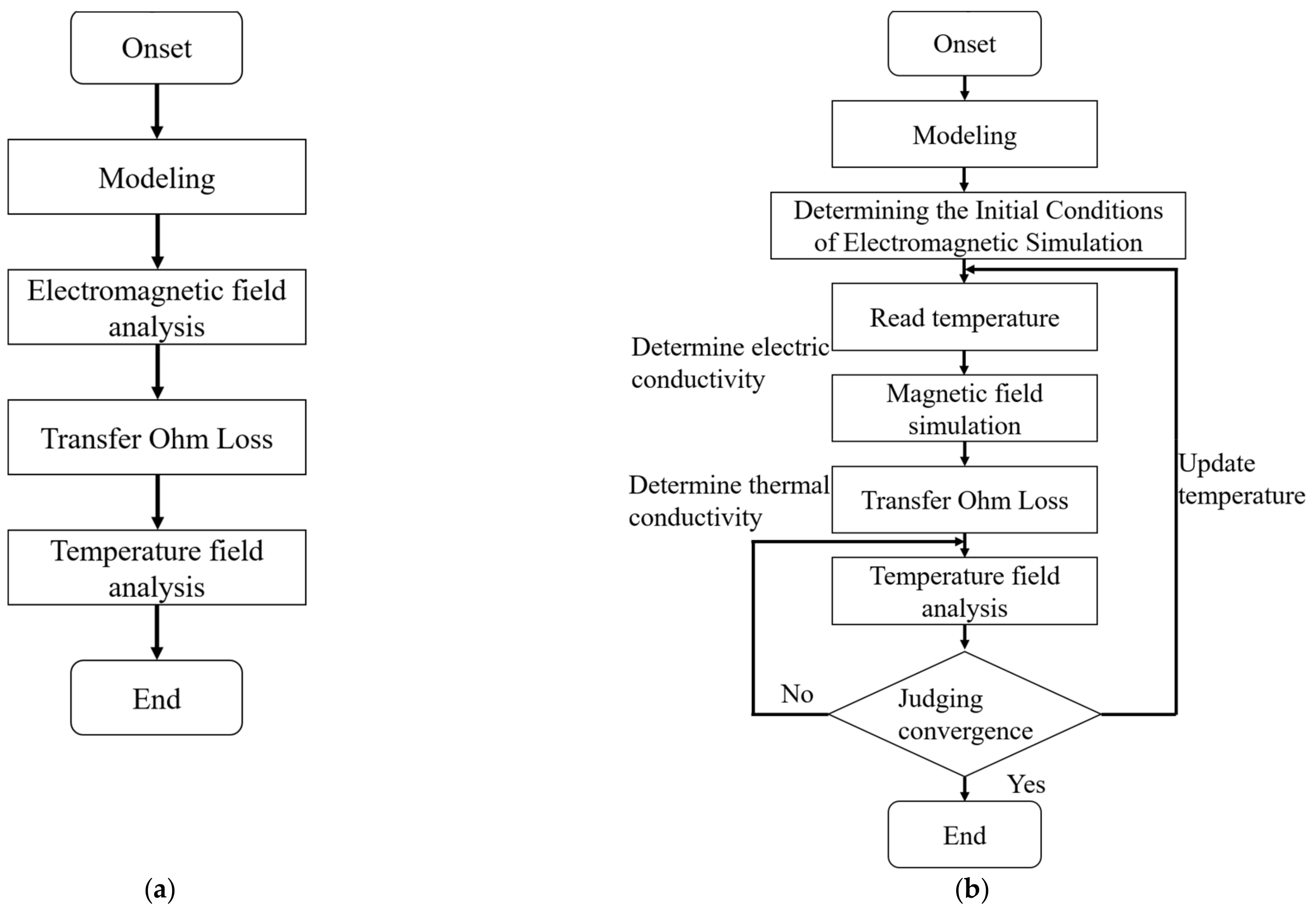
2.1.3. Selection of Physical Parameters and Simulation Process

The coil material was copper, and the coil parameters were set with reference to the copper parameters in the Maxwell material library. The susceptor material selection was 304 stainless steel, but because the software material library did not contain 304 stainless steel, the relevant literature was referenced for 304 stainless steel’s material properties. The physical parameters are summarized in

Table 1. Physical parameters of 304 stainless steel.

Material	Relative Permeability	Electric Conductivity (S/m)	Specific Heat Capacity [kJ/(kg·K)]	Thermal Conductivity [W/(m·K)]
304	1	1.44 × 106/$\sigma \left(T\right)$	0.50	16.3/$\lambda \left(T\right)$

.

The relative permeability of the above physical parameters refers to the value mentioned by Fang et al. [21,22] when used in an Ansys simulation. Zhu et al. [22] studied the permeability of 304 stainless steel at 0% plastic deformation rate from 0 to 1 × 10⁴ H/A·m⁻¹. In addition, Cao et al. [23] studied the martensitic transformation induced by high strain deformation of 304 stainless steel based on relative permeability. The relative permeability of 304 stainless steel in the initial state was determined. Based on the referenced research, the relative permeability of 304 stainless steel was defined as 1.

Similarly, the electric conductivity value refers to the value obtained by Zhu et al. [22] in their deformation study. In addition, the conductivity of 304 stainless steel is inversely proportional to its temperature. Therefore, the function of resistivity of 304 stainless steel with temperature proposed by Wang et al. [24] was also referred to. The formula in the literature is shown in Equation (6).

$${\mathsf{\rho }}_{304}=0.71 \times {10}^{-3}(1+1.12 \times {10}^{-3}\Delta \mathrm{T})$$

(6)

where $\Delta {\mathrm{T}=\mathrm{T}}_{\mathrm{measuring}}{ - \mathrm{T}}_{\mathrm{incipient}}$ and ${\mathsf{\rho }}_{304}$ is the electric resistance of 304 stainless steel (Ω/mm). Electric resistance and electric conductivity are reciprocals; thus, electric conductivity can be derived from Equation (6). The initial temperature in the references is 25 °C. 1.44 × 10⁶ S/m approaches the relative conductivity of the material at about 11 °C as obtained with the formula, and the fluid temperature at the inlet of the fluid domain during the experiment and simulation was also 11 °C. Thus, 11 °C was the initial temperature, and 1.44 × 10⁶ S/m was the initial conductivity. In addition, the data recorded in Wang’s paper were obtained at 30 °C to 100 °C. When the temperature is lower than 30 °C, the temperature coefficient of resistance may change. However, the point with the largest temperature difference in the simulation process generally appeared near the exit of the susceptor. This part of the temperature is in the range of 30 to 100 °C; thus, even if the actual electric conductivity was below 30 °C and the formula calculation has errors, it is not necessary to consider.

Ignoring the change of the specific heat capacity of 304 stainless steel with temperatures in the range of 0~100 °C, only the constant value was selected. The thermal conductivity measurement can be further refined on the basis of the fixed value. The thermal conductivity coefficient λ refers to the step function adopted by Qiu [25] in the research paper. Combined with the actual situation, the thermal conductivity in the temperature range of less than 780 K is taken as Equation (7).

$$\mathrm{fx}=10.717+0.014955\mathrm{T}$$

(7)

where T is the flow temperature (K). The above step function was written using interpreted UFD to replace the original steel properties in fluid and calculate them.

Because the electric conductivity and thermal conductivity in the simulation process were divided into two cases, one using a constant value that does not change with temperature and another with a function that changes with temperature, the simulation process was also divided into a one-way coupling simulation and a two-way coupling simulation. Two simulation logic processes are shown in Figure 2.

2.1.4. Mesh Subdivision

The division of the mesh in the induction heating process will have a significant impact on the simulation results. Because about 86% of the energy is concentrated in the skin layer during the induction heating process, it was necessary to draw multi-layer grids in the skin layer to accurately capture the energy change process. Zhu [26] discussed the division of 3-layer grids, 1-layer grids, and 0.5-layer grids in the research process, and the results show that the simulation quality was positively correlated with the number of grid layers in the skin depth. By referring to these recommended mesh layers, the number of mesh layers in the skin depth was set to three layers in the software. The actual drawn mesh is shown in Figure 3. It can be seen from the diagram that the mesh in the skin depth was appropriately encrypted to ensure the accuracy of the calculation results.

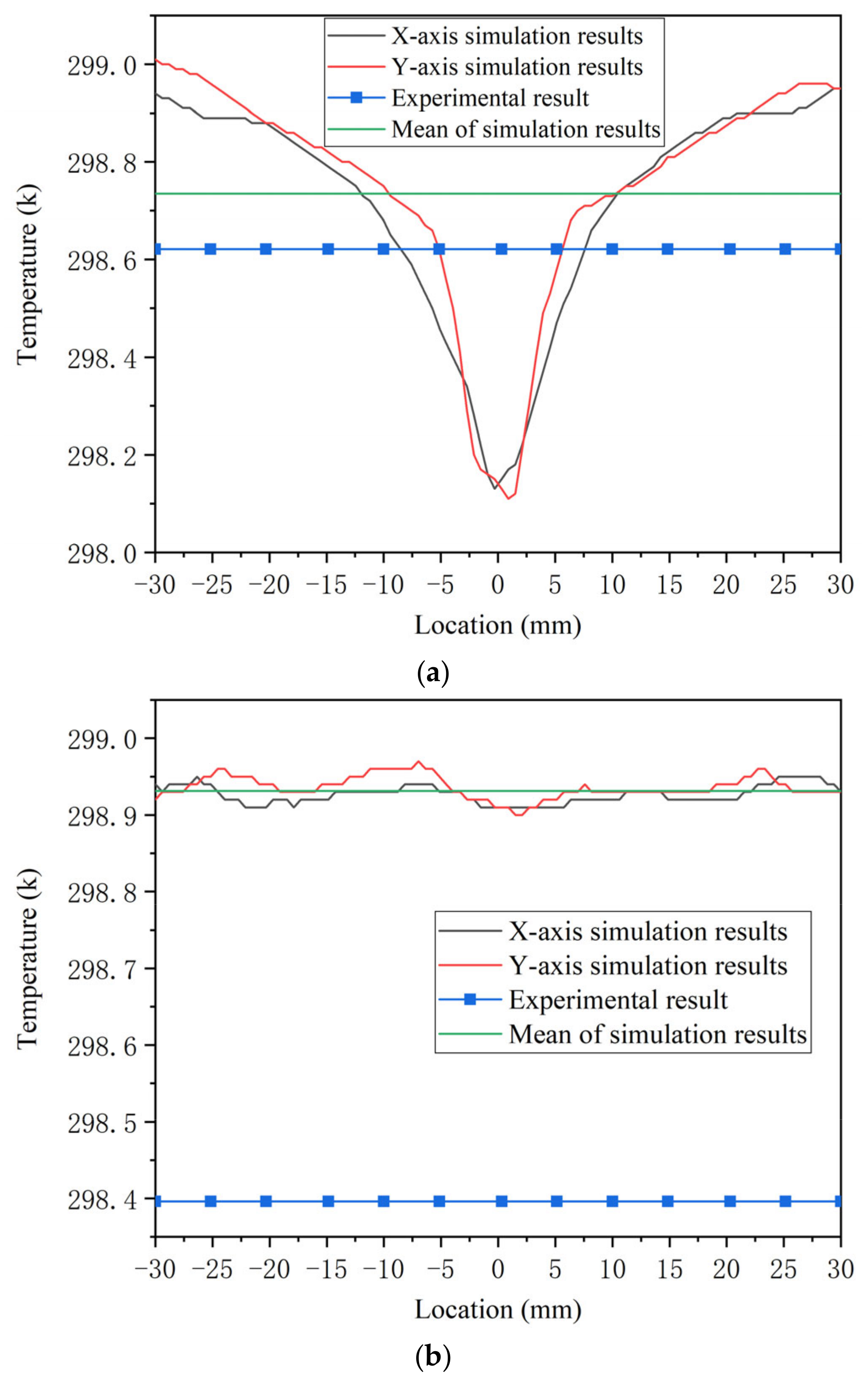
2.2. Experimental Data for Model Validation

This study is based on the previous research results on the heating efficiency of different types of susceptors in the induction heating process 4. In the case of determining the fluid inlet temperature of the heating device, the accuracy of the model was verified by comparing the outlet temperature. The experimental device involved in the research process is shown in Figure 4. Previous studies were carried out at a flow rate of 2 kg/min with a quartz tube with an inner diameter of 60 mm. The experimental process was repeated three times. The frequency excitation during the operation of the induction heating device, the inlet and outlet temperature of the fluid, and other parameters were taken as the mean of three trials. As shown in Figure 4, the static mixer-type susceptors were crossed in pairs into a group, and the susceptors with different geometric structures were distinguished by different crossing angles. Here, the 10° crossing angle (78 metal plates) and 15° crossing angle (52 metal plates) were selected. The experimental conditions and results from prior research are summarized in

Table 2. Experimental conditions and results from previous research.

Geometry	Frequency (kHz)	Current Drive (A)	Fluid Inlet Temperature (k)	Fluid Outlet Temperature (k)
10° (78 metal plates)	32.64	213	284.84	298.62
15° (52 metal plates)	31.23	215	284.69	298.40

. In addition, as mentioned previously, the coil material was copper, and the susceptor material was 304 stainless steel.

The experimental data in Table 2 were obtained from previous studies. Based on this, the simulation of low heating power was carried out, and the simulation results were compared with the experimental results to verify the accuracy of the model.

2.3. Simulation Settings

2.3.1. Different Cross Angle and Heating Power Comparison Simulation Settings

First, according to the experimental data recorded in Section 2.2, the susceptors with two different cross angles at low heating power were simulated and analyzed. The purpose was to compare the similarity between the simulation results and the experimental results and verify the accuracy of the simulation model. The actual power obtained by the susceptor was then increased by increasing the current excitation intensity at the coil interface, and the susceptor temperature distributions at two different crossing angles and heating powers were compared. The model establishment and the selection of boundary conditions in this stage are as follows.

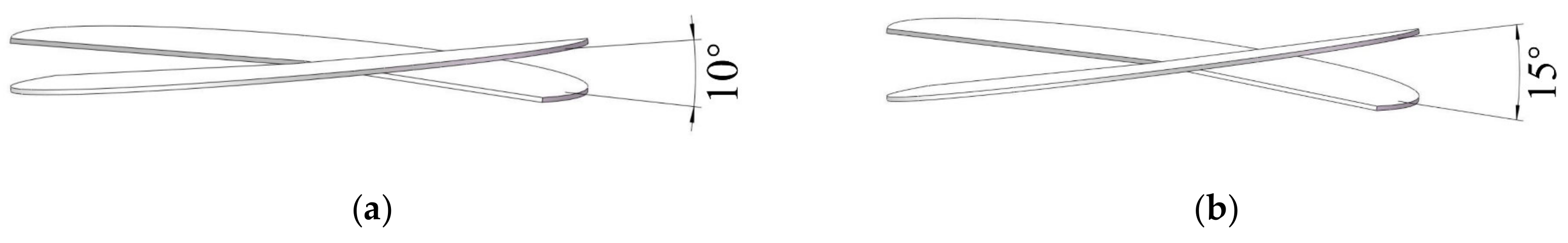
Two Cross Angles Involved in Simulation Process

First, based on the experiment, two kinds of susceptors with cross angles of 10° (78 metal plates) and 15° (52 metal plates) were simulated and analyzed. The model is shown in Figure 5.

In addition, in the high-power simulation stage, the intersecting metal plates in the susceptor were defined as a group. Considering the accuracy of the simulation and the feasibility of the calculation, the spacing between each group was limited to 0.24 mm as shown in Figure 6. At this time, the total heights of the susceptors with a 10° cross angle and a 15° cross angle were 230.75 mm and 220.76 mm, respectively. Because there was some difference in height, the total energy obtained with each of the two susceptors was later compared to avoid the impact of height difference on the results. The influence of susceptor spacing on the heating process will be discussed in the subsequent simulation section.

Boundary Condition

Boundary Condition Selection of Electromagnetic Field. After determining the geometric structure, the boundary conditions of electromagnetic simulation were determined. According to the research of previous scholars [27], the default boundary conditions were selected in the electromagnetic simulation. Parameters such as frequency and current excitation at low power were obtained in the experiment, and the current excitation at high power was set to 400 A, as shown in

Table 3. Simulation Boundary Condition Parameters of Low Heating Power Group.

Structure	Parameter
	Frequency (kHz)	Current (A)	Liquid Flow Rate (m/s)	Inlet Temperature (K)
10° (78 metal plates)	32.64	213	0.011789	284.75
15° (52 metal plates)	31.23	215	0.011789	284.75

and

Table 4. Simulation Boundary Condition Parameters of High Heating Power Group.

Structure	Parameter
	Frequency (kHz)	Current (A)	Liquid Flow Rate (m/s)	Inlet Temperature (K)
10°	32.64	400	0.011789	284.75
15°	31.23	400	0.011789	284.75

.

Boundary Condition Selection of Temperature Field. Then, the boundary conditions of fluid–solid heat transfer were determined. The average inlet temperatures of the fluid in the 10° and 15° groups during the previous experiment were 284.84 K and 284.69 K, respectively. In order to simplify the simulation process, the boundary conditions of the simulated fluid inlet temperature were taken between the above two values; thus, the error was less than 1 K and can be ignored. The subsequent simulation also used the fluid inlet temperature as the boundary condition. As mentioned earlier, in order to simplify the model, the outer wall, air heat transfer, and radiation heat transfer factors were ignored. Therefore, the lateral boundary conditions of the fluid domain were set to be adiabatic, and coupled heat transfer was applied between the susceptor and the fluid.

Boundary Condition Selection of Flow Field. In terms of flow parameters, the simulation analysis was carried out under a flow rate of 2 kg/min in the experimental stage. The inlet diameter was 60 mm, and the water density was 1 × 10³ kg/m³. The fluid velocity was obtained as a boundary condition with Equations (8) and (9)

$${\mathrm{q}}_{\mathrm{m}}{=\mathsf{\rho }\mathrm{q}}_{\mathrm{v}}$$

(8)

$${\mathrm{q}}_{\mathrm{v}}=\mathrm{uA}$$

(9)

where ${\mathrm{q}}_{\mathrm{m}}$ is the mass flow rate of fluid (kg/s); ρ is fluid density (kg/m³); ${\mathrm{q}}_{\mathrm{v}}$ is the fluid volume flow (m³/s); u is the fluid velocity (m/s); A is the circulation area (m²). In the calculation process, the fluid density ρ was approximately 1 × 10³ kg/m³, and the fluid velocity was approximately 0.011789 m/s using the experimental conditions.

The Reynolds number in the simulation can be calculated with Equation (10)

$${\mathrm{R}}_{\mathrm{e}}=\frac{\mathrm{ud}}{\mathrm{v}}$$

(10)

where u is the fluid velocity (m/s); because the pipe used in the experiment is a circular section, the proposed d is the pipe diameter (m); v is the kinematic viscosity of the water (m²/s). The dynamic viscosity of the water was $1.01\times {10}^{-3}$ pa·s. The Reynolds number at the fluid inlet was about 700, which is much lower than the lower critical Reynolds number. Therefore, the flow state of the fluid in the simulation process was laminar flow. The inlet of the fluid domain was set as the velocity inlet. The outlet setting refers to the method adopted by Cheng [28] in the numerical simulation of the finned fin–tube heat exchanger, which was set as outflow.

Finally, all of the boundary conditions are summarized in Table 3 and Table 4.

2.3.2. Susceptor Optimization Simulation Settings

First, the optimization of the susceptor was carried out for the geometric structure and physical parameters, and it did not involve the change of boundary conditions. The parameter settings in the simulation process are shown in

Table 5. Parameter settings of static mixer-type susceptor optimization simulation.

Simulation Parameter Setting
15° Cross Angle				10° Cross Angle
Changing outer angle parameters		Change material electric conductivity (S/m)		Changing the susceptor spacing (mm)			Change outer angle and chamfer
105°	120°	3.6 × 105	5.76 × 106	0.097	0.24	0.32	100°	110°

, and the parameters not mentioned in the table remain unchanged from those described in Table 4. The influence of geometric structure and physical parameters on temperature distribution was studied, and the static mixer-type susceptor was optimized.

First, the geometry optimization simulation of the 15° cross angle susceptor was carried out. The change of the outer angle of the susceptor will be described in detail in the form of pictures in Section 3.2.1. Then, the electric conductivity of the metal material was changed to study the influence of different material properties on the uniformity of temperature distribution.

Then, the optimization simulation was carried out for the 10° cross angle susceptor. First, the influence of the spacing between two groups of susceptors on the uniformity of temperature distribution was studied, and the related values are shown in Table 5. The outer angle of the 10° cross angle susceptor was optimized according to the simulation results of the 15° cross angle susceptor. The distance from the tip of the inner corner to the center of the outer arc was appropriately reduced during the simulation optimization of the 10° angle susceptor to ensure that the area of the through-hole did not change significantly before and after optimization. On this basis, the sharp corners were chamfered to further slow down the sharp corner effect. The geometric structure optimization of the 10° cross angle susceptor will be described in detail in the form of pictures in Section 3.3.2.

Finally, the magneto-thermal two-way coupling simulation was carried out for the susceptor structure with the best heating uniformity. First, the influence of thermal conductivity as it changed with temperature on the uniformity of temperature distribution was considered independent of the influence of thermal conductivity and electrical conductivity as they changed with temperature on temperature distribution.

3. Results and Discussion

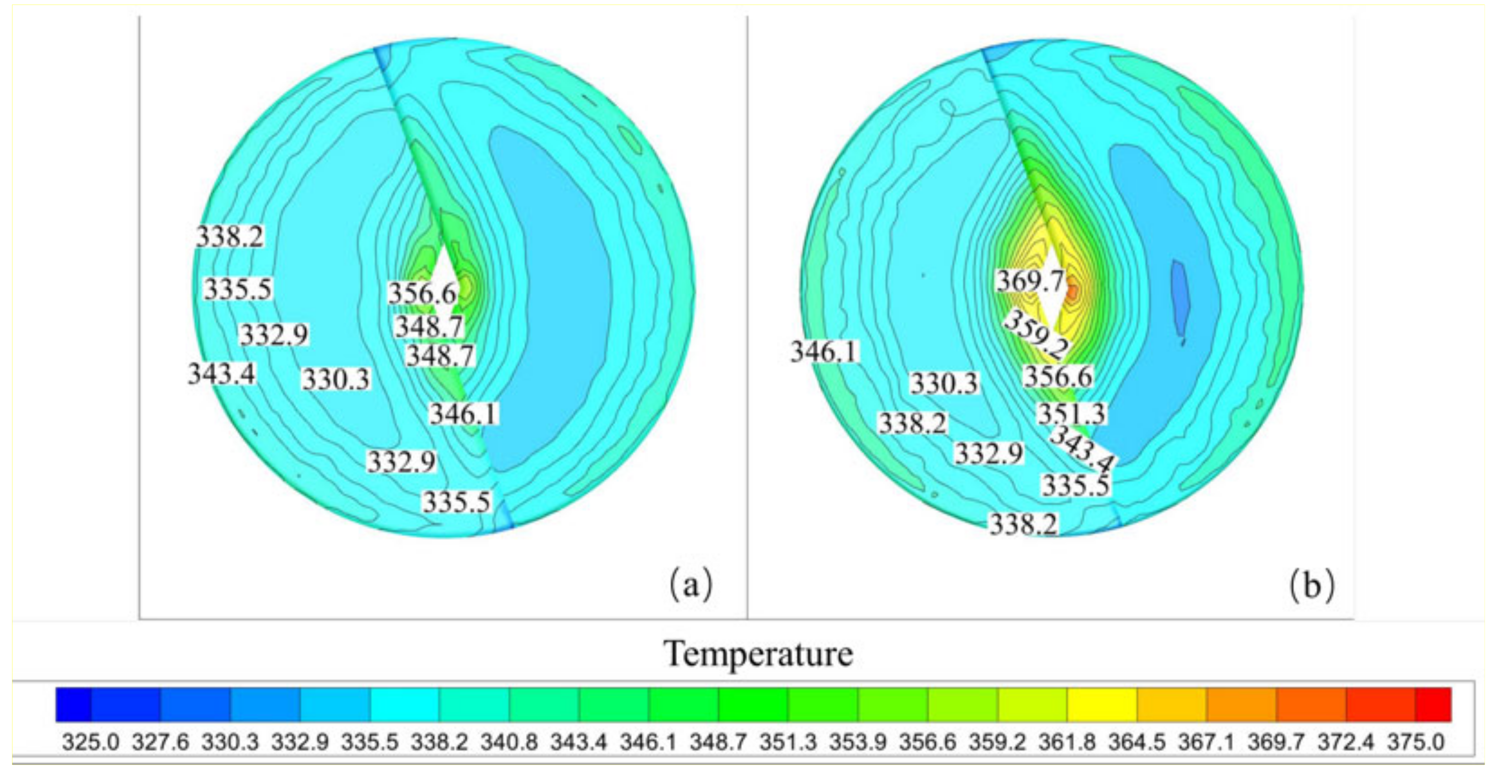
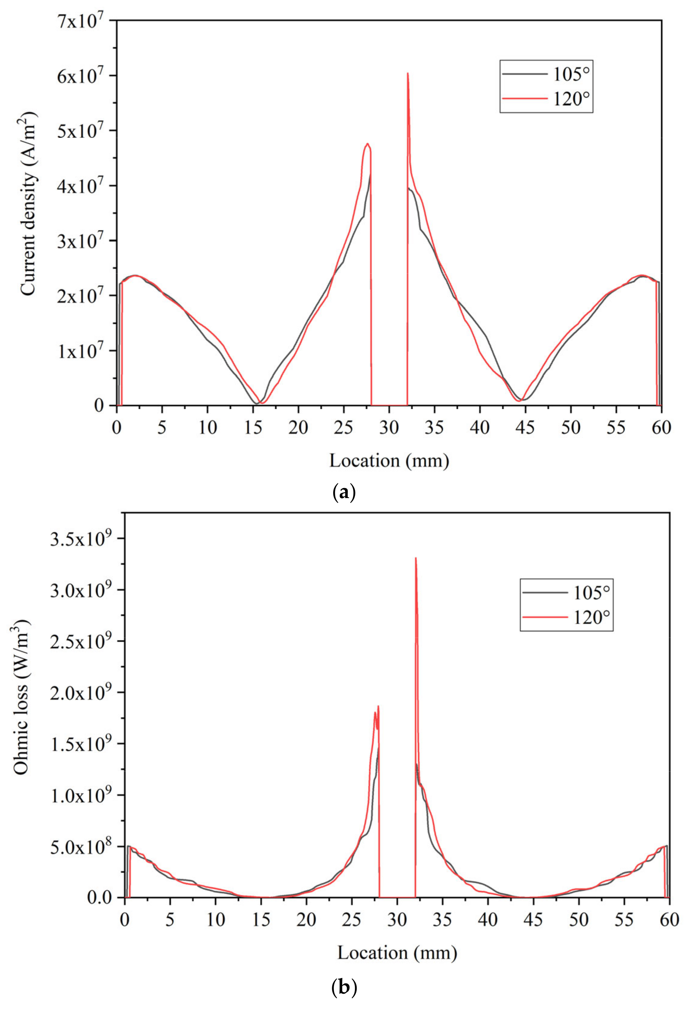
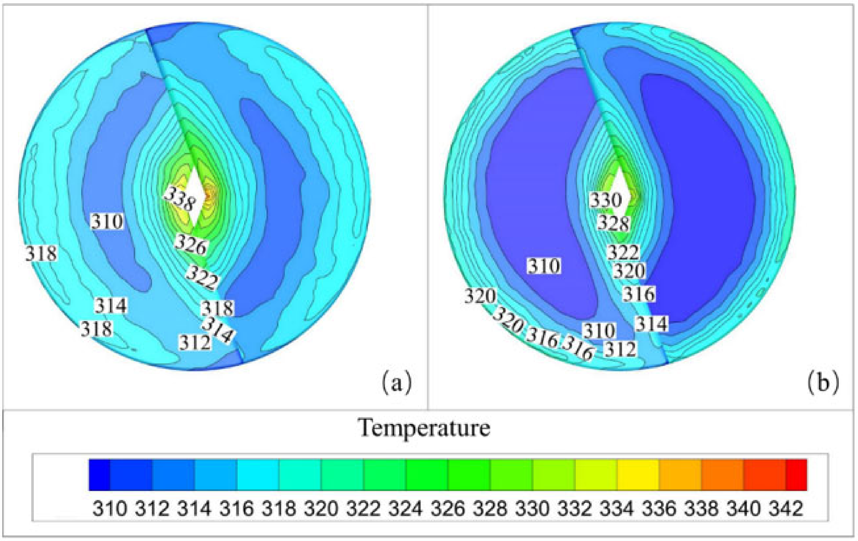
3.1. Effects of Different Crossing Angles and Power on Temperature Distribution

The temperature distribution of the outlet was obtained by simulating two different angle susceptors under low input power. The simulation results were compared with the experimental data recorded in Section 2.2 to verify the accuracy of the simulation model. The susceptor closest to the fluid inlet was defined as the first group of susceptors, and the center point of the first group of susceptors intersecting each other is the origin of the coordinate axis. At a distance of 0.23 m from the origin, the lines were drawn along the X-axis and the Y−axis, and the temperature changes were read. The mean values of all points at all positions of the comprehensive simulation results were compared with the experimental values. The comparison results are shown in Figure 7.

From the comparison between the mean value of the simulation results and the mean value of the experimental results, it can be seen that the accuracy of the simulation results is good, and the error between the simulation results and the experimental results is less than 1 K. Therefore, the accuracy of the simulation model is acceptable.

From the results of the low power simulation group, it is not difficult to see that the heating process of the susceptor was very uniform at low power, and the temperature difference between different positions of the susceptor outlet was within 1 K. However, first of all, the lower outlet temperature cannot be used for actual production, and second, it cannot clearly characterize the influence of different structures and materials on the uniformity of temperature distribution.

Considering the above two problems, the power obtained by the susceptor was improved by increasing the current excitation. The cross section of the susceptor with 10° cross angle was analyzed at the position of 0.15696 m and 0.17472 m from the origin, and the cross section of the susceptor with 15° cross angle was analyzed at the position of 0.15725 m and 0.17425 m from the origin. The temperature distribution of the two susceptors during heating at high power is shown in Figure 8.

The four positions described previously are the spacing regions between the two sets of susceptors. In Figure 8, it can be clearly seen that there was significant heat concentration at the junction of the two groups of susceptors located at the upper and lower poles of the cross section. However, in addition, the regular conclusions about the influence of two cross-angle susceptors on temperature uniformity cannot be summarized with this diagram. Therefore, the temperature distribution on the metal plate of 10° cross angle and 15° cross angle susceptor with the height of 0.17768 m and the height of 0.1785 m was studied, as shown in Figure 9.

It can be seen in Figure 9 that the temperature distribution on the metal plate of the susceptor with a 10° cross angle was more uniform than that of the susceptor with a 15° cross angle. This phenomenon can be explained as follows: under the same heating power, the energy distribution of the 10° cross angle susceptor was more dispersed due to the larger number of metal plates.

In fact, in the high–power simulation, the energy obtained with the 10° cross angle susceptor was about 63 w higher than that of the 15° crossing angle susceptor, though the difference can be ignored. However, because the susceptor with a 10° cross angle had 26 metal plates more than the susceptor with a 15° cross angle, the energy distribution was more dispersed, which ultimately leads to a more uniform temperature distribution during the heating process. In summary, between the 10° cross angle susceptor and the 15° cross angle susceptor, there was no significant difference in metal plate temperature distribution at the junction of the two groups, but from the metal plate surface temperature distribution can be judged 10° cross angle susceptor heating effect is better than 15° cross angle susceptor. However, even if the heating effect of the susceptor with a 10° cross angle was more uniform, heat concentration also occurred at the inner corners of the center of each group of susceptors. The cause of this phenomenon can be explained as the energy concentration caused by the corner effect, which was caused by the special geometric structure of the inner angle position. Therefore, the next optimization direction was to reduce the corner effect by changing the geometric structure.

3.2. Effect of Different Simulation Parameters on Heating Uniformity at 15° Cross Angle

3.2.1. Effect of Geometric Structure on Temperature Distribution Uniformity

As mentioned, the corner effect led to an energy concentration area at the inner corner of the susceptor, resulting in uneven temperature distribution. Therefore, optimization was performed from the perspective of changing the geometry of the susceptor to mitigate the corner effect. The structural change of the susceptor is shown in Figure 10, and the surface temperature distribution of the susceptor metal plate is shown in Figure 11.

Figure 11 shows the influence of two different geometric structures on the corner effect. It can be seen from the diagram that the intensity of the corner effect was proportional to the angle of the outer corner. The height of the two sets of metal plates recorded in Figure 11 was 0.1785 m; thus, a reference line was made along the X−axis at a height of 0.1785 m in the electromagnetic analysis software, enabling it to pass through the metal plate and output the current density and ohmic loss on the reference line, as shown in Figure 12.

It can be seen from Figure 12 that there was a significant current density and ohmic loss concentration at the sharp corner position when the outer corner was larger, which led to the temperature concentration at the sharp corner position described in Figure 11. In addition, the temperature distribution in the coupled heat transfer process of fluid and solid must also have been the result of the combined action of fluid flow and solid heat distribution. Separate analysis of the temperature distribution on the metal plate was one-sided. Therefore, the cross section was made at a height of 0.1785 m, and the velocity distributions in the X, Y, and Z directions were analyzed. The results are shown in Figure 13.

It can be seen from Figure 13 that when the outer angle was 105°, the fluid velocity at the outer edge and the center of the susceptor was significantly larger than it was when the outer angle was 120°. This allowed the susceptor structure with an external angle of 105° to generate more intense heat transfer, especially at the central through-hole. Under the combined action of the energy concentration caused by the corner effect and the low heat transfer coefficient caused by low flow rate, the temperature distribution of the 120° outer angle susceptor was not as uniform as that of the 105° outer angle susceptor.

3.2.2. Effect of Different Material Properties on Temperature Distribution

Referring to the method used by Bio et al. 18 in the study of induction heating thermochemical reactors in 2021, the effects of different electric conductivity rates on temperature distribution during induction heating were analyzed. The original conductivity was reduced four times to 3.6 × 10⁵ S/m and expanded four times to 5.76 × 10⁶ S/m. The simulation also defined the metal plate with a height of 0.1785 m for analysis. The results are shown in Figure 14.

First, it can be seen from the cloud distribution that the uniformity of heat distribution was inversely proportional to electric conductivity. This is consistent with the law of skin effect, which states that electric conductivity and skin depth are inversely proportional. The higher the electric conductivity, the more concentrated the heat distribution. Therefore, it is not difficult to draw the conclusion that for any susceptor structure used for fluid heating, the lower the electric conductivity of the material, the better the heating effect if it is evaluated only from the perspective of the influence of skin depth on heating uniformity.

However, it is worth noting that the actual power levels obtained by the susceptor with a conductivity of 3.6 × 10⁵ S/m and the susceptor with a conductivity of 5.76 × 10⁶ S/m were reduced by about $3\times {10}^3$ w compared with the conductivity of 1.44 × 10⁶ S/m when parameters such as the heating frequency current excitation intensity were constant. That is, the heating efficiency of both susceptors decreased. This phenomenon can be explained by the relationship between current intensity and workpiece resistance and the relationship between workpiece resistance and heat. First, using the same method as above, the change in the X−axis current density at an output height of 0.1785 m is shown in Figure 15.

It is not difficult to see from the line chart that there is a huge gap between the current density changes of the X−axis at 0.1785 m height under the two conductivity rates. This phenomenon can be explained as follows. As the voltage is constant, the current intensity is inversely proportional to resistance strength, but the workpiece heat Q is proportional to the current value. The influence of both current intensity and resistance intensity finally causes this phenomenon. This is also why Acero et al. [29] mentioned in their 2020 study that the metal layer should be kept at an appropriate thickness to maximize the equivalent resistance of each material.

3.3. Effect of Different Simulation Parameters on Heating Uniformity at 10° Cross Angle

3.3.1. Effect of Different Susceptor Spacing on Heating Uniformity

As mentioned above, there was spacing between each group of static mixer-type susceptors in the simulation process that did not exist in the actual experiment process. In order to study the error caused by this spacing in the simulation results, three levels of 0.097 mm, 0.24 mm, and 0.32 mm were selected for research. The results are shown in Figure 16.

It can be seen from Figure 16 that the temperature distribution at the spacing position did not show regular changes under different group spacing conditions, and the temperature values at similar positions under different spacing conditions did not show much difference. Therefore, it can be judged that the existence of the spacing did not affect the simulation results.

3.3.2. Effects of Different Geometric Structures on Temperature Distribution

The susceptor was optimized using the following three points. First, as mentioned earlier, the greater the number of metal plates, the more dispersed the energy, resulting in a more uniform temperature distribution on each metal plate. Secondly, the smaller the outer angle of the metal plate, the lower the influence of the corner effect on temperature distribution. Third, because the corner effect is characterized by a higher current intensity at the cusp position than at the smooth position, chamfering was performed at the position in Figure 17c to eliminate the cusp, as shown in Figure 17d, in order to further attenuate the cusp effect. In summary, the geometric structure of the susceptor with a 10° cross angle was optimized. The change of the geometric structure of the susceptor is shown in Figure 17, and the optimization result is shown in Figure 18.

It can be seen from the temperature distribution cloud map that the temperature amplitude of the sharp corner position was significantly reduced by combining the addition of the enlarged susceptor with the chamfering of the sharp corner position, and thus, the area occupied by the high temperature zone was expanded to a certain extent. Combining the above two points, it can be judged that the optimized susceptor obtained a more uniform temperature distribution.

As mentioned, the thermal conductivity and electrical conductivity of metal structures change with temperature during actual heating. Therefore, this study first analyzed the influence of thermal conductivity on tempera-ture distribution and then analyzed the influence of thermal conductivity and electri-cal conductivity on temperature distribution, as shown in Figure 19 and Figure 20, respectively.

It can be seen from the temperature distribution of Figure 19 that the change of thermal conductivity with temperature did not have a significant effect on the temperature distribution of the magneto-thermal coupling process. This appearance can be explained by the fact that the thermal conductivity changed too little with temperature in the experimental range; thus, it could not have had a significant effect on heat distribution.

Compared with Figure 19, the two simulation results shown in Figure 20 have obvious changes. Considering the change of electrical conductivity with temperature, the area of the high temperature zone was obviously larger than when not considering the change of electrical conductivity with temperature. This phenomenon can be explained as follows: the electrical conductivity of 304 stainless steel decreases with an increase in temperature, and the skin depth of metal under an alternating magnetic field is inversely proportional to electrical conductivity. Finally, the skin effect in the high temperature region of the susceptor was alleviated to a certain extent during the heating process. At the same time, the reference line was drawn using the same method as the previous comparison of current density, and the temperature change in the X−axis direction at a height of 0.162 m was obtained, as shown in Figure 21.

This value reflects the temperature change process inside the metal plate of the susceptor, which can best reflect the small change of temperature. It can be seen from the above diagram that the X−axis temperature obtained in the case of magneto-thermal two-way coupling was slightly higher than that of the case of single coupling with constant electrical conductivity. This trend is consistent with the phenomenon that induction heating efficiency increases with the change of workpiece resistance in a certain range. That is, the simulation considering the change of thermal conductivity and electric conductivity with temperature best reflects the temperature distribution in the actual heating process.

The final output was the temperature distribution of the fluid heated by the optimized 10° cross angle susceptor at a height of 0.25 m away from the last set of susceptors at 0.022 m. The temperature distribution at this position was analyzed as the temperature distribution at the heater outlet position, and the results are shown in Figure 22. It can be seen from Figure 22 that the temperature of the heated fluid through the susceptor increased by about 50K, and the average temperature at the outlet reached about 334 K when the inlet temperature was about 284.75K. The temperature difference between different positions of the outlet section was less than 1K, and the temperature distribution’s uniformity was good. The temperature distribution shown in the diagram can be explained by the fact that the flow velocity at the central through-hole was higher than it was around the through-hole during the heating process using the susceptor.

4. Conclusions

In this study, the heating process of static mixer-type susceptor was simulated. The susceptor was simulated and optimized in three aspects: different power comparisons, the influence of structural change on temperature distribution uniformity, and the influence of the physical property changes of metal material on temperature distribution uniformity. The simulation results are highly consistent with the experimental results.

First, the cross angle of the susceptor negatively correlated with heating uniformity. The smaller the crossing angle, the more metal plates the susceptor contains, the more dispersed the energy and the more uniform the temperature distribution. The simulation results show that the maximum temperature of the 10° cross angle susceptor was about 13 K lower than that of the 15° cross angle susceptor at the energy concentration point.

Second, the geometric structure of the susceptor metal plate had a significant impact on the uniformity of temperature distribution. Reducing the outer angle of the susceptor slowed down the corner effect while increasing the flow rate of the fluid at the center hole position and ultimately obtaining a more uniform temperature distribution. Under the combined influence of flow rate change and corner effect change, the maximum temperature of the energy concentration point was reduced by about 11 K.

Furthermore, higher electric conductivity led to aggravation of the skin effect, which led to uneven temperature distribution. In the actual heating process, the electric conductivity of metal materials decreased with increasing temperature. The decrease of conductivity in a certain range was beneficial to the conversion of energy from electromagnetic energy to thermal energy and also to the uniform distribution of energy.

Finally, the spacing between each group of susceptors did not have a significant impact on the uniformity of temperature distribution. When the optimized susceptor was used to heat the flowing liquid, the temperature difference between different positions at the outlet was less than 1K, and temperature distribution uniformity was better.

The application prospect of this study is that the optimized static mixer-type susceptor can be used to heat flowing low-viscosity liquid food materials more evenly to achieve the purpose of thermal sterilization of liquid food; thus, it can reduce the problem of local material quality degradation caused by uneven temperature distribution during thermal effect sterilization.

References

1. Lucia, O.; Maussion, P.; Dede, E.J.; Burdio, J.M. Induction Heating Technology and Its Applications: Past Developments, Current Technology, and Future Challenges. IEEE Trans. Ind. Electron. 2014, 61, 2509–2520. [Google Scholar] [CrossRef]
2. Başaran, A.; Yilmaz, T.; Çivi, C. Energy and exergy analysis of induction-assisted batch processing in food production: A case study—Strawberry jam production. J. Therm. Anal. Calorim. 2020, 140, 1871–1882. [Google Scholar] [CrossRef]
3. Başaran, A.; Yılmaz, T.; Azgın, Ş.T.; Çivi, C. Comparison of drinking milk production with conventional and novel inductive heating in pasteurization in terms of energetic, exergetic, economic and environmental aspects. J. Clean. Prod. 2021, 317, 128280. [Google Scholar] [CrossRef]
4. Shi, M.; Fu, J.; Xu, Q.; Wu, L.; Wang, R.; Zheng, Z.; Li, Z. Non-contact heating efficiency of flowing liquid effected by different susceptors in high-frequency induction heating system. Int. J. Chem. React. Eng. 2022. [Google Scholar] [CrossRef]
5. Başaran, A.; Yılmaz, T.; Çivi, C. Application of inductive forced heating as a new approach to food industry heat exchangers: A case study Tomato paste. J. Therm. Anal. Calorim. 2018, 134, 2265–2274. [Google Scholar] [CrossRef]
6. Kittiamornkul, N.; Yingcharoen, S.; Khumsap, T.; Inklab, L. A small pasteurization system using magnetic induction for coconut juice. In Proceedings of the 2017 14th International Conference on Electrical Engineering/Electronics, Computer, Telecommunications and Information Technology (ECTI-CON), Phuket, Thailand, 27–30 June 2017; pp. 381–384. [Google Scholar] [CrossRef]
7. Unver, U. Efficiency analysis of induction air heater and investigation of distribution of energy losses. Teh. Vjesn.-Tech. Gaz. 2016, 23, 1259–1267. [Google Scholar] [CrossRef]
8. Wang, G.; Wan, Z.; Yang, X. Induction heating by magnetic microbeads for pasteurization of liquid whole eggs. J. Food Eng. 2020, 284, 110079. [Google Scholar] [CrossRef]
9. Idakiev, V.V.; Lazarova, P.V.; Bück, A.; Tsotsas, E.; Mörl, L. Inductive heating of fluidized beds: Drying of particulate solids. Powder Technol. 2017, 306, 26–33. [Google Scholar] [CrossRef]
10. Idakiev, V.V.; Steinke, C.; Sondej, F.; Bück, A.; Tsotsas, E.; Mörl, L. Inductive heating of fluidized beds: Spray coating process. Powder Technol. 2018, 328, 26–37. [Google Scholar] [CrossRef]
11. Kilic, V.T.; Unal, C.; Demir, H.V. High-efficiency flow-through induction heating. IET Power Electron. 2020, 13, 2119–2126. [Google Scholar] [CrossRef]
12. Icier, F.; Kaya, O. Mathematical modeling of continuous induction heating of sour cherry juice. J. Food Process Eng. 2022, 45, e14180. [Google Scholar] [CrossRef]
13. Kawakami, H.; Llave, Y.; Fukuoka, M.; Sakai, N. CFD analysis of the convection flow in the pan during induction heating and gas range heating. J. Food Eng. 2013, 116, 726–736. [Google Scholar] [CrossRef]
14. Kastillo, P.J.; Martínez, J.; Jonathan, R.; Villacís, S.P.; Orozco, M. Computational fluid dynamic analysis of olive oil in different induction pots. In Proceedings of the 1st Pan-American Congress on Computational Mechanics—PANACM2015, Buenos-Aires, Argentina, 27–29 April 2015. [Google Scholar]
15. Eom, H.; Park, K. Fully-Coupled Numerical Analysis of High-Frequency Induction Heating for Thin-Wall Injection Molding. Polym.-Plast. Technol. Eng. 2009, 48, 1070–1077. [Google Scholar] [CrossRef]
16. Chang, S.J.; Xie, P.C.; He, X.T.; Yang, W.M. Numerical Simulation of Temperature Field in Barrel of Injection Molding Machine during Induction Heating Process Based on ANSYS Software. Adv. Mater. Res. 2009, 87–88, 16–21. [Google Scholar] [CrossRef]
17. Kranjc, M.; Zupanic, A.; Miklavcic, D.; Jarm, T. Numerical analysis and thermographic investigation of induction heating. Int. J. Heat Mass Transf. 2010, 53, 3585–3591. [Google Scholar] [CrossRef]
18. Jang, J.; Chiu, Y. Numerical and experimental thermal analysis for a metallic hollow cylinder subjected to step-wise electro-magnetic induction heating. Appl. Therm. Eng. 2007, 27, 1883–1894. [Google Scholar] [CrossRef]
19. Bio Gassi, K.; Guene Lougou, B.; Baysal, M.; Ahouannou, C. Thermal and electrical performance analysis of induction heating based-thermochemical reactor for heat storage integration into power systems. Int. J. Energy Res. 2021, 45, 17982–18001. [Google Scholar] [CrossRef]
20. Tian, S.; Barigou, M. Assessing the potential of using chaotic advection flow for thermal food processing in heating tubes. J. Food Eng. 2016, 177, 9–20. [Google Scholar] [CrossRef]
21. Fang, Z.; Gong, Z.; Li, Y.; Yao, Y. Simulation and Experiment of Electromagnetic Induction Heating System Based on ANSYS. Exp. Technol. Manag. 2021, 38, 129–133. [Google Scholar] [CrossRef]
22. Zhu, G.; Wu, L.; Xie, D.; Tong, Z.; Wang, G.; Chen, H.; Chen, Z.; Ren, G. Effect of Plastic Deformation and Fatigue Damage on Electromagnetic Properties of 304 Austenitic Stainless Steel. Chin. J. Appl. Mech. 2017, 34, 842–847. [Google Scholar] [CrossRef]
23. Cao, B.; Iwamoto, T.; Bhattacharjee, P.P. An experimental study on strain-induced martensitic transformation behavior in SUS304 austenitic stainless steel during higher strain rate deformation by continuous evaluation of relative magnetic permeability. Mater. Sci. Eng. A 2020, 774, 138927. [Google Scholar] [CrossRef]
24. Wang, Y.; Liu, Z.; Xie, L.; Ma, Y.; Gao, C. Temperature Control Method of Thin Film Electric Heater Based on PTC Characteristics. Autom. Instrum. 2021, 36, 37–40. [Google Scholar] [CrossRef]
25. Qiu, H.; Huo, Y. Influence of physical parameters on simulation of welding temperature field. J. Shandong Jianzhu Univ. 2015, 30, 452–455. [Google Scholar]
26. Zhu, Y. Research and Application of Magneto-Thermo-Structural Coupling Numerical Simulation on Induction Heating. Doctoral Dissertation, Shanghai Jiao Tong University, Shanghai, China, 2019. [Google Scholar] [CrossRef]
27. Li, Q. The Design Ofthe Ih Electric Cooker’s Thermalfieldand Magnetic Field; University of Electronic Science and Technology of China: Chengdu, China, 2014. [Google Scholar]
28. Cheng, X. Numerical Simulation of Fin-Tube Heat Exchanger and Multi-Objective Optimization Design of Structural Parameters; East China University of Technology: Nanchang, China, 2021. [Google Scholar] [CrossRef]
29. Acero, J.; Lope, I.; Carretero, C.; Burdio, J.M. Adapting of Non-Metallic Cookware for Induction Heating Technology via Thin-Layer Non-Magnetic Conductive Coatings. IEEE Access 2020, 8, 11219–11227. [Google Scholar] [CrossRef]
Figure 1. Modeling of susceptor, coil, and fluid domain in simulation process. (a) Two groups of static mixer-type susceptors with 10° inclination angle (39 groups in total). (b) Simplified static mixer-type susceptor structure. (c) Geometric model for magnetic field analysis. (d) Geometric model for flow field analysis.
Processes 11 00533 g001
Figure 2. Simulation process of (a) one-way coupling and (b) two-way coupling.
Processes 11 00533 g002
Figure 3. Model grids for electromagnetic analysis with (a) 10° cross angle and (b) 15° cross angle meshes.
Processes 11 00533 g003
Figure 4. Experimental device diagram of heating flowing liquid by loading static mixer-type susceptor.
Processes 11 00533 g004
Figure 5. Static mixer-type susceptors with different cross angles: (a) 10° cross angle and (b) 15° cross angle.
Processes 11 00533 g005
Figure 6. Two groups of susceptor interval diagram (susceptor front view).
Processes 11 00533 g006
Figure 7. Comparison of axial temperature changes and mean values at the outlet position of the susceptor at cross angles of (a) 10° and (b) 15°.
Processes 11 00533 g007
Figure 8. Temperature distribution at different positions: (a) 10° cross angle at 0.15696 m; (b) 10° cross angle at 0.17472 m; (c) 15° cross angle at 0.15725 m; (d) 15° cross angle at 0.17425 m.
Processes 11 00533 g008
Figure 9. Temperature distribution on the metal plates of the susceptors at different angles: (a) 10° cross angle susceptor; (b) 15° cross angle susceptor.
Processes 11 00533 g009
Figure 10. 15° cross angle susceptor with two different geometries (susceptor top view): (a) outer angle 105° and (b) outer angle 120°.
Processes 11 00533 g010
Figure 11. Temperature distribution of 15° cross angle susceptor with two different geometric structures: (a) outer angle 105° and (b) outer angle 120°.
Processes 11 00533 g011
Figure 12. Current density and ohmic loss on the X−axis square line reference line: (a) current density change and (b) ohmic loss change.
Processes 11 00533 g012
Figure 13. Fluid velocity components in three directions: (a) 105° outer angle, X−axis velocity component; (b) 120° outer angle, X−axis velocity component; (c) 105° outer angle, Y−axis velocity component; (d) 120° outer angle, Y−axis velocity component; (e) 105° outer angle, Z−axis velocity component; (f) 120° outer angle, Z−axis velocity component.
Processes 11 00533 g013
Figure 14. Temperature distribution under different electric conductivity rates: (a) 3.6 × 10⁵ S/m and (b) 5.76 × 10⁶ S/m.
Processes 11 00533 g014
Figure 15. Current density variation under two conductivity rates.
Processes 11 00533 g015
Figure 16. Effect of different spacings on temperature distribution: (a) 0.097 mm; (b) 0.24 mm; (c) 0.32 mm.
Processes 11 00533 g016
Figure 17. Comparison of the geometric structure of the susceptor before and after chamfering: (a) susceptor with chamfering; (b) susceptor without chamfering; (c) local amplification of position I to indicate the distance between the chamfered radian and the original inner corner tip position to the center of the outer arc; (d) local amplification of position II to indicate the distance from the inner corner tip position to the center of the outer arc.
Processes 11 00533 g017
Figure 18. 10° cross angle susceptor optimization results: (a) chamfer-optimized; (b) not chamfer-optimized.
Processes 11 00533 g018
Figure 19. Simulation results considering temperature dependence of metal thermal conductivity: (a) thermal conductivity changing in response to temperature; (b) thermal conductivity not changing in response to temperature.
Processes 11 00533 g019
Figure 20. Simulation results considering temperature dependence of metal electrical conductivity: (a) electrical conductivity changing in response to temperature; (b) electrical conductivity not changing in response to temperature.
Processes 11 00533 g020
Figure 21. Comparison of temperature changes on metal plates under unidirectional and bidirectional magneto−thermal coupling.
Processes 11 00533 g021
Figure 22. Temperature distribution at 0.25 m height.
Processes 11 00533 g022