Abstract
The data distribution of the vibration signal under different speed conditions of the gearbox is different, which leads to reduced accuracy of fault diagnosis. In this regard, this paper proposes a deep transfer fault diagnosis algorithm combining adaptive multi-threshold segmentation and subdomain adaptation. First of all, in the data acquisition stage, a non-contact, easy-to-arrange, and low-cost sound pressure sensor is used to collect equipment signals, which effectively solves the problems of contact installation limitations and increasingly strict layout requirements faced by traditional vibration signal-based methods. The continuous wavelet transform (CWT) is then used to convert the original vibration signal of the device into time–frequency image samples. Further, to highlight the target fault characteristics of the samples, the gray wolf optimization algorithm (GWO) is combined with symmetric cross entropy (SCE) to perform adaptive multi-threshold segmentation on the image samples. A convolutional neural network (CNN) is then used to extract the common features of the source domain samples and the target domain samples. Additionally, the local maximum mean discrepancy (LMMD) is introduced into the parameter space of the deep fully connected layer of the network to align the sub-field edge distribution of deep features so as to reduce the distribution difference of sub-class fault features under different working conditions and improve the diagnostic accuracy of the model. Finally, to verify the effectiveness of the proposed diagnosis method, a fault preset experiment of the gearbox under variable speed conditions is carried out. The results show that compared to other diagnostic methods, the method in this paper has higher diagnostic accuracy and superiority.
1. Introduction
Due to the rapid development of industrial intelligence, data monitoring and deep intelligence algorithms are widely used in equipment health monitoring, especially in fault diagnosis [1,2,3]. The process of fault diagnosis mainly includes data acquisition, data preprocessing, feature extraction, and classifier diagnosis. At present, in terms of data acquisition, most of the fault diagnosis models use the vibration signal of the equipment as the original training sample. Mariela Cerrada et al. [4] realized gearbox fault diagnosis by extracting the time and frequency features from the vibration signal of the spur gearbox and combining them with the genetic algorithm and the random forest classifier. Wen et al. [5] designed a novel convolutional network, which took the vibration datasets of motor bearings, self-priming centrifugal pumps, and axial piston hydraulic pumps as the original input and then used the deep learning ability of the network to achieve fault diagnosis of different equipment. Hou et al. [6] proposed a novel feature selection method that can eliminate redundant and invalid interference information in the vibration signal of the bearing and ensure the best feature subset with low computational complexity. Although the vibration signal can directly reflect vibration excitation during operation of the equipment, in the process of data acquisition there are disadvantages, such as high requirements for the placement of the vibration sensor, the ease with which it may fall off, and high installation cost. As a non-destructive testing technology, the acoustic signal method can collect data without affecting the installation of the sensor and has the advantages of low consumption cost and easy layout while acquiring equipment fault signals. Adam Glowacz [7] analyzed the fault acoustic signal of a single-phase asynchronous motor and developed and implemented a method of acoustic signal feature extraction, with the fault diagnosis of the motor bearing finally realized through the KNN classifier. Yao et al. [8] proposed a novel fault diagnosis algorithm for planetary gearboxes based on acoustic signals, and the proposed comprehensive characteristic parameters can significantly improve the accuracy of fault diagnosis compared to single characteristic parameters. Wail M. Adaileh [9] proposed an experimental study on the detection of engine faults using acoustic signals through analysis of the domain parameters, such as RMS amplitude, peak amplitude, and energy for condition monitoring, and fault diagnosis of internal combustion engines.
In terms of data preprocessing and feature extraction, because of the rapid development of deep networks in recent years, their powerful deep self-learning capabilities have been widely used. More and more studies use raw 1D fault signals or simple 2D time–frequency transformed images as training samples. Gao et al. [10] used the continuous wavelet transform (CWT) of complex Morlet wavelets to obtain the time–frequency characteristics of the vibration signal through joint time–frequency analysis and obtained the input of the deep network through normalization. Wang et al. [11] used short-time Fourier transform (STFT) to transform the raw vibration signal of the device to obtain the corresponding time–frequency map. The features of the time–frequency map are then adaptively extracted using a convolutional neural network (CNN). Gu et al. [12] proposed a hybrid fault diagnosis method for rolling bearings based on CWT and CNN, which is suitable for small sample diagnosis. Zhang et al. [13] used STFT transform theory to obtain input images, introduced a scaled exponential linear unit (SELU) function in the network to avoid excessive ‘dead’ nodes during training, and used hierarchical regularization to obtain better training results. Although the diagnosis method of time–frequency images combined with a deep network has obtained good diagnosis results, the single signal time–frequency conversion cannot effectively highlight the fault characteristics of the sample. In this regard, some scholars have introduced the theory of threshold segmentation in image preprocessing, trying to highlight the edge factors of different key components in image samples. Threshold segmentation is a method of processing an image into a high-contrast, easy-to-recognize image with a suitable pixel value as a boundary. Therefore, it can effectively distinguish the target interest boundary in time–frequency image samples. Rakoth Kandan Sambandam et al. [14] combined the dragonfly optimization algorithm and the threshold segmentation algorithm to obtain the global optimal solution of segmentation by effectively exploring the solution space. Shan et al. [15] segmented massive infrared images based on chroma-saturated luminance space to distinguish defective device images and extracted defective device regions from the images. Finally, the improved residual network is trained for fault feature learning through an online mining method. Manikanta Prahlad Manda et al. [16] effectively calculated the threshold for image segmentation based on the concept of one-dimensional histogram approximation, and finally verified the excellent performance of the method on various infrared images. The above research results show that the threshold segmentation algorithm can effectively improve the boundaries of different components in image samples, thereby improving the accuracy of classification.
In the classification stage of fault diagnosis, in recent years, fault diagnosis algorithms based on deep learning have shown they can adaptively learn and mine the deep-level features of data and achieve better diagnosis results than traditional feature engineering [17,18]. However, most of the deep learning diagnosis algorithms currently assume that the training data and the test data have the same probability distribution, which is often untenable in the actual industrial environment where the operating environment is changeable and the working conditions are complex. For example, changes in operating conditions, such as equipment speed, load, normal aging, and deepening damage to faulty parts, will lead to real-time changes in the distribution of data. At this point, when a new data stream is entered, the diagnostic accuracy of the model trained on the historical data will decrease. In recent years, the concept of transfer learning has been put forward to solve the above-mentioned limitations in the fault diagnosis of industrial equipment and has been widely used. The basic problem is how to solve new fields (target domain). Obviously, a certain similarity between the source domain and the target domain is a major premise of transfer learning. Therefore, the main work of transfer learning is to reduce the feature difference between the data in the source domain and the target domain and improve the transferability between the data so as to achieve the purpose of knowledge transfer and reduce the amount of data participation in the target domain [19,20,21]. In addition, transfer learning takes full advantage of deep learning in expressing high-dimensional abstract features of data. Deep learning methods represented by deep networks map two sets of data with similar but different distributions into a high-dimensional shared feature space and use transfer methods to minimize inter-domain differences when the edge distribution of the data becomes clearer [22]. Among them, domain adaptation, as one of the subdomains of transfer learning, mainly solves the problem of knowledge transfer between two domains with the same feature space and label space (isomorphic domain) through distance measurement. The metrics for distance measurement include maximum mean difference (MMD), KL divergence, and Wasserstein distance, among others. Yang et al. [23] used conditional domain adversarial (CDA) domain adaptive networks and joint maximum mean deviation standard (JMMD) to align the source and target domains, effectively realizing cross-domain diagnosis under different operating conditions. Xiao et al. [24] used convolutional neural networks to extract multi-level features of the device’s original vibration signal. Further, the maximum mean difference (MMD) can be added during the training of the network to impose constraints on the parameters of the CNN, thereby reducing the distribution differences in the characteristics of the source and target domain data. Zhu et al. [25] used the Kuhn–Munkres algorithm to improve the calculation process of the Wasserstein distance, which can better learn transferable features between labeled and un-labeled signals from different forms of devices. Finally, the effectiveness of the proposed method is verified under different mechanical parts and transmission scenarios. The above research shows that transfer methods, such as domain adaptation based on the distance metric method, can effectively reduce the feature difference between the source domain and the target domain and realize the knowledge transfer between the same or similar types of devices, which solves the above-mentioned key constraint of constant data distribution in practical industrial environments. However, in practice, the data in different domains not only have significant differences in marginal distributions, but also in conditional distributions. By aligning the marginal distribution of data in different domains, the invariant eigenvectors of the domain can be learned. However, if the differences in conditional distribution between different domain data are not taken into account, the optimal cross-domain classification hyperplane will be difficult to obtain. In response, Wang et al. [26] built a subdomain adaptive transfer learning network by stacking two convolutional building blocks to extract transferable features from raw data. Pseudo-label learning is then modified and the target subdomain of each class is constructed, which reduces the marginal and conditional distribution deviations and improves the classification performance and generalization of the network. Tian et al. [27] used a multi-branch network structure to respectively match the feature space distribution of each source domain and target domain in order to align the subdomain distributions in the same category of different domains and diagnose the device status. Wang et al. [28] proposed a joint subdomain adaptive network (JSAN) that reduces the difference between two domains by jointly local maximum mean disparity, improving the diagnostic accuracy. The above study shows that the conditional distribution difference between subdomains is also an important factor to be considered in domain adaptive diagnosis.
Inspired by the above research, we propose a gearbox acoustic signal fault diagnosis algorithm based on adaptive multi-threshold segmentation and subdomain adaptation to solve the problem of cross-domain adaptive fault diagnosis under the condition of variable gearbox speed. The main innovations in this article are as follows:
(1) Signal monitoring using acoustic sensors makes it easier to collect fault signals from gearbox equipment without contact.
(2) The combination of a gray wolf optimization algorithm (GWO) and symmetric cross entropy (SCE) can realize the adaptive multi-threshold segmentation of CWT time–frequency map samples of the gearbox, thereby enhancing the boundary of target fault characteristics.
(3) We design a subdomain adaptive network model based on a CNN structure and add the local maximum mean discrepancy (LMMD) metric criterion to the fully connected layer parameter space in the deep network. At the same time, the differences in the data distribution of sub-categories within the domain are considered before the difference is eliminated.
Finally, we verify the effectiveness and superiority of the method with the dataset from the gearbox variable speed experiment. The rest of the paper is organized as follows: Section 2 introduces the relevant theories in detail. Section 3 discusses the proposed fault diagnosis model and diagnosis process. Section 4 provides the process of preparing gearbox fault data, and the results of the fault diagnosis experiment are analyzed and discussed. Finally, the conclusions of this paper are elaborated in Section 5.
2. Methodology
2.1. Transfer Learning
Transfer learning is a new type of deep learning whose goal is to extract similar components (transfer components) between different but related domains so as to transfer knowledge from one domain to another. Among them, the original data domain and the target interest domain are called the source domain and the target domain, respectively [29,30]. To facilitate the description, the concepts of domain and task are first introduced. A domain consists of two parts, a d-dimensional feature space and a marginal probability distribution P(X), where X is a set of n samples, and each sample corresponds to a feature vector in the space , that is . Therefore, a domain can be represented by . Further introduce the concept of tasks, a task consists of a label space and a class prediction function . When given a feature vector, the class prediction function can predict its corresponding class label . From the probabilistic point of view, the label category can be denoted as , so the task can be denoted as . After the source domain and learning task , target domain and learning task are determined separately, or , that is, the distribution of the source domain and the target domain is different, transfer learning will use the tasks and knowledge of the source domain to help improve the computational performance of the target prediction function for the target domain data (see Figure 1) [31,32].
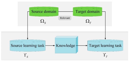
Figure 1.
Schematic diagram of transfer learning.
2.2. Subdomain Adaptation
Usually, in the transfer learning fault diagnosis of mechanical equipment, the data of the source domain and the target domain can be the data of the same equipment under different working conditions, or the data of the same model of different equipment. The tasks to be solved in both domains are the same, that is, both domains have the same fault category and classification tasks. Such transfer tasks are called domain adaptation and they are an important branch of transfer learning (see Figure 2) [33]. This paper intends to implement migration diagnosis under different rotational speed conditions on the same rotating mechanical equipment, that is, the feature space dimension and fault label space of the source domain and target domain data are the same. Most of the current diagnosis algorithms only consider the alignment of the global marginal distribution between the source domain and the target domain. However, the lack of distinguishing the conditional distributions between the same subclass of faults will lead to a decrease in the accuracy of transfer fault diagnosis (as shown in Figure 3a). On this basis, the concept of subdomain adaptation is further proposed, that is, when the global distribution of the source domain data and the target domain data is roughly the same, the conditional distribution between the subdomain fault data is further aligned [34]. This will reduce the distribution difference of sub-type fault data under different working conditions of the equipment, thereby improving the accuracy of fault diagnosis (as shown in Figure 3b).
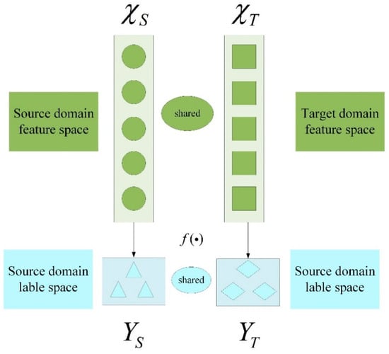
Figure 2.
Domain Adaptive Schematic.
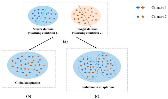
Figure 3.
Subdomain adaptation schematic: (a) source and target domain conditions; (b) global adaptation; (c) subdomain adaptation.
2.3. Continuous Wavelet Transform (CWT)
CWT has good localized analysis ability and multi-resolution analysis ability for equipment fault signals and has the characteristic of window adaptation compared to time–frequency conversion methods such as STFT. It uses a limited length wavelet base with an attenuation effect and locates the time node at which the signal frequency component appears via telescopic transformation and translation of the wavelet. For a series of time series, the wavelet function can move in the time dimension and compare the window signals at different positions one by one to obtain the wavelet coefficients. The larger the wavelet coefficients, the better the fitting degree of the wavelet and the signal. In the calculation, the convolution of the wavelet function and the window signal are used as the wavelet coefficient under the window. Therefore, the length of the window and the length of the wavelet are the same. In the frequency domain, the length and frequency of the wavelet are changed by stretching or compressing the length of the wavelet to realize the wavelet coefficients at different frequencies. Correspondingly, the window length also varies with the wavelet length. Combining the wavelet coefficients at different frequencies, the wavelet coefficient map of the time–frequency transform is obtained. The specific calculation process is as follows [35].
Assuming that both the input signal and the wavelet basis function satisfy , and represents a square-integrable real number space, the continuous wavelet transform of the input signal can be expressed as [36]:
In the formula, a and respectively represent the scale parameter and displacement parameter in the wavelet transformation. Further, the displacement and scale expansion of the wavelet base in the transformation process are represented by . represents the complex conjugate value of , and the symbol represents the inner product operation. The frequency domain form of wavelet transform can be expressed as,
In the formula, represents the Fourier transform of the signal ; represents the complex conjugate value of the Fourier transform of the wavelet basis function .
2.4. Adaptive Multi-Threshold Segmentation
2.4.1. Symmetric Cross Entropy (SCE)
Cross-entropy is used in Shannon information theory to measure the difference between two probability distributions. Suppose and are two distributions distributed on the probability space , then the cross-entropy of to is defined as [37]:
where refers to the correct distribution and refers to the approximate estimated distribution. Cross entropy is used to estimate the distance difference between distributions.
However, considering that it does not have distance symmetry, Brink et al. [38] developed the concept of symmetric cross entropy (SCE). SCE essentially adds the forward Kullback divergence and the backward Kullback divergence, which makes the cross entropy symmetrical and thus allows it to become a real distance measure. The expression of symmetric cross entropy is:
On this basis, image adaptive multi-threshold segmentation is carried out with SCE as the standard. Even if Formula (5) takes the minimum value of x to be the optimal threshold,
Generalizing at most thresholds is performed to find a set of thresholds () that minimize the entropy value.
2.4.2. Gray Wolf Optimization Algorithm (GWO)
The gray wolf optimization algorithm (GWO) is a swarm intelligence optimization algorithm that was proposed by Mirjalili et al. from Griffith University in Australia in 2014 [39]. The algorithm is inspired by the hunting activities of gray wolves and has the characteristics of few parameters, strong convergence performance, and easy implementation. In recent years, the GWO algorithm has been widely and successfully applied in parameter optimization, image classification, and other fields. The algorithm divides the wolves into four levels (, , , and ) according to the hierarchy of the wolf society, as shown in Figure 4.
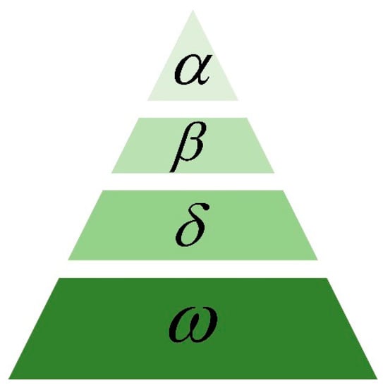
Figure 4.
Subdomain adaptation schematic.
The three gray wolves closest to the prey are named , and in order from near to far, corresponding to the optimal solution, the second optimal solution and the third optimal solution of the fitness function respectively; the remaining gray wolves are named uniformly as , corresponding to other candidate solutions. , and guide to search for prey, update location around , and . The entire hunting optimization process is shown in Figure 5, which mainly includes:
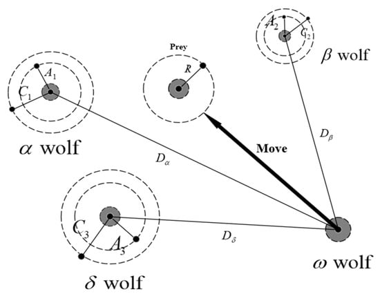
Figure 5.
The hunting optimization process diagram of gray wolves.
(1) Surrounding the prey. The behavior of surrounding the prey can be represented by the following computational procedure [40]:
In the formula, represents the distance between the prey and the gray wolf, and are the coefficient vectors, and represent the position vector of the prey and the gray wolf, respectively, and t is the current number of iterations.
(2) Attacking and searching for prey. Since the locations of the wolves in relation to the prey is unknown, the location update of during the hunting process is guided by , and . The behavior of attacking prey can be described as:
In the formula, , , represent the distances from to , and respectively, is a random number with a value of [0, 1], , , and represent the current location of , , and :
moves to , and according to the direction and step size specified in Formula (10), and Formula (5) represents the final position of . , and predict the location of the prey, randomly update the location around the prey. When the prey stops moving, the gray wolf completes the hunting behavior by attacking the prey.
2.4.3. Adaptive Multi-Threshold Segmentation Based on GWO-SCE
Due to the differences between different picture samples, especially in the time–frequency pictures with changing working conditions, it is more difficult to highlight the fault features. Therefore, the intelligent optimization algorithm can be used to optimize the threshold value to achieve the effect of adaptively obtaining the best threshold value. According to the SCE threshold segmentation principle in Section 2.4.1, to obtain the final threshold, it is necessary to find the corresponding minimum entropy value. Therefore, choose as the optimized fitness function:
H(x) represents the image cross entropy at different thresholds, and the optimization goal of the algorithm is to find an optimal set of thresholds so that the corresponding H(x) values are minimized. When the GWO algorithm iteration is over, it is considered that H(x) gets the smallest optimization value and that the fault feature boundary in the image has been effectively highlighted. When the threshold number changes from 1 to 4, the corresponding optimal fitness function values are constantly getting smaller: 1.0343 × 10⁶, 4.9 × 10⁵, 2.54 × 10⁵, 1.78 × 10⁵, respectively. When the threshold number is 4, the value of H(x) is the smallest and the segmentation effect is the best.
Further, to verify the effectiveness of the GWO-SCE adaptive multi-threshold segmentation method, we take the Lena image as an example (Figure 6a) and set the number of threshold segmentations to 1, 2, 3, and 4, respectively, with the optimization boundary set to [0, 255] (because the pixel value of the image ranges from 0 to 255). The number of wolves is set to 50, and the maximum number of iterations is set to 100. The experimental results are shown in Figure 6b–e.
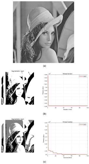
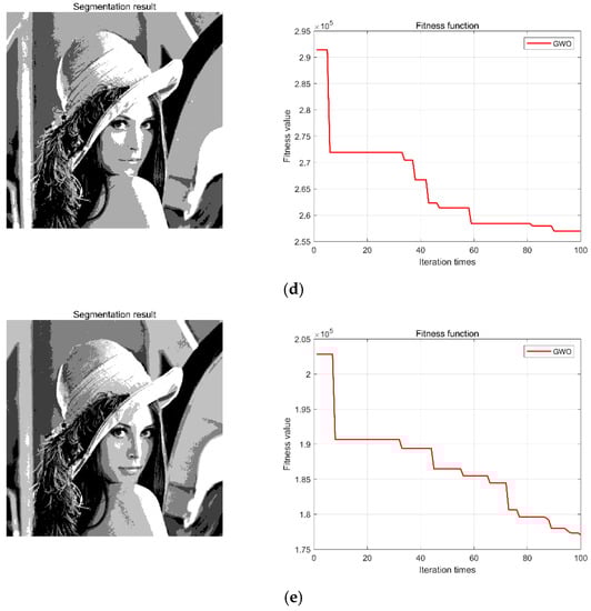
Figure 6.
Adaptive multi-threshold segmentation results of the Lena image. (a) Lena image; (b) single threshold segmentation and GWO iteration results; (c) two threshold segmentations and GWO iteration results; (d) three threshold segmentations and GWO iteration results; (e) four threshold segmentations and GWO iteration results.
It can be concluded from the experimental results in Figure 6 that the algorithm quickly achieved convergence and reached the minimum value of the fitness function at the 100th iteration, which indicates that the GWO-SCE algorithm has effective optimization ability. When the threshold number changes from 1 to 4, the corresponding optimal fitness function values are constantly getting smaller: 1.0343 × 10⁶, 4.9 × 10⁵, 2.54 × 10⁵, 1.78 × 10⁵, respectively. According to the entropy value theorem, the smaller the entropy value, the more information the image contains. Therefore, after optimization, the key information and features in the image are effectively highlighted and segmented, which is very useful for the learning and application of transferable features of image samples using deep networks.
2.5. Convolutional Neural Network (CNN)
The convolutional neural network is a unique neural network structure that was discovered when the neurons for local perception and direction selection were studied in the brains of cats. It is also a commonly used network in deep learning. It has strong feature learning ability, can effectively avoid the loss of local information, and performs well in the field of image classification. Its basic structure consists of an input layer, a convolutional layer, a pooling layer, a fully connected layer, and an output layer, as shown in Figure 7 [41,42].
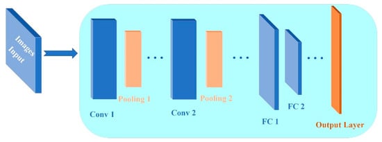
Figure 7.
Basic structure diagram of a CNN.
Among them, the calculation formula of the convolutional layer is:
where X represents the input image set, z represents the z-th output image, j represents the number of layers of the neural network, represents the input of the j-th layer, represents the output of the j-th layer, represents the convolution kernel, represents the bias, represents the activation function.
In the pooling layer, the max pooling function or the average pooling function is used for feature mapping, thereby reducing the dimension of the feature map and the amount of training calculations; however, this does not change the number of feature maps. The calculation formula of the pooling layer is:
where represents the k-th output image, represents the feature map with output size , represents the weight connection coefficient, represents the bias, and down (∙) represents the pooling function.
In a deep network, being fully connected means that neurons in each layer establish a weighted relationship with neurons in the previous layer.
The number of input images for the fully connected layer is l and the size is .
First, the input l image matrices are expanded in columns and then connected end to end according to the output order of the previous layer. Thus, it is spliced into , a one-dimensional feature column vector that is finally mapped to the corresponding category of the output layer. The mapping expression between the fully connected layer and the output layer is:
where represents the g-th value of the output layer, x represents the feature vector, represents the weight connection coefficient (weight value), represents the bias, and the activation function is generally the Softmax function. Finally, the output of the fully connected layer is divided into corresponding categories through the Softmax function [43,44].
2.6. Maximum Mean Difference (MMD)
The maximum difference in means is based on a nuclear two-sample test that rejects or accepts the null hypothesis for the observed sample, which is defined as a nonparametric distance measure in the reproducing kernel Hilbert space (RKHS) that measures the difference in the distributions of two datasets. In recent years, MMD has been widely used in the field of domain adaptation to perform cross-domain adaptation of features through minimization of the MMD distance between the source domain and target domain . The square of the MMD distance between the source dataset and target domain dataset is defined as [45,46]:
where H is the RKHS and and are Gaussian kernel functions.
In the formula, is the bandwidth of the kernel function, which can take multiple different values to calculate the MMD and superimpose its calculation results to form the so-called multi-core MMD.
3. CNN-Based Subdomain Adaptive Fault Diagnosis
Aiming at the inconsistency of characteristic distribution of fault state signal data collected under the different operating conditions of gearboxes, a subdomain adaptive depth transfer diagnosis method is proposed. The method mainly consists of two parts: transfer fault feature extraction and subdomain adaptation. Self-designed CNNs can be used to extract common features of samples; the subdomain adaptation uses the adaptive layer to learn the transfer knowledge, uses the local maximum mean discrepancy (LMMD) metric for conditional distribution difference calculation, and aligns the subdomains to achieve gearbox transfer learning for different operating conditions.
3.1. Subdomain Adaptive Deep Network Model
Based on quantitative research on feature transferability in deep convolutional networks, the general feature extraction layer mainly extracts the general features of the source domain data and the target domain data, and the difference between the two domains is mainly reflected in the fully connected layer (adaptive layer). Based on this theory, the subdomain adaptive network model proposed in this paper is shown in Figure 8. The number of layers and the network parameter settings are shown in Table 1.
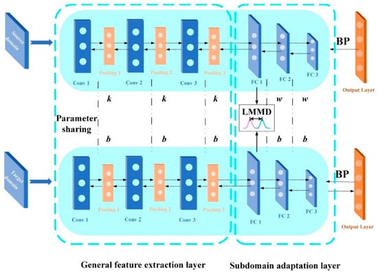
Figure 8.
Subdomain adaptive network model.

Table 1.
Subdomain adaptive network structure and parameter settings.
After the CWT time–frequency map samples of different speeds are put into the network, the convolutional layer extracts and learns the general features of the image. Further, the first layer of the fully connected network is set as the adaptive layer, and the LMMD metric is used for subdomain adaptation. Finally, a Softmax classifier performs fault diagnosis on the target domain’s work–case dataset. The objective function f optimized during training is:
In the formula, is the cross entropy loss function, is the subdomain adaptation function, and the total number of adaptive layers is denoted by L. In this paper, the LMMD metric is added to the first fully connected layer, thus L = 1. As a nonparametric distance estimation between two distributions, MMD is mainly used to measure the difference between the source domain distribution and the target domain distribution; for the subdomain adaptation problem, LMMD needs to be introduced:
In the formula, and are the weights of and belonging to the c-th class, respectively, which can be expressed as:
In the formula, is the c-th label of the input vector . Further, the ground-truth labels are used to calculate the weights of samples in the source domain. For the samples in the target domain, the deep neural network uses the learned probability distribution to represent the probability that the sample is recognized as a certain category. The weights of the target domain are therefore calculated using the predicted labels of the network. In implementing the adaptation process of deep network layers, the activation factor needs to be known. Given domains subject to probability distributions p and q, respectively, the network will generate activations for and in the adaptive layer. Therefore, the subdomain adaptation function is:
In the formula, is the activation factor of the l-th layer (). In the network training process, the objective function that needs to be finally optimized is:
3.2. Fault Diagnosis Algorithm Flow
The complete adaptive diagnosis algorithm flow from this paper is shown in Figure 9.
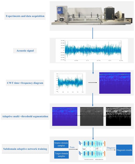
Figure 9.
Fault diagnosis strategy flowchart.
(1) Carry out the fault preset experiment and perform acoustic signal acquisition under the variable speed conditions of the gearbox while preprocessing the data to obtain digital samples.
(2) Perform CWT conversion on the signal to obtain two-dimensional time–frequency image samples.
(3) Adaptive multi-threshold segmentation is performed on the image samples to obtain the source domain sample and target domain sample required for the input of the network model.
(4) The source domain sample and target domain sample are entered into the subdomain adaptive network model for training and diagnosis, and the diagnosis results of the gear box target’s working condition data are obtained.
4. Case Study
4.1. Data Preparation
In this paper, the gear and bearing fault preset experiments are carried out with the help of a mechanical fault comprehensive simulation test bench. The experimental object is a secondary spur gearbox (as shown in Figure 10), and the collected acoustic signal data are used as the follow-up analysis object. The composition of the test bench includes power and control parts, a bearing fault simulation part, a gearbox fault simulation part, and a data acquisition part. This paper mainly conducts the pre-fault experiment on the gearbox part of the test bench. This part is mainly composed of a secondary reduction spur gear box (which can realize the preset faults of gears, bearings, and composite cases), magnetic powder brakes (providing loads), and magnetic powder brake controllers (controlling load changes).
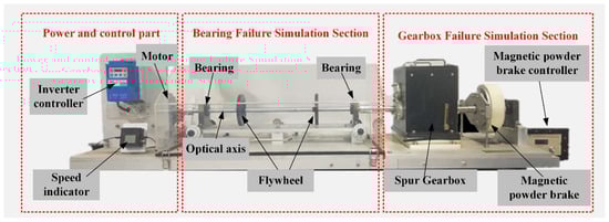
Figure 10.
Comprehensive fault simulation test bench.
The perspective view and internal structure diagram of the secondary reduction spur gear box are shown in Figure 11a,b. The number of teeth on the gears, from high-speed to low-speed shafts, are: 41, 79, 36, and 90, respectively. The preset faulty gear is gear 3, and the faulty bearing is located at the ER-16K bearing at the end cap in Figure 11b. The size parameters are shown in Table 2. Figure 11c shows the sound pressure sensor used in the experiment; the sensor is a YSV5001 high-precision ICP sound pressure sensor, which is mainly composed of an electret head and an ICP preamplifier, and its related performance indicators are shown in Table 3. These indicators meet the requirements of IEC61672 and GB/T3661 primary indicators. Figure 11d shows the process of acoustic signal acquisition, and the part marked in red in the figure is the sound pressure sensor.
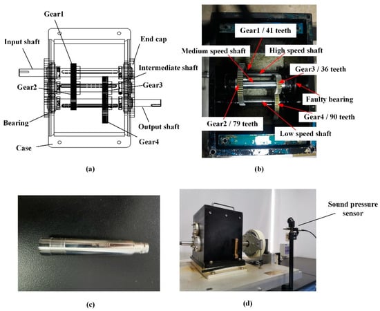
Figure 11.
(a) Perspective view of the gearbox; (b) internal structure of the gearbox; (c) sound pressure sensor; (d) view of signal acquisition.
Table 2.
Structural parameters of the ER-16K bearing.
Table 3.
Related technical indexes of the sound pressure sensor.
During the experiment, motor speed was controlled by the motor inverter controller or the MotorControl motor control software. MotorControl can change the motor speed by controlling the motor frequency conversion controller to realize the constant speed and continuous variable speed of the motor. The data acquisition system consists of a sound pressure sensor and VQ-USB4/LF data acquisition board. The board consists of the data acquisition board itself and VibraQuest Pro signal analysis software. VibraQuest Pro is a versatile data acquisition and condition detection system that records signal data in real-time from data acquisition boards. Figure 12 shows the signal acquisition system and software used in the experiment.
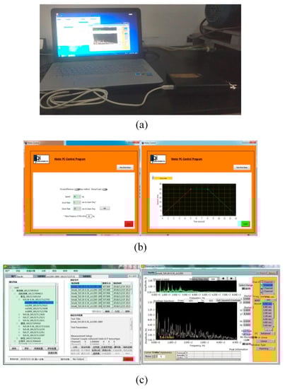
Figure 12.
(a) Data collection systems; (b) motor control software; (c) VibraQuest Pro software.
In the preset fault experiment in this paper, the fault types for gear settings include a missing tooth fault, broken tooth fault, and wear fault. The failure types for bearing settings include an inner ring failure, outer ring failure, and single ball failure. The fault is processed by pre-processing a deep groove with a width of 0.5 mm on the bearing outer ring, inner ring, and ball body. The relevant components corresponding to the six fault conditions are shown in Figure 13. Table 4 details the relevant information of the seven states of the gearbox under a single working condition.
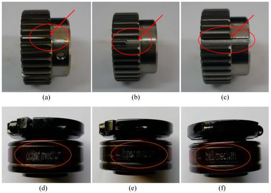
Figure 13.
(a) Missing gear; (b) broken gear; (c) uniform worn gear; (d) bearing outer fault; (e) bearing inner fault; (f) bearing rolling ball fault.
Table 4.
Gear and bearing fault status types.
In the experiment, the combined working conditions of different rotational speeds are set, and the acoustic signals of the normal state and the six fault states of the gearbox with different working conditions are collected respectively. In each experiment, the signal acquisition time was 48 s and the procedure was repeated 10 times. The design of the combined working conditions of different loads and speeds is shown in Table 4. A total of 5000 sampling points were used as a vibration sequence sample and 120 samples were taken for each set of fault data. Further, according to the working condition design in Table 5, we created six transfer learning tasks, namely , , , , , . The transfer task indicates that the data of working condition A are the source domain, and the data of working condition B are the target domain.
Table 5.
Design of the experimental conditions.
Further, we use CWT to convert the one-dimensional acoustic signal into a —dimensional RGB color time–frequency map with three channels (m and n are the length and width of the image, respectively, and three represents the number of primary color channels). To reduce the amount of computation, the RGB images are converted into —dimensional grayscale images. The adaptive multi-threshold segmentation method from Section 2.4 is used to perform adaptive threshold segmentation on the gray image samples. The specific processing process is shown in Figure 14. Due to limited article space, only the sample preparation process for the F5 fault signals under condition A (1200 rpm and 5 Nm) is listed here. The results of the experiments at different thresholds are shown in Figure 15.
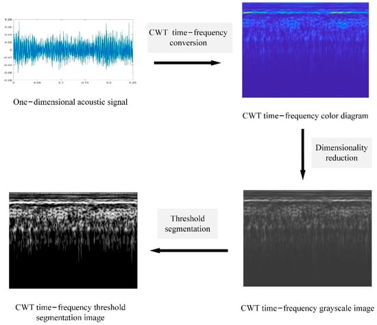
Figure 14.
Processing of image samples.
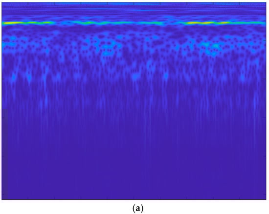
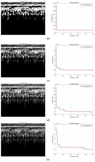
Figure 15.
Adaptive multi-threshold segmentation results of the F5 CWT image: (a) F5 CWT image; (b) single threshold segmentation and GWO iteration results; (c) two threshold segmentations and GWO iteration results; (d) three threshold segmentations and GWO iteration results; (e) four threshold segmentations and GWO iteration results.
From the experiment results in Figure 15, it can be seen that compared to the original CWT time–frequency map, the boundary of the image feature components after threshold segmentation is well highlighted, and with the increase in threshold number, the types and levels of components are also clearer. The corresponding fitness function values become smaller, with values of 7.907 × 10⁶, 4.49 × 10⁶, 2.75 × 10⁶, 1.88 × 10⁶, respectively. That is, when the threshold number is four, the cross entropy of the image reaches the minimum value and the fault classification feature information contained in the image is the greatest. In addition, after the threshold number exceeds five, the calculation amount and calculation time of sample processing become longer. Therefore, combined with the diagnostic effect and timeliness, the number of threshold segments is selected as four.
Further, the threshold segmentation results of the seven types of fault signal are shown in Figure 16. Due to limited article space, we have only listed the processing results of case A (1200 rpm and 5 Nm). Finally, 120 grayscale samples were obtained from the data of each fault type under the four speed conditions.
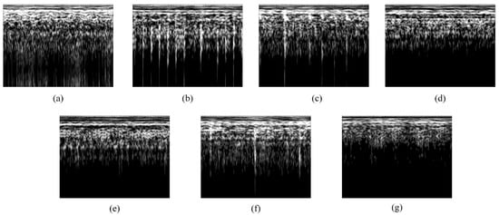
Figure 16.
Threshold segmentation processing results for different types of fault signals under case A: (a) F1 fault; (b) F2 fault; (c) F3 fault; (d) F4 fault; (e) F5 fault; (f) F6 fault; and (g) F7 fault.
4.2. Experimental Results
The source domain samples and target domain samples are entered into the subdomain adaptive network for training, and the parameter settings of the network during the training process are shown in Table 6. The average value of 10 fault diagnosis results is shown in Table 7. Figure 17 shows the network training and loss function curves for different transfer tasks.
Table 6.
Network hyperparameter settings.
Table 7.
Fault diagnosis results.
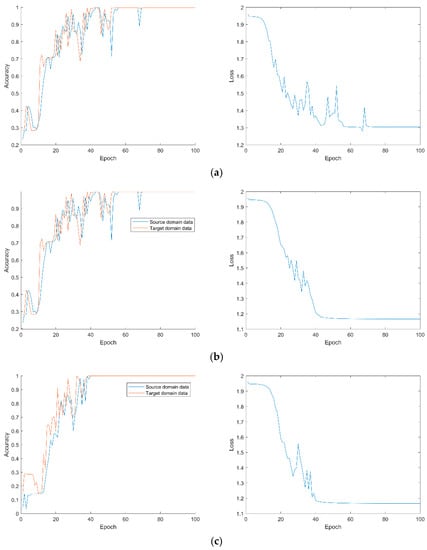
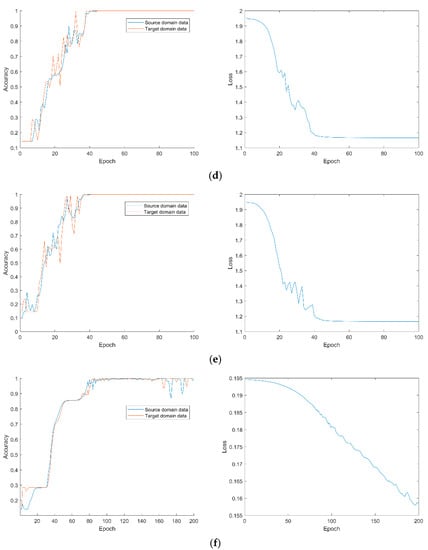
Figure 17.
Network training and loss function curves under different transfer tasks: (a)transfer task ; (b) transfer task ; (c) transfer task ; (d) transfer task ; (e) transfer task ; (f) transfer task .
From the above experimental results, in different transfer tasks, the proposed subdomain diagnosis fault algorithm can obtain high diagnosis accuracy, and the average diagnosis accuracy of the target domain reaches more than 99.84%. This shows that the characteristic knowledge between fault data under different rotational speed conditions has been transferred well, which proves the superiority of the algorithm in this paper. To further verify the fault features learned from the deep parameter space of the network, the effectiveness of cross-domain feature learning for subdomain adaptation was assessed. Using t-distributed stochastic neighbor embedding (t-SNE), the visualization is performed by mapping high-level feature representations from raw feature space to 2D space [47]. The visualized results are shown in Figure 18.
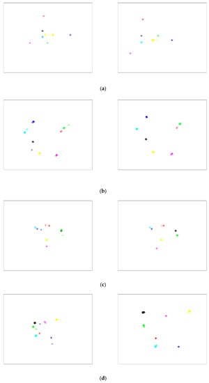
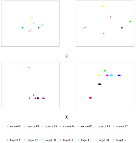
Figure 18.
Visualization of fully connected layer transfer features: (a) transfer task ; (b) transfer task ; (c) transfer task ; (d) transfer task ; (e) transfer task ; (f) transfer task .
The left column of Figure 18 illustrates that, without subdomain adaptive training, different types of data in the source domain are better classified but data obfuscation occurs in the target domain. The data distribution difference between the source domain and the target domain has not been effectively adapted to the domain, indicating that the knowledge of fault features is not transferred between domains. This resulted in a large number of diagnostic misjudgments. Observing the column on the right side of Figure 18 leads to the conclusion that, after the data is adaptively trained on subdomains, the fault features of the source and target domains are projected to the same region after deep learning and transfer. It can be observed that not only are the classification characteristics of the source domain data well distinguished, but the classification characteristics of the target domain are also consistent with the distribution of the source domain, a high-precision distinction. Therefore, the accuracy and effect of fault diagnosis have been greatly improved.
4.3. Small Sample Performance Analysis
To verify the diagnosis effect of the proposed fault diagnosis algorithm under the small sample diagnosis condition, the sample sizes for the source domain and target domain data in the transfer task were set to 40, 60, 80, 100, and 120, respectively. The average of ten experimental results is shown in Table 8 and Figure 19.
Table 8.
Diagnostic performance of the algorithm with different sample sizes.
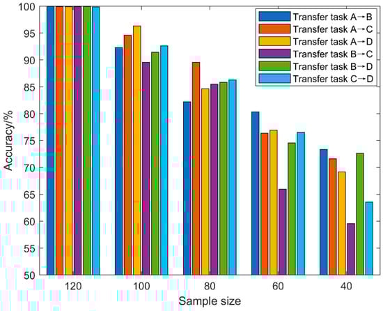
Figure 19.
Diagnostic performance graph of the algorithm under different sample sizes.
From the experimental results in Figure 19, it can be clearly concluded that the proposed fault diagnosis algorithm does not experience a large decline in diagnostic accuracy when the sample size drops sharply. On the contrary, because of the powerful feature learning ability of the deep network and the adaptive component training in the fully connected layer, the effective features in the sample can be learned and applied, and the failure accuracy rate can be maintained above 59%. At the same time, the fluctuation of diagnostic accuracy indicates that, in fault diagnosis based on deep networks, the accuracy of fault diagnosis can be improved by increasing the sample size.
4.4. Method Performance Comparison Analysis
To further verify the effectiveness of the diagnostic algorithm proposed in this paper, other diagnostic models are used for comparative analysis. Model 1 is the traditional machine learning classifier support vector machine (SVM, G1) [48]. Model 2 is the network model used in this paper but the samples are not segmented by a GWO-SCE adaptive multi-threshold, and only the CWT time–frequency transform (G2) is performed [49]. Model 3 replaces the domain distance measurement criterion with MMD (G3) [25]. Model 4 replaces the domain distance measurement criterion with the Wasserstein metric (G4) [50]. Model 5 is a domain adversarial neural network (DANN) that employs a domain discriminator to adversarially train the model to learn domain-invariant features (G5) across source and target domains. The method in this paper is denoted by G6. The average of ten experimental results is shown in Table 9 and Figure 20, where the training sample size was 120.
Table 9.
Diagnostic performance under different diagnostic methods.
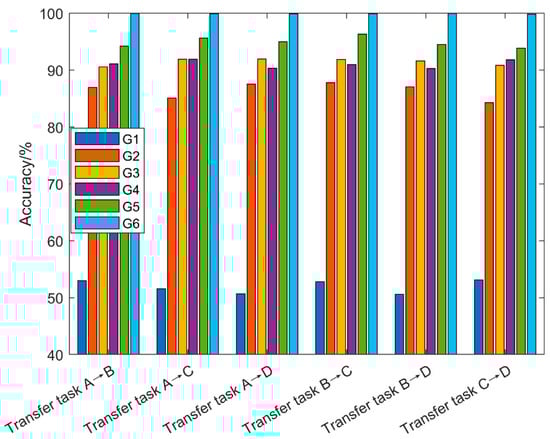
Figure 20.
Diagnostic performance graph under different diagnostic methods.
The following conclusions can be drawn from the above experimental results: (1) As a machine learning method, SVM cannot learn the deep-level features of image samples and cannot maintain high diagnostic accuracy when the data distribution of samples changes. (2) The CWT time–frequency map without threshold segmentation is used in the training process of the G2 model, and the diagnosis result is lower than that of the G6 model. This shows that GWO-SCE adaptive multi-threshold segmentation can better highlight the fault feature boundary of image samples, which can greatly improve the accuracy of fault diagnosis. (3) The MMD and Wasserstein metric criteria are used in the G3 and G4 models, respectively, and the conditional distribution between sub-type faults in the field is not considered, thus the diagnostic accuracy is lower than that of the G6 model. (4) The domain adversarial training of the G5 model also only considers the reduction of inter-domain differences, while ignoring the elimination of intra-domain differences. Therefore, the fault diagnosis effect of the G5 model is also weaker than that of the G6 model. In summary, the fault diagnosis algorithm proposed in this paper has outstanding effectiveness and superiority in the face of fault diagnosis problems under cross-domain variable working conditions.
5. Conclusions
The role of fault diagnosis theory in the health management of equipment is increasing. Aiming at the cross-domain fault diagnosis of gearboxes under variable speed conditions, this paper proposes a fault diagnosis algorithm for gearboxes based on GWO-SCE threshold segmentation and subdomain adaptation. Through experimental verification, the following conclusions are drawn.
(1) This paper uses the sound pressure sensor’s advantages of no contact, easy placement, and low cost to acoustically collect the fault signal of a gearbox, which effectively solves the problems of traditional vibration acceleration sensors, such as the limitation of contact-based installation and increasingly strict layout requirements.
(2) The adaptive multi-threshold segmentation method based on GWO-SCE can segment and highlight the effective fault components in CWT time–frequency images, which greatly helps the deep network learn the fault feature of the samples and then transfer them.
(3) The subdomain adaptive network adds the LMMD metric in the depth parameter space, which not only reduces the data distribution difference between the source and target domains, but also considers the conditional distribution between sub-class fault data. The experimental results of fault diagnosis show that the network model can complete the cross-domain transfer diagnosis under the condition of variable gearbox speed with high diagnostic accuracy.
As a fault diagnosis algorithm combining time–frequency analysis and a deep network, this research method can provide theoretical support and reference for equipment health management technology represented by fault diagnosis. In the future, seeking more effective time–frequency analysis technology, a greater number of targeted domain distance metrics, and network structures with stronger learning ability should be the direction of further research.
Author Contributions
Writing—original draft preparation, Y.L.; supervision, J.K.; data curation, L.W.; data curation, Y.B.; writing—review & editing, C.G.; writing—review & editing, project administration, W.Y. All authors have read and agreed to the published version of the manuscript.
Funding
This research was funded by [the Natural Science Foundation of China] grant number [No. 71871220].
Institutional Review Board Statement
Not applicable.
Informed Consent Statement
Not applicable.
Data Availability Statement
Not applicable.
Conflicts of Interest
The authors of this article declare that there are no known competing financial interest or personal relationships that could influence the work of this article.
References
- Chen, X.; Zhang, B.; Gao, D. Bearing fault diagnosis base on multi-scale CNN and LSTM model. J. Intell. Manuf. 2021, 32, 971–987. [Google Scholar] [CrossRef]
- Wang, X.; Mao, D.; Li, X. Bearing fault diagnosis based on vibro-acoustic data fusion and 1D-CNN network. Measurement 2021, 173, 108518. [Google Scholar] [CrossRef]
- Han, T.; Zhang, L.; Yin, Z.; Tan, A.C.C. Rolling bearing fault diagnosis with combined convolutional neural networks and support vector machine. Measurement 2021, 177, 109022. [Google Scholar] [CrossRef]
- Cerrada, M.; Zurita, G.; Cabrera, D.; Sánchez, R.-V.; Artés, M.; Li, C. Fault diagnosis in spur gears based on genetic algorithm and random forest. Mech. Syst. Signal Process. 2016, 70–71, 87–103. [Google Scholar] [CrossRef]
- Wen, L.; Li, X.; Gao, L.; Zhang, Y. A New Convolutional Neural Network-Based Data-Driven Fault Diagnosis Method. IEEE Trans. Ind. Electron. 2018, 65, 5990–5998. [Google Scholar] [CrossRef]
- Hui, K.H.; Ooi, C.S.; Lim, M.H.; Leong, M.S.; Al-Obaidi, S.M. An improved wrapper-based feature selection method for machinery fault diagnosis. PLoS ONE 2017, 12, e0189143. [Google Scholar] [CrossRef] [PubMed]
- Glowacz, A. Fault diagnosis of single-phase induction motor based on acoustic signals. Mech. Syst. Signal Process. 2019, 117, 65–80. [Google Scholar] [CrossRef]
- Yao, J.; Liu, C.; Song, K.; Feng, C.; Jiang, D. Fault diagnosis of planetary gearbox based on acoustic signals. Appl. Acoust. 2021, 181, 108151. [Google Scholar] [CrossRef]
- Adaileh, W.M. Engine fault diagnosis using acoustic signals. Appl. Mech. Mater. 2013, 295–298, 2013–2020. [Google Scholar] [CrossRef]
- Gao, D.; Zhu, Y.; Wang, X.; Yan, K.; Hong, J. A Fault Diagnosis Method of Rolling Bearing Based on Complex Morlet CWT and CNN. In Proceedings of the—2018 Prognostics and System Health Management Conference, PHM-Chongqing 2018, Chongqing, China, 26–28 October 2018; Institute of Electrical and Electronics Engineers Inc.: Manhattan, NY, USA, 2019; pp. 1101–1105. [Google Scholar]
- Wang, L.H.; Zhao, X.P.; Wu, J.X.; Xie, Y.Y.; Zhang, Y.H. Motor Fault Diagnosis Based on Short-time Fourier Transform and Convolutional Neural Network. Chin. J. Mech. Eng. 2017, 30, 1357–1368. [Google Scholar] [CrossRef]
- Suman, S.; Chatterjee, D.; Mohanty, R. Comparison of PSO and GWO Techniques for SHEPWM Inverters. In Proceedings of the 2020 International Conference on Computer, Electrical & Communication Engineering (ICCECE), Kolkata, India, 17–18 January 2020. [Google Scholar]
- Zhang, Y.; Xing, K.; Bai, R.; Sun, D.; Meng, Z. An enhanced convolutional neural network for bearing fault diagnosis based on time–frequency image. Measurement 2020, 157, 107667. [Google Scholar] [CrossRef]
- Sambandam, R.K.; Jayaraman, S. Self-adaptive dragonfly based optimal thresholding for multilevel segmentation of digital images. J. King Saud Univ. Comput. Inf. Sci. 2018, 30, 449–461. [Google Scholar] [CrossRef]
- Rongrong, S.; Zhenyu, M.; Hong, Y.; Zhenxing, L.; Gongming, Q.; Chengyu, G.; Yang, L.; Kun, Y. Fault Diagnosis Method of Distribution Equipment Based on Hybrid Model of Robot and Deep Learning. J. Robot. 2022, 2022, 9742815. [Google Scholar] [CrossRef]
- Verdejo, H.; Pino, V.; Kliemann, W.; Becker, C.; Delpiano, J. Implementation of particle swarm optimization (PSO) algorithm for tuning of power system stabilizers in multimachine electric power systems. Energies 2020, 13, 2093. [Google Scholar] [CrossRef]
- Tang, S.; Yuan, S.; Zhu, Y. Data Preprocessing Techniques in Convolutional Neural Network Based on Fault Diagnosis towards Rotating Machinery. IEEE Access 2020, 8, 149487–149496. [Google Scholar] [CrossRef]
- Tang, S.; Yuan, S.; Zhu, Y. Convolutional Neural Network in Intelligent Fault Diagnosis toward Rotatory Machinery. IEEE Access 2020, 8, 86510–86519. [Google Scholar] [CrossRef]
- Shao, S.; McAleer, S.; Yan, R.; Baldi, P. Highly Accurate Machine Fault Diagnosis Using Deep Transfer Learning. IEEE Trans. Ind. Inf. 2019, 15, 2446–2455. [Google Scholar] [CrossRef]
- Li, C.; Zhang, S.; Qin, Y.; Estupinan, E. A systematic review of deep transfer learning for machinery fault diagnosis. Neurocomputing 2020, 407, 121–135. [Google Scholar] [CrossRef]
- Yang, B.; Lei, Y.; Jia, F.; Xing, S. An intelligent fault diagnosis approach based on transfer learning from laboratory bearings to locomotive bearings. Mech. Syst. Signal Process. 2019, 122, 692–706. [Google Scholar] [CrossRef]
- Qian, W.; Li, S.; Yi, P.; Zhang, K. A novel transfer learning method for robust fault diagnosis of rotating machines under variable working conditions. Measurement 2019, 138, 514–525. [Google Scholar] [CrossRef]
- Yang, X.; Chi, F.; Shao, S.; Zhang, Q. Bearing Fault Diagnosis under Variable Working Conditions Based on Deep Residual Shrinkage Networks and Transfer Learning. J. Sens. 2021, 2021, 5714240. [Google Scholar] [CrossRef]
- Xiao, D.; Huang, Y.; Zhao, L.; Qin, C.; Shi, H.; Liu, C. Domain Adaptive Motor Fault Diagnosis Using Deep Transfer Learning. IEEE Access 2019, 7, 80937–80949. [Google Scholar] [CrossRef]
- Zhu, Z.; Wang, L.; Peng, G.; Li, S. WDA: An improved wasserstein distance-based transfer learning fault diagnosis method. Sensors 2021, 21, 4394. [Google Scholar] [CrossRef] [PubMed]
- Li, F.; Guo, W.; Deng, X.; Wang, J.; Ge, L.; Guan, X. A Hybrid Shuffled Frog Leaping Algorithm and Its Performance Assessment in Multi-Dimensional Symmetric Function. Symmetry 2022, 14, 131. [Google Scholar] [CrossRef]
- Yan, B.; Han, G. Effective Feature Extraction via Stacked Sparse Autoencoder to Improve Intrusion Detection System. IEEE Access 2018, 6, 41238–41248. [Google Scholar] [CrossRef]
- Sun, W.; Shao, S.; Zhao, R.; Yan, R.; Zhang, X.; Chen, X. A sparse auto-encoder-based deep neural network approach for induction motor faults classification. Measurement 2016, 89, 171–178. [Google Scholar] [CrossRef]
- Weiss, K.; Khoshgoftaar, T.M.; Wang, D.D. A survey of transfer learning. J. Big Data 2016, 3, 1345–1459. [Google Scholar] [CrossRef]
- Tan, C.; Sun, F.; Kong, T.; Zhang, W.; Yang, C.; Liu, C. A Survey on Deep Transfer Learning. In Lecture Notes in Computer Science; LNCS; Springer: Berlin/Heidelberg, Germany, 2018; Volume 11141, pp. 270–279. [Google Scholar]
- Cheng, C.; Zhou, B.; Ma, G.; Wu, D.; Yuan, Y. Wasserstein distance based deep adversarial transfer learning for intelligent fault diagnosis with unlabeled or insufficient labeled data. Neurocomputing 2020, 409, 35–45. [Google Scholar] [CrossRef]
- Tong, Z.; Li, W.; Zhang, B.; Jiang, F.; Zhou, G. Bearing Fault Diagnosis under Variable Working Conditions Based on Domain Adaptation Using Feature Transfer Learning. IEEE Access 2018, 6, 76187–76197. [Google Scholar] [CrossRef]
- Li, X.; Zhang, W.; Ding, Q.; Sun, J.-Q. Multi-Layer domain adaptation method for rolling bearing fault diagnosis. Signal Process. 2019, 157, 180–197. [Google Scholar] [CrossRef]
- Zhao, K.; Jiang, H.; Wang, K.; Pei, Z. Joint distribution adaptation network with adversarial learning for rolling bearing fault diagnosis. Knowl. Based Syst. 2021, 222, 106974. [Google Scholar] [CrossRef]
- Cheng, Y.; Lin, M.; Wu, J.; Zhu, H.; Shao, X. Intelligent fault diagnosis of rotating machinery based on continuous wavelet transform-local binary convolutional neural network. Knowl. Based Syst. 2021, 216, 106796. [Google Scholar] [CrossRef]
- Zhang, X.; Liu, Z.; Wang, J.; Wang, J. Time–frequency analysis for bearing fault diagnosis using multiple Q-factor Gabor wavelets. ISA Trans. 2019, 87, 225–234. [Google Scholar] [CrossRef] [PubMed]
- Kumar, A.; Gandhi, C.; Zhou, Y.; Tang, H.; Xiang, J. Fault diagnosis of rolling element bearing based on symmetric cross entropy of neutrosophic sets. Measurement 2020, 152, 107318. [Google Scholar] [CrossRef]
- Kumar, A.; Gandhi, C.P.; Zhou, Y.; Kumar, R.; Xiang, J. Variational mode decomposition based symmetric single valued neutrosophic cross entropy measure for the identification of bearing defects in a centrifugal pump. Appl. Acoust. 2020, 165, 107294. [Google Scholar] [CrossRef]
- Fu, W.; Tan, J.; Zhang, X.; Chen, T.; Wang, K. Blind Parameter Identification of MAR Model and Mutation Hybrid GWO-SCA Optimized SVM for Fault Diagnosis of Rotating Machinery. Complexity 2019, 2019, 3264969. [Google Scholar] [CrossRef]
- Dong, Z.; Zheng, J.; Huang, S.; Pan, H.; Liu, Q. Time-shift multi-scaleweighted permutation entropy and GWO-SVM based fault diagnosis approach for rolling bearing. Entropy 2019, 21, 621. [Google Scholar] [CrossRef]
- Wang, H.; Xu, J.; Yan, R.; Sun, C.; Chen, X. Intelligent bearing fault diagnosis using multi-head attention-based CNN. Procedia Manuf. 2020, 49, 112–118. [Google Scholar] [CrossRef]
- Huang, D.; Li, S.; Qin, N.; Zhang, Y. Fault Diagnosis of High-Speed Train Bogie Based on the Improved-CEEMDAN and 1-D CNN Algorithms. IEEE Trans. Instrum. Meas. 2021, 70, 20317712. [Google Scholar] [CrossRef]
- Wang, Z.; Liu, Q.; Chen, H.; Chu, X. A deformable CNN-DLSTM based transfer learning method for fault diagnosis of rolling bearing under multiple working conditions. Int. J. Prod. Res. 2021, 59, 4811–4825. [Google Scholar] [CrossRef]
- Song, X.; Cong, Y.; Song, Y.; Chen, Y.; Liang, P. A bearing fault diagnosis model based on CNN with wide convolution kernels. J. Ambient Intell. Humaniz. Comput. 2021, 13, 4041–4056. [Google Scholar] [CrossRef]
- Yang, B.; Lei, Y.; Jia, F.; Li, N.; Du, Z. A Polynomial Kernel Induced Distance Metric to Improve Deep Transfer Learning for Fault Diagnosis of Machines. IEEE Trans. Ind. Electron. 2020, 67, 9747–9757. [Google Scholar] [CrossRef]
- Lu, W.; Liang, B.; Cheng, Y.; Meng, D.; Yang, J.; Zhang, T. Deep Model Based Domain Adaptation for Fault Diagnosis. IEEE Trans. Ind. Electron. 2017, 64, 2296–2305. [Google Scholar] [CrossRef]
- He, W.; He, Y.; Li, B.; Zhang, C. Analog circuit fault diagnosis via joint cross-wavelet singular entropy and parametric t-SNE. Entropy 2018, 20, 604. [Google Scholar] [CrossRef]
- Ren, L.; Lv, W.; Jiang, S.; Xiao, Y. Fault Diagnosis Using a Joint Model Based on Sparse Representation and SVM. IEEE Trans. Instrum. Meas. 2016, 65, 2313–2320. [Google Scholar] [CrossRef]
- Lu, N.; Xiao, H.; Sun, Y.; Han, M.; Wang, Y. A new method for intelligent fault diagnosis of machines based on unsupervised domain adaptation. Neurocomputing 2021, 427, 96–109. [Google Scholar] [CrossRef]
- Li, Y.; Song, Y.; Jia, L.; Gao, S.; Li, Q.; Qiu, M. Intelligent Fault Diagnosis by Fusing Domain Adversarial Training and Maximum Mean Discrepancy via Ensemble Learning. EEE Trans. Ind. Inform. 2021, 17, 2833–2841. [Google Scholar] [CrossRef]


Disclaimer/Publisher’s Note: The statements, opinions and data contained in all publications are solely those of the individual author(s) and contributor(s) and not of MDPI and/or the editor(s). MDPI and/or the editor(s) disclaim responsibility for any injury to people or property resulting from any ideas, methods, instructions or products referred to in the content. |
© 2023 by the authors. Licensee MDPI, Basel, Switzerland. This article is an open access article distributed under the terms and conditions of the Creative Commons Attribution (CC BY) license (https://creativecommons.org/licenses/by/4.0/).