Upscaling Porous Media Using Neural Networks: A Deep Learning Approach to Homogenization and Averaging

Abstract

In recent years machine learning algorithms have been gaining momentum in resolving subsurface flow issues related to hydrocarbon flows, Carbon capture utilization and storage, hydrogen storage, geothermal flows, and enhanced oil recovery. This paper presents and attempts to solve subsurface flow problem using neural upscaling method. The neural upscaling method, described in the present work, is a machine learning approach to calculate effective properties in each grid block for subsurface flow modeling. This method is intended to be more accurate than traditional analytical upscaling methods (which are only accurate for layered or homogeneous media) and numerical upscaling methods (which are more accurate for heterogeneous media but involve higher computational cost and are dependent on boundary conditions). The neural upscaling method is based on learning from a large number of geological realizations, which allows it to account for uncertainty in geology. It is also computationally fast and accurate. The method is demonstrated through a series of 2D test cases, and its accuracy is compared to that of analytical and numerical upscaling methods.

1. Introduction

Reservoir simulation is an important tool for studying various types of subsurface flow problems, like, flow of hydrocarbons, contaminant transport in subsurface, carbon capture storage (CCS) and enhanced oil recovery(EOR). Often while using reservoir simulation tools simulation time is important to conduct a study in reasonable amount of time. Therefore, Upscaling is a common technique used in reservoir simulation to represent the properties of a fine-scale grid on a coarse-scale grid, which is necessary due to the difference in size between the scales at which reservoir properties are measured and the scales at which flow is being simulated. There are several different techniques that can be used for upscaling, including both analytical methods (such as arithmetic or harmonic averaging) and numerical methods (such as local or global flow-based averaging). When using an upscaling technique, it is imperative to consider both local and global effects in order to obtain a robust coarse-scale simulation model and to choose an appropriate upscaling method for the specific flow patterns being simulated.

The choice of upscaling technique affects preservation of small-scale geological details in grid blocks for feasible size. Techniques with local simulations over coarse grid blocks may require special boundary conditions and discretization methods. Effective permeability (${\mathbf{K}}^{\ast }$) is a crucial factor in subsurface flow modeling and is computed in single phase upscaling as a measure of a porous material’s fluid transmission capacity. Computing effective permeability is often necessary for larger-scale flow modeling as fine-scale properties may not be easily observable or computationally feasible to resolve.

Over the years variety of analytical and numerical upscaling methods for porous-media flow have been introduced and the literature on upscaling procedures are extensive [1,2,3,4,5,6,7,8], ranging from re-normalization techniques, e.g., [7,9,10], via local simulation techniques [7,11], to multi-scale methods [12,13,14,15,16,17,18,19,20]. A detailed review of different upscaling techniques used in porous media is presented in [8,21]. There is generally no theoretical framework or set of standards for assessing the quality of an upscaling technique, so the quality of different techniques is often evaluated by comparing their results to those obtained from a reference solution computed on a fine grid. This can be done by comparing upscaled production characteristics, such as flow rates or pressure, with those obtained from the fine-scale model. The accuracy of an upscaling technique can also be evaluated by comparing the results of the upscaled model with measurements or observations made at the field scale. In general, the quality of an upscaling technique is a function of its ability to accurately represent the underlying fine-scale properties and behavior on a coarser grid, while minimizing computational cost and complexity [6].

In recent years with the advances in machine learning and the development of deep learning algorithms researchers have started to apply deep learning methods to solve a variety of mathematical and engineering problems. For example permeability upscaling in complex carbonate system is done using micro-computed tomography images [22] and permeability prediction has been done for CO₂ injectivity computation in Sandstone reservoirs in Australia [23]. Some researchers have also used machine learning algorithms for upscaling porosity-permeability relationships [24].

Additionally Researchers have also tried tried to compute ordinary differential equations using neural networks [25]. Neural networks have also been used now for solving steady state and turbulent flow problems [26,27]. Moreover, Deep learning methods have been used for solving poro-elastic problems in porous media as well [28]. And researchers have also started to use the power of deep learning techniques, like RNN-LSTM type models [29], for history matching and forecasting of hydrocarbon flows in heterogeneous porous media. More recently deep learning based methods have also been used for fracture network modelling [30,31,32,33].

In this paper an upscaling framework based on utilization of artificial neural networks is introduced for upscaling heterogeneous permeability field in porous media. Although traditional analytical and numerical upscaling approaches yield accurate results on homogeneous porous media, they often are not very accurate on complex heterogeneous medium and involve challenging computations, particulary for numerical upscaling methods. On the other hand Neural upscaling method, using a feed-forward neural network, proposed in this paper could serve as an alternate upscaling method for heterogeneous and complex porous medium, which is also fast, efficient and easy to implement. In this paper the results are presented for upscaling fine scale permeability using a neural upscaling method in two-dimensions and results are compared with analytical and numerical upscaling methods.

This paper is structured as follows: Section 2 gives a brief description of single-phase permeability upscaling problem. Section 3 provides further details of the upscaling methodology using analytical and numerical upscaling methods along with their limitations. Need for a neural upscaling method, describing the motivation for doing the work presented in this paper, follows in Section 4. Neural upscaling method and its details are provided in Section 5. Section 6 presents the upscaled permeability results obtained using various upscaling techniques, such as, analytical, numerical, and neural upscaling. This is followed by summary and conclusions in Section 7.

2. Upscaling Problem Description

Single-phase, in-compressible flow through a heterogeneous porous medium is described by Darcy’s law and continuity equation as:

$$\mathbf{u}=-\mathbf{K}(x,y)·\nabla p$$

(1)

$$\nabla ·\mathbf{u}=0$$

(2)

where u is the local fluid velocity vector, p is the local pressure and K is the local fine scale symmetric Cartesian permeability tensor which can be a diagonal or full tensor with general form

$$\mathbf{K}=\left(\begin{array}{cc}{K}_{11}& K_{12}\\ K_{12}& K_{22}\end{array}\right)$$

(3)

In two-dimensions the full tensor pressure equation is assumed to be elliptic such that

$$K_{12}^2\le K_{11}{K}_{22}$$

(4)

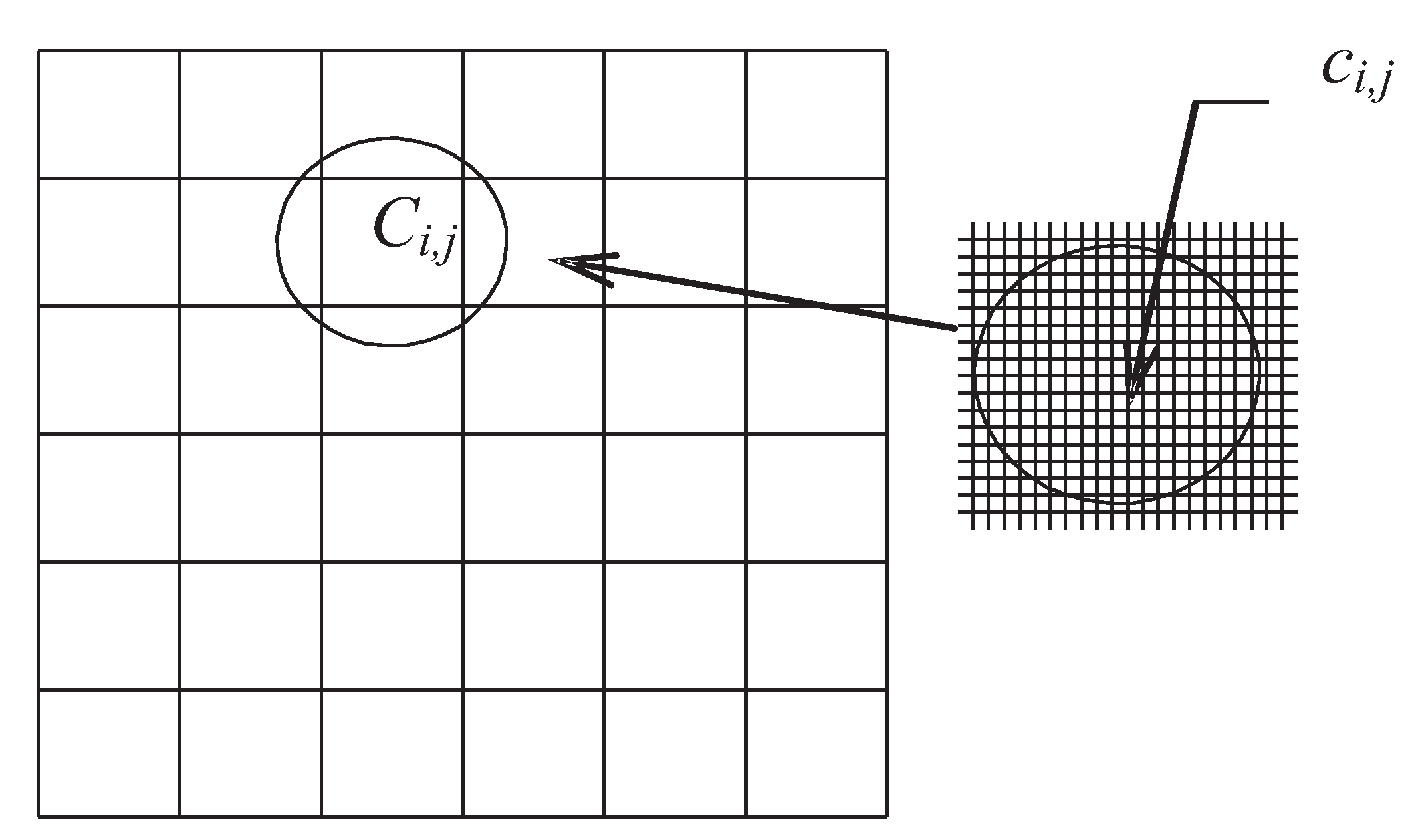
Single-phase upscaling refers to the process of upscaling permeability from the pressure Equation (1) in order to represent the properties of a fine-scale grid on a coarse-scale grid for subsurface flow modeling. The goal of single-phase upscaling techniques is to find homogeneous block permeabilities that produce the same total flow through each coarse grid block as would be obtained by solving the pressure equation on the underlying fine grid with the correct fine-scale heterogeneous structures. However, this can be challenging because the heterogeneities at all scales can have a significant impact on the large-scale flow pattern, and it is important to capture the impact of these heterogeneous structures in order to obtain a accurate coarse-scale model. To achieve this, the fine-scale Equations (1) and (2) can be replaced with a coarse-scale equation characterized by an effective permeability tensor (denoted by ${\mathbf{K}}^{\ast }$) that varies on the coarse scale, see Figure 1. This tensor represents the ability of the porous material to transmit a fluid and is an important factor in subsurface flow modeling, i.e.,

$$\nabla ·\left(-{\mathbf{K}}^{\ast }(X,Y)·\nabla p\right)=0$$

(5)

This equation sates that the net flow-rate is related to the average pressure gradient through an upscaled Darcy law.

3. Classification of Upscaling Methods

There has been ongoing research to develop new algorithms for calculating the effective properties of fluid flow in subsurface reservoirs, and a variety of techniques have been developed for this purpose. These techniques can be broadly classified into analytical methods, which use mathematical techniques to calculate the effective properties, and numerical methods, which use computational techniques to solve the underlying equations. Some of the techniques that have been developed include simple methods like arithmetic, geometric, and harmonic averages, as well as more complex tensor methods like diagonal and full tensor methods. Some of these algorithms are publicly available, while others are commercially available and may be used in reservoir simulation software. In addition to these methods, it is also possible to generate pseudo functions, such as pseudo relative permeability and capillary pressure, based on reservoir simulation of the fine grid model [11].

There are different ways to classify the upscaling methods. This classification can be done on the basis of types of parameters that are upscaled (e.g., single or two-phase flow parameters) and the methods that are used to compute these parameters (e.g., using local or global calculations) [21]. In this paper we are interested in the latter classification, i.e., the one which is related to the methods used for computing the upscaled parameters (single or two-phase). Also within the parameter upscaling classification, upscaling could be either defined as analytical or numerical upscaling. Analytical upscaling as the name suggests, is related to mathematical averaging methods, whereas, numerical upscaling relates to flow based averaging methods, which make use of underlying numerical methods to find the average permeability values. In all cases, the intent of the upscaling procedure is to replace the fine model with a coarse model. A brief overview of some of these methods is presented in this section.

3.1. Analytical Upscaling

Several analytical upscaling methods currently exist ranging from from arithmetic averaging to power law techniques, for more detail please see [7]. One of the most effective analytical upscaling method is harmonic averaging. Harmonic averaging takes into account impact of internal no-flow boundary conditions, which is not possible to capture using arithmetic averaging methods. Mathematically harmonic averaging is expressed as follows:

$$K^{\ast }=n/(1/K_1+1/K_2+\dots \dots +1/K_n)$$

(6)

Although harmonic upscaling methods are most effective, they are limited to isotropic permeability tensor only. And therefore are limited in application to text book examples only.

3.2. Numerical Upscaling

There are several numerical methods that can be used to upscale the fine-scale permeability tensor to a coarser scale for subsurface flow modeling. These methods can be broadly classified into two categories: diagonal methods and full tensor methods. The choice of method can depend on factors such as the underlying fine-scale permeability tensor, the grids being used, and the boundary conditions for the numerical method [21].

Diagonal methods involve calculating the effective permeability in each direction independently, assuming that the permeability is isotropic in that direction. These methods are relatively simple and computationally efficient, but may not be as accurate as full tensor methods in representing the anisotropic nature of the permeability tensor [21].

Full tensor methods, on the other hand, involve calculating the full effective permeability tensor, which includes all components of the tensor and can account for anisotropy. These methods are more accurate than diagonal methods, but may be more computationally expensive [21].

Both diagonal and full tensor methods can be useful depending on the specific needs and constraints of the problem being modeled. It is important to carefully consider the trade-offs between accuracy and computational cost when choosing an upscaling method.

A standard numerical approach for upscaling the permeability tensor with Equation (5) involves determining the geometry of fine-scale cells, followed by the application of appropriate pressure drop and boundary conditions in a particular direction to estimate the effective permeability tensor. One of the significant issues that arises at this stage is the choice of appropriate boundary conditions to be imposed. One option is to use global pressure gradient boundary conditions, in which a pressure gradient is applied across the cell in a specific direction (e.g., the x-direction) and no-flow boundary conditions are applied on the top and bottom boundaries of the cell, Figure 2. These boundary conditions require solving the Equation (5) for upscaling the permeability tensor twice. Other possible boundary conditions include imposing a fixed pressure or flow rate on one or more boundaries of the cell, or using periodic boundary conditions. The choice of boundary conditions can affect the accuracy and computational cost of the upscaling method, and it is important to carefully consider these trade-offs when selecting boundary conditions.

In the first solution we have following equations:

$$\begin{array}{ccc}\hfill p(0,y)& =& 1\hfill \end{array}$$

(7)

$$\begin{array}{ccc}\hfill p(L_x,y)& =& 0\hfill \end{array}$$

(8)

$$\begin{array}{ccc}\hfill v(x,0)·\left({\mathbf{n}}_{\mathbf{1}}\right)& =& v(x,L_x)·\left({\mathbf{n}}_{\mathbf{2}}\right)=\mathbf{0}\hfill \end{array}$$

(9)

In the second solution we have following equations:

$$\begin{array}{ccc}\hfill p(x,0)& =& 1\hfill \end{array}$$

(10)

$$\begin{array}{ccc}\hfill p(x,L_y)& =& 0\hfill \end{array}$$

(11)

$$\begin{array}{ccc}\hfill v(0,y)·\left({\mathbf{n}}_{\mathbf{1}}\right)& =& v(L_x,y)·\left({\mathbf{n}}_{\mathbf{2}}\right)=\mathbf{0}\hfill \end{array}$$

(12)

While in the second solution the pressure difference is specified to be in the y direction. This upscaling procedure gives us an effective diagonal permeability tensor. Using the above pressure and velocity boundary condition upscaled permeability $K^{\ast }$ determined by global mass conservation conditions is given as

$$-K_{11}^{\ast }\frac{(p(0,y)-p(L_1,y))L_2}{L_x}=-\sum _{i=1}^{ny}\frac{(p_{i+1,j}-p_{i,j})K_{i+1/2,j}\Delta y}{\Delta x}$$

(13)

where pressure differential in x-direction on upscaled grid is compared with pressure differential in x-direction on fine scale grid. The boundary conditions can then be interchanged between x and y to find the upscaled permeability in other direction

$$-K_{22}^{\ast }\frac{(p(x,L2)-p(x,0))L_1}{L_y}=-\sum _{j=1}^{nx}\frac{(p_{i,j+1}-p_{i,j})K_{i,j+1/2}\Delta x}{\Delta y}$$

(14)

The Equations (13) and (14) represent the equivalent permeabilities in the x-direction ($K_{11}^{\ast }$) and y-direction ($K_{22}^{\ast }$) respectively. Because of the no-flow boundary condition, there is no cross-flow over the domain, which results in the equivalent permeability tensor being diagonal and cross-terms $K_{12}^{\ast },K_{21}^{\ast }$ being equal to zero. However, for non-K-orthogonal grids, the cross-terms can be significant, requiring the use of full tensor upscaling methods. The standard no-flow boundary condition used in upscaling is consistent with the harmonic average approximation in the presence of a one-dimensional permeability field.

Periodic boundary conditions are a popular option for upscaling the permeability tensor using numerical methods. With these boundary conditions, each grid block is assumed to be a periodic cell in a periodic medium, and full correspondence is imposed between the pressure and velocities at opposite sides of the block. Periodic boundary conditions have several useful features, including the fact that they guarantee that the resulting effective permeability tensor $K^{\ast }$ will be symmetric and positive definite, which means that post-processing of the results is not required to ensure these properties. This can be a useful feature in situations where the symmetry and positive definiteness of the permeability tensor are important for the accuracy of the model. However, it is important to note that periodic boundary conditions may not be appropriate in all cases, and it is necessary to carefully consider the trade-offs between accuracy and computational cost when choosing boundary conditions for upscaling the permeability tensor.

3.3. Local Upscaling Methods

Local upscaling methods are a type of numerical upscaling technique that involve calculating coarse-scale parameters by considering only the fine-scale region corresponding to the target coarse block. No additional fine-scale information is included in the upscaling calculation. In these methods, each local problem is solved one at a time, with one coarse block being associated with one fine block, as shown in Figure 3. The upscaled permeability values are then computed over each coarse block. Local methods are generally quite fast computationally, but they can lack accuracy if the boundary conditions chosen for solving the local upscaling problems are not appropriate. It is important to carefully consider the trade-offs between accuracy and computational cost when choosing an upscaling method, and to select the method that is most appropriate for the specific needs of the problem being modeled.

3.4. Global Upscaling Methods

In a global upscaling technique, the entire fine scale model is simulated for the calculation of the coarse scale parameters. Here, the coarse scale parameters are assumed to be applicable to other (related) flow scenarios. Global system is solved subjected to a boundary condition (Figure 4) and upscaled parameters are computed. In highly heterogeneous models, a significant fraction of these transmissibilities may be negative. Therefore, iteration continues until all transmissibilities are positive and there is an adequate level of agreement between the fine and coarse solutions. The global methods of upscaling have potentially high accuracy and they can guarantee very high degree of coarsening as well. These methods can provide very accurate results for a particular set of wells and boundary conditions. However, they prove to be computationally expensive because of their need for information about global solution. Robustness is also an issue associated with global methods with respect to some boundary conditions and well arrangements [3,14].

3.5. Extended Local Upscaling Methods

In extended local methods, coarse scale parameters are computed by taking into account both the target coarse block and a fine scale “border region” around it, as depicted in Figure 5. The coarse scale quantities are obtained by averaging the fine scale solution (e.g., pressure and velocity) over just the target coarse block. The figure shows the fine grid represented by finer lines, the coarse grid by heavier lines, and the shaded block is the target cell for which ${\mathbf{K}}^{\ast }$ is to be calculated. The size of the extended/border region is specified by the parameter r, which determines the number of coarse cell rings composing the border region. The extended local solution covers all the fine cells corresponding to the target cell and its border regions. The region shown in Figure 5, which corresponds to r = 1, is appropriate for permeability upscaling. Any boundary condition can now be applied to the expanded domain shown in the figure. The advantage of using extended local methods is that it reduces the impact of the assumed boundary conditions in upscaling, resulting in improved coarse scale description compared to purely local methods. However, these methods may not be reliable in media with high discontinuities or geology with channelized systems.

3.6. Quasi Global or Local-Global Upscaling Methods

Quasi global methods are a type of numerical upscaling technique that involve using global flow data to inform the upscaling process, although this information is only approximate. In the case of quasi global two-phase parameter upscaling, for example, the global flow field might be estimated from a single solution of the single-phase pressure equation rather than by a more computationally expensive transient solution of the two-phase flow equations. The main idea of quasi global methods is to use global coarse-scale simulations to estimate the boundary conditions that should be used in extended local methods for calculating transmissibilities. This process is iterated until the upscaled quantity is consistent with the global flow. The main advantage of quasi global methods is that they are self-consistent and use realistic boundary conditions, which can lead to improved accuracy. However, the need for a fine-scale simulation for the global flow scenario and the iterative nature of the self-consistency process can make these methods computationally expensive.

3.7. Upscaling in Digital Rock Physics

An insight into the arrangement of subsurface pore networks can be achieved through the examination of scanned sections and volumes of core samples. This is done using Digital Rock Physics (DRP), which employs digital volumes, obtained from tools such as micro computed tomography (microCT) or scanning electron microscope (SEM), to determine the properties, like porosity and permeability [34,35]. Since DRP operates at the pore-scale, it’s essential to upscale the properties to the reservoir scale for a comprehensive reservoir characterization. Machine learning algorithms can be utilized for this purpose, as demonstrated by [36], who used classification of images into various textures to upscale the properties. A machine learning technique was employed to identify texture spatial locations and subsets were created, which were then scanned at high resolutions to calculate porosity and permeability for each texture subset. These properties were then incorporated into a coarse model [22]. Another approach involves using Convolutional Neural Networks (CNNs) and downsampling methods to upscale permeability values [37]. Thus, these techniques and approaches have proven to be valuable tools in the field of reservoir characterization.

Finally, the topic of upscaling itself and the use of different types of numerical methods for upscaling along with the choices of different types of boundary conditions have been extensively presented in literature. The intent of this paper is not to provide a comprehensive review of upscaling but to explore neural upscaling method instead as an alternative upscaling technique. Therefore, it is recommended that for a complete overview of existing upscaling techniques that are applied in reservoir simulation one can refer to published literature e.g., [3,7,19,21].

4. Need for Neural Upscaling

Although analytical and numerical methods have been around for a long time, they are often not very accurate when applied to heterogeneous permeability distribution. Analytical upscaling methods are only accurate for layered or homogeneous medium, whereas numerical upscaling methods have higher accuracy and could be applied to different geological heterogeneities, but suffers from higher computational costs because the process involves solving series of small scale Darcy flow problems, which could quickly become computationally expensive depending on grid dimensions/size of computational domain, particularly for three-dimensional domains. Whereas, online computational costs are much better with neural networks. Another main drawback of numerical upscaling methods is the choice of boundary conditions having a major impact on the results. The most important limitation of the two methods is that neither of them account for uncertainty in geological heterogeneity and its impact on the upscaled permeabilities. Pros and cons of each of the analytical and the numerical upscaling methods is covered in great detail by authors of the publications [8,21].

In recent years, there has been a significant growth in the development of machine learning models with applications to subsurface fluid flow. New surrogate models have been proposed as alternatives to conventional numerical simulations [38,39,40]. A comprehensive review of machine learning applications for porous rock modeling is presented in [41]. Additionally, machine learning methods have been used to solve ordinary differential equations using neural networks [25], whereas deep learning framework has been developed to solve even partial differential equations [42]. Neural networks have been used for solving steady state and turbulent flow problems [26,27] and some other deep learning methods have also been implemented for solving poro-elastic problems in porous media [28]. The power of deep learning techniques, like RNN-LSTM type models, have also been used by researchers for history matching and forecasting of hydrocarbon flows in heterogeneous porous media [29].

Geological uncertainty is the most important parameter in reservoir simulation and this is where the most benefit could potentially come from the application of machine learning. Finding upscaled permeability and other geological properties is essentially an inverse problem, which needs to be solved until accurate results are obtained. Machine learning algorithms are well suited for solving inverse problems and our aim in this study is to use this algorithm to predict the reservoir properties. Application of data driven machine learning approach to solve the upscaling problem for homogeneous and heterogeneous porous media is the novelty of this work.

5. Neural Upscaling

Neural upscaling method described in this section refers to a new class of upscaling method where the upscaling is performed with the help of a trained a neural network, such that the upscaled permeability ${\mathbf{K}}^{\ast }$ is given as:

$${\mathbf{K}}_{\mathbf{upscaled}}^{\ast }=\mathbf{NN}({\mathbf{K}}_{\mathbf{finescale}},\mathbf{n})$$

(15)

where $\mathbf{NN}$ refers to a neural network, $\mathbf{K}$ refers to fine scale permeability and $\mathbf{n}$ refers to the level of coarsing/upscaling being asked for from the network.

For this purpose, a function fitting multilayered neural network with hidden layers of different sizes is used for training using back-propagation. The multilayered feed-forward network could be used for training of function approximation (nonlinear regression) or for pattern recognition. Once the network weights and biases are initialized, the network can be used for forecasting/pediction. The training process requires a large set of samples for capturing network behavior through inputs and targeted output samples.

The process of training a neural network involves tuning the values of the weights and biases of the network to optimize network performance, which is defined through the network performance function. The default performance function for feed-forward networks is mean square error mse the average squared error between the network outputs and the target outputs and is defined as follows:

$$F=\mathit{mse}=\frac{1}{N}\left\{{\mathrm{\Sigma }}_{i=1}^N{\left(erro{r}_i\right)}^2\right\}=\frac{1}{N}\left\{{\mathrm{\Sigma }}_{i=1}^N{(t_i-a_i)}^2\right\}$$

(16)

where N is the number of total samples, t—is the target input of the network and a—is the trained network output. In the Neural upscaling target function t is the numerically upscaled permeability. And a is the output upscaled permeability from the network. Input training also includes the several fine scale realizations, see Figure 6 for clarification on the workflow.

The network could be trained either using batch mode training or incremental training mode. The deep learning MATLAB [43] (Version 2022a) toolbox used in this work with batch training model as it is significantly faster and results in smaller errors. For training multilayered feed-forward networks, any standard numerical optimization algorithm can be used to optimize the performance function, but there are a few key ones that have shown excellent performance for neural network training. These optimization methods use either the gradient of the network performance with respect to the network weights, or the Jacobian of the network errors with respect to the weights.

The gradient and the Jacobian are calculated using a technique called the backpropagation algorithm, which involves performing computations backward through the network. The backpropagation computation is derived using the chain rule of calculus and the details of the method are described in [44].

As an illustration of how the training works, consider the simplest optimization algorithm gradient descent. It updates the network weights and biases in the direction in which the performance function decreases most rapidly, the negative of the gradient. One iteration of this algorithm can be written as:

$${\mathbf{x}}_{\mathbf{i}+\mathbf{1}}={\mathbf{x}}_{\mathbf{k}}-{\mathbf{a}}_{\mathbf{k}}{\mathbf{g}}_{\mathbf{k}}$$

(17)

where ${\mathbf{x}}_{\mathbf{k}}$ is a vector of current weights and biases, ${\mathbf{g}}_{\mathbf{k}}$ is the current gradient, and ${\mathbf{a}}_{\mathbf{k}}$ is the learning rate. This equation is iterated until the network converges. For this paper network is trained using scaled conjugate gradient algorithm.

A sample of the neural network with hidden layers and its sizes is, used in this work, shown in Figure 7. The network takes series of realization of fine scale permeability, as appended row vector, as input (it could be 256 × 256 or 128 × 128 or 64 × 64 reshaped into a row vector). And output vector consist of a series of coarse/upscaled permeabilities as row vector.

N hidden layer different sizes are used for training using function like Scaled Conjugate Gradient. Initially the input, output and output layers sizes are decided based on the input (fine scale) and output (upscaled) permeability field.

5.1. Training Data Set Generation

Although the network architecture is simple, the results of high accuracy are produced thanks to large training data set. The network is given a large number of 2-D permeability distribution as input data set, which are generated using Perlin noise function [45] on a specified grid dimension. And the output data comprises of large number of upscaled permeability distribution, corresponding to the input permeability field, generated using numerical upscaling method described in the section Numerical Upscaling. A sample subset of input (fine scale permeability distribution) and output (upscaled permeability distribution) data used for training the network is shown in Figure 8 and Figure 9 respectively. Close to 100 such input and output distributions were used for training the network. These inputs represent different geological realizations, which might exist in the subsurface.

5.2. Network Training

Next we divide the data-set into training testing and evaluation data-set. Out of the total input and output data 80% is used for the training and 20% is used for testing purposes. The Neural upscaling network regression results for training, testing, validation and overall fit shown in Figure 10. As a measure of the network’s accuracy it can be seen that a very good fit is obtained with value of R, a measure of regression fit, close to 1 for training, testing, validation and overall fit.

5.3. Network Training Parameters

Training was carried out using a network with 3 hidden layers, with each layer comprising of 30, 20 and 10 neurons (plus biases) respectively. A total of 1000 permeability realizations were used for training the network for each upscaling case. The network training involved a split of data into 80 percent for training a model a total of 1000 epochs were used. Initial learning rate of 0.001 was assigned to the model with a batch size of 20. A snapshot of training is shown in Figure 11.

6. Neural Upscaling Results

This section presents the upscaling results obtained using the neural upscaling method for various test cases. Initially validation of the neural upscaling method is performed on layered permeability field in 2D for which the analytical solution is known to be exact. These layered examples help to benchmark the neural upscaling method against the known exact analytical methods. Following which more complex heterogeneous upscaling cases are presented.

6.1. Neural Upscaling—Layered Medium

In this section, we will first present a few test cases to benchmark the neural upscaling technique against standard analytical and numerical upscaling methods. This benchmarking can be done by comparing the neural upscaling method with the analytical and numerical upscaling methods, for the cases where the methods are known to produce precise results. Initially, two test problems of single-phase Darcy flow will be considered over a square 2-D domain. For these examples, the fine-scale permeability has a layer cake structure. Analytical upscaling methods have known solution for layered medium given by arithmetic or harmonic averaging. For numerical upscaling, local flow simulations will be performed over the local fine blocks to obtain upscaled coarse block permeability of the square domain, for details see [7]. For the Neural upscaling method, series of layered cake test medium are used for training the network using the approach already described in this paper. The first test case is of a layer cake type permeability distribution with flow taking place along the direction of the layers, Figure 12a. Whereas, in the second test case the flow is perpendicular to the direction of the layers, Figure 12b.

The analytical upscaled permeability for the first test case, where the flow is along the layers, is equal to the arithmetic mean i.e., $K^{\ast }=(K_1+K_2+K_3)/3$. Whereas, for the second test case, where the flow is across the layers, it is equal to the harmonic mean, i.e., $K^{\ast }=3/(1/K_1+1/K_2+1/K_3)$. In the numerical upscaling, the boundary conditions are set as no-flow at the top and bottom with fixed pressure at the left and right sides of the domain, creating a pressure gradient of 1. $K_1$ = 1 MD, $K_2$ = 10 MD and $K_3$ = 1 MD. A comparison of the upscaled permeability obtained via the analytical, the numerical upscaling and the neural upscaling techniques is presented in

Table 1. A comparison of the upscaled permeability values obtained using analytical, numerical and neural upscaling methods. The results are in close agreement for both the test cases.

Upscaling	${\mathit{K}}_{\mathbf{analytical}}^{\ast }$	${\mathit{K}}_{\mathbf{numerical}}^{\ast }$	${\mathit{K}}_{\mathbf{neural}}^{\ast }$
Case 1	$(K_1+K_2+K_3)/3=4.000$	$<u>/\nabla p=4.000$	$\mathbf{NN}(\mathbf{K},\mathbf{n})=\mathbf{4}.\mathbf{000}$
Case 2	$3/(1/K_1+1/K_2+1/K_3)=1.4826$	$<u>/\nabla p=1.4826$	$\mathbf{NN}(\mathbf{K},\mathbf{n})=\mathbf{1}.\mathbf{4826}$

. It should be noted that for these test cases since the underlying fine scale permeability tensor is isotropic therefore the upscaled permeability tensor is also isotropic. Results clearly show that the neural upscaling procedures give exactly same results as the analytical and the numerical upscaling technique for these test cases.

Next, we perform similar comparison for a 2-D example of layered permeability field on a fine grid of 128 × 128 grid cells, which is then upscaled using numerical and neural upscaling method. The input permeability distribution is shown in Figure 13a, the numerically upscaled permeability field on a grid of 64 × 64 grid cells is shown in Figure 13b and the neural upscaled permeability field on a grid of 64 × 64 grid cells is shown in Figure 13c. For neural upscaling the model is trained on a series of data-sets with layered permeability field as input and numerically upscaled permeability as output. The neural upscaled permeability is then compared against the numerically upscaled permeability values and it can again be seen from the results that neural and numerical upscaling gives exactly the same results.

6.2. Neural Upscaling—Heterogeneous Medium

Next, we perform upscaling on a heterogeneous channel type permeability distribution. Initially a large data-set of 2D channel type permeability distribution is generated for training the network using Perlin noise function. The network is trained until the regression fit is close to 1, Figure 14 shows the input and output target images along with outcomes of network training for the case where upscaling is performed using a factor of 2.

Once the network is training is complete a typical permeability distribution on a fine mesh is generated using Perlin noise function is given as input to the Neural upscaling network. The Neural upscaling is then performed using the trained network. The fine scale permeability distribution along with numerically upscaled permeability on a coarse mesh obtained using no-flow boundary condition is shown in Figure 15a,b. The neural upscaled permeability is shown in Figure 15c. The regression fit for the training, testing and validation is shown in Figure 15d and error measure is shown as a log plot of difference between numerical and neural upscaling results in Figure 15e. It can be seen from the log error plot that the differences are very small. From image of the neural upscaled permeability it can be seen that the channeled heterogeneity is very accurately captured and is comparable to the numerical upscaling results.

6.3. Neural Upscaling—Successive Re-Normalization

Next, successive upscaling is performed on a heterogeneous channel type permeability distribution using neural upscaling method. The local permeability is hierarchically upscaled to the next coarse grid level, re-normalizing the permeability values to each coarser level. In this case the fine scale permeability is initially upscaled by a factor of 2 and then followed by a factor 4. The objective here is to test impact of successive upscaling on the quality of upscaled permeability field. The results are compared with equivalent permeability obtained from numerical upscaling. The results are shown in Figure 16.

6.4. Sensitivity Analysis

Next, a sensitivity analysis is carried out to test the impact of network parameters on the upscaling results. Here we perform two types of sensitivity analysis. First experiment is related to changing the network architecture by changing the number of layers and keeping input training data same for both networks. Second by changing the amount of input data for same network architecture. The results for the first set of sensitivity are shown in Figure 17. In this case network architecture is changed from 4–6 hidden layers. With each added layer no. of neurons increased by 10. We can see from the results that adding additional number of layers and neurons does not have a significant impact on the results. For the second case the amount of data used for training is successively increased by a factor of 10. The improved regression fit is obtained as expected, see Figure 18. The test demonstrates that results are more sensitive to the total data compared to the number of hidden layers.

6.5. Neural Upscaling—Impact on Flow

Finally, we demonstrate that the upscaled permeability, obtained using neural upscaling, is able to reproduce flow and pressure profiles similar to the one generated using fine scale and numerically upscaled permeability. Figure 19 presents the results of this demonstration. Figure 19a shows the fine scale permeability on 128 × 128 × 1 grid, fine Scale pressure and saturation Profiles for Quarter-5-spot pattern injection. Figure 19b shows the numerically upscaled permeability on 64 × 64 × 1 grid, Upscaled pressure and saturation Profiles for Quarter-5-spot pattern injection. Figure 19c shows the neural upscaled permeability on 64 × 64 × 1 grid, upscaled pressure and saturation Profiles for Quarter-5-spot pattern injection. It can be seen that neural upscaling results are comparable to numerically upscaled results.

7. Summary and Conclusions

In this paper the details of constructing a Neural network for tackling upscaling problem is presented, referred to as Neural upscaling.

• The Neural upscaling method is developed using a feed-forward neural network with fully connected hidden dense layers, and is trained using automatic differentiation through a process called backpropagation.
• Paper also presents a study using the Neural upscaling method. Series of upscaling tests are performed on cases involving varying degree of fine scale permeability heterogeneity. A self consistent study is performed where stochastically generated $Perlin$ field [45], which mimics the subsurface permeability distribution and heterogeneity, is used for each grid level including the reference solution. Mean square error is used a parameter to optimize network performance with the help of a large training data-set comprising of over 100 realizations of permeability distribution. Equivalent upscaled permeability is used as a measure of the performance of the neural upscaling method in comparison to numerical and analytical upscaling methods. Error estimates between Numerical upscaling and Neural upscaling are also obtained. Results for various test cases that mimic the 2D permeability distribution are presented.
• Sensitivity to network layers and number of neurons is also performed, which indicates that minimum 4 hidden layers are needed to achieve a reasonably good upscaled permeability with minimum errors.
• Sensitivity analysis also shows that results are sensitive to the total data set used for training more compared to number of hidden layers of the neural network architecture.
• Although the neural upscaling method is a new approach to upscaling, it has one limitation. The need for large amount of training data. In this paper Pseudo training data has been generated using classical upscaling approach.

References

1. Christie, M.A. Upscaling for reservoir simulation. J. Pet. Technol. 1996, 48, 1004–1010. [Google Scholar] [CrossRef]
2. Christie, M.A.; Blunt, M.J. Tenth spe comparative solution project: A comparison of upscaling techniques. SPE Reserv. Eval. Eng. 2001, 4, 308–317. [Google Scholar] [CrossRef]
3. Durlofsky, L.J. Durlofsky, L.J. Numerical calculation of equivalent grid block permeability tensors for heterogeneous media. Water Resour. Res. 1991, 27, 699–708. [Google Scholar] [CrossRef] [Green Version]
4. Pal, M. Families of Control-Volume Distributed cvd(mpfa) Finite Volume Schemes for the Porous Medium Pressure Equation on Structured and Unstructured Grids. Ph.D. Thesis, University of Wales, Swansea, UK, 2007. [Google Scholar]
5. Pal, M.; Edwards, M.G. The competing effects of discretization and upscaling—A study using the q-family of CVD-MPFA. In Proceedings of the ECMOR 2008—11th European Conference on the Mathematics of Oil Recovery, Bergen, Norway, 8–11 September 2008. [Google Scholar]
6. Pal, M. A unified approach to simulation and upscaling of single-phase flow through vuggy carbonates. Int. J. Numer. Methods Fluids 2012, 69, 1096–1123. [Google Scholar] [CrossRef]
7. Pal, M.; Edwards, M.G. The effects of control-volume distributed multi-point flux approximation (CVD-MPFA) on upscaling—A study using the CVD-MPFA schemes. Int. J. Numer. Methods Fluids 2012, 68, 18–35. [Google Scholar] [CrossRef]
8. Renard, P.; de Marsily, G. Calculating equivalent permeability: A review. Adv. Water Resour. 1997, 20, 253–278. [Google Scholar] [CrossRef] [Green Version]
9. King, P.R. The use of renormalization in calculating effective permeability. Transp. Porous Media 1989, 4, 37. [Google Scholar] [CrossRef]
10. Pal, M.; Edwards, M.G. Effective upscaling using a family of flux-continuous, finite-volume schemes for the pressure equation. In Proceedings of the ACME 06 Conference, Queens University Belfast, Northern Ireland, UK, Belfast, UK, 19 April 2006; pp. 127–130. [Google Scholar]
11. Barker, J.W.; Thibeau, S.A. A critical review of the use of pseudorelative permeabilities for upscaling. SPE Reserv. Eng. 1997, 12, 138–143. [Google Scholar]
12. Arnes, J.E. On the use of mixed multiscale finite element method for greater flexibility and increased speed or improved accuracy in reservoir simulation. Multiscale Model. Simul. 2004, 2, 421–439. [Google Scholar] [CrossRef]
13. Arnes, J.E.; Gimse, T.; Lie, K.-A. An Introduction to The Numerics of Flow in Porous Media Using Matlab. In Geometrical Modeling, Numerical Simulation, and Optimization: Industrial Mathematics at SINTEF; Springer: Berlin/Heidelberg, Germany, 2007. [Google Scholar]
14. Alpak, F.O.; Pal, M.; Lie, K.-A. A multiscale adaptive local-global method for modelling flow in stratigraphically complex reservoirs. SPE J. 2012, 17, 1056–1070. [Google Scholar] [CrossRef]
15. Chen, Z.; Hou, T.Y. A mixed multiscale finite element method for elliptic problems with oscillating coefficients. Math. Comp. 2003, 72, 541–576. [Google Scholar] [CrossRef] [Green Version]
16. Chen, Y.; Durlofsky, L.J.; Gerritsen, M.; Wen, X.H. A coupled local-global upscaling approach for simulating flow in highly heterogeneous formations Adv. Water Resour. 2003, 26, 1041–1060. [Google Scholar] [CrossRef]
17. Fatemeh, M.; Mehdi, M.D.; Morteza, D. Simulation of two-phase incompressible fluid flow in highly heterogeneous porous media by considering localization assumption in multiscale finite volume method. Appl. Math. Comput. 2021, 390, 125649. [Google Scholar]
18. Hou, T.Y.; Wu, X.H. A multiscale finite element method for elliptic problems in composite material and porous media. J. Comput. Phys. 1997, 134, 169–189. [Google Scholar] [CrossRef] [Green Version]
19. Lee, S.H.; Jenny, P.; Tchelepi, H. Multi-scale finite volume methods for elliptic problems in subsurface flow simulation. J. Comput. Phys. 2003, 187, 47–67. [Google Scholar]
20. Pal, M.; Lamine, S.; Lie, K.-A.; Krogstad, S. Validation of multiscale mixed finite-element method. Int. J. Numer. Methods Fluids 2015, 77, 206–223. [Google Scholar] [CrossRef]
21. Farmer, C.L. Upscaling: A review. Int. J. Numer. Methods Fluids 2002, 40, 63–78. [Google Scholar] [CrossRef]
22. Mohamed, S.J.; Ali, A.; Moussa, T.; Fawaz, H.; Khurshed, R. Permeability upscaling in complex carbonate samples using textures of micro-computed tomography images. Int. J. Model. Simul. 2020, 40, 245–259. [Google Scholar] [CrossRef]
23. Rezaee, R.; Ekundayo, J. Permeability Prediction Using Machine Learning Methods for the CO2 Injectivity of the Precipice Sandstone in Surat Basin, Australia. Energies 2022, 15, 2053. [Google Scholar] [CrossRef]
24. Menke, H.P.; Geiger, S. Upscaling the porosity—Permeability relationship of a microporous carbonate for Darcy-scale flow with machine learning. Sci. Rep. 2001, 11, 2625. [Google Scholar] [CrossRef]
25. Chen, R.T.; Rubanova, Y.; Bettencourt, J.; Duvenaud, D.K. Neural Ordinary Differential Equations. In Proceedings of the 32nd Conference on Neural Information Processing Systems (NeurIPS 2018), Montréal, QC, Canada, 3–8 December 2018. [Google Scholar]
26. Guo, X.; Li, W.; Iorio, F. Convulutional Neural Networks for Steady Flow Approximation. In Proceedings of the 22nd ACM SIGKDD International Conference on Knowledge Discovery and Data Mining, San Francisco, CA, USA, 13–17 August 2016. [Google Scholar] [CrossRef]
27. Wu, J.-L.; Xioa, H.; Paterson, E.G. Physics-informed machine learning approach for augmenting turbulence models: A comprehensive framework. Phys. Rev. Fluids 2018, 2, 073602. [Google Scholar] [CrossRef] [Green Version]
28. Vasilyeva, M.; Tyrylgin, A. Machine learning for accelerating effective property prediction for poroelasticity problem in stochastic media. arXiv 2018, arXiv:1810.01586. [Google Scholar]
29. Pal, M. On application of machine learning method for history matching and forecasting of times series data from hydrocarbon recovery process using water flooding. Pet. Sci. Technol. 2021, 39, 519–549. [Google Scholar] [CrossRef]
30. Andrianov, N. Upscaling of two-phase discrete fracture simulations using a convolutional neural network. Comput. Geosci. 2022, 26, 1237–1259. [Google Scholar] [CrossRef]
31. He, X.; Santoso, R.; Hoteit, H. Application of Machine-Learning to Construct Equivalent Continuum Models from High-Resolution Discrete-Fracture Models. In Proceedings of the International Petroleum Technology Conference, Dhahran, Saudi Arabia, 13 January 2020. [Google Scholar]
32. He, X.; Santoso, R.; Alsinan, M.; Kwak, H.; Hoteit, H. Constructing Dual-Porosity Models from High-Resolution Discrete-Fracture Models Using Deep Neural Networks. In Proceedings of the SPE Reservoir Simulation Conference, Galveston, TX, USA, 4–6 October 2021. [Google Scholar]
33. He, X.; Santoso, R.; Alsinan, M.; Kwak, H.; Hoteit, H. Fracture Permeability Estimation Under Complex Physics: A Data-Driven Model Using Machine Learning. In Proceedings of the SPE Annual Technical Conference and Exibition, Dubai, United Arab Emirate, 21–23 September 2021. [Google Scholar]
34. Andrae, H.; Combaret, N.; Dvorkin, J.; Glatt, E.; Han, J.; Kabel, M.; Keehm, Y.; Krzikalla, F.; Lee, M.; Madonna, C.; et al. Digital rock physics benchmarks—Part I: Imaging and segmentation. Comput. Geosci. 2013, 50, 26–33. [Google Scholar] [CrossRef]
35. Sharma, R.; Malik, S.; Shettar, A.S. Sensitivity of Digital Rock Method for Pore-Space Estimation to Heterogeneity in Carbonate Formations. SPE J. 2021, 26, 2914–2927. [Google Scholar] [CrossRef]
36. Jouini, M.S.; Bouchaala, F.; Ibrahim, E.; Hjouj, F. Permeability and porosity upscaling method using machine learning and digital rock physics. In Proceedings of the 83rd EAGE Annual Conference & Exhibition, Madrid, Spain, 6–9 June 2022; pp. 1–5. [Google Scholar] [CrossRef]
37. Siavashi, J.; Najafi, A.; Ebadi, M.; Sharifi, M. A CNN-based approach for upscaling multiphase flow in digital sandstones. Fuel 2022, 308, 122047. [Google Scholar] [CrossRef]
38. Guérillot, D.; Bruyelle, J. Geochemical equilibrium determination using an artificial neural network in compositional reservoir flow simulation. Comput. Geosci. 2020, 24, 697–707. [Google Scholar] [CrossRef] [Green Version]
39. Sayyafzadeh, M. Reducing the computation time of well placement optimisation problems using self-adaptive metamodelling. J. Pet. Sci. Eng. 2017, 151, 143–158. [Google Scholar] [CrossRef]
40. Tang, M.; Ju, X.; Durlofsky, L.J. Deep-learning-based coupled flow-geomechanics surrogate model for CO2 sequestration. Int. J. Greenh. Gas Control 2022, 118, 103692. [Google Scholar] [CrossRef]
41. Tahmasebi, P.; Kamrava, S.; Bai, T.; Sahimi, M. Machine learning in geo-and environmental sciences: From small to large scale. Adv. Water Resour. 2020, 142, 103619. [Google Scholar] [CrossRef]
42. Zubov, K.; McCarthy, Z.; Ma, Y.; Calisto, F.; Pagliarino, V.; Azeglio, S.; Bottero, L.; Luján, E.; Sulzer, V.; Bharambe, A. NeuralPDE: Automating Physics-Informed Neural Networks (PINNs) with Error Approximations. arXiv 2021, arXiv:2107.09443. [Google Scholar]
43. MATLAB. Version 9.10.0 (R2021a); The MathWorks Inc.: Natick, MA, USA, 2010. [Google Scholar]
44. Hagan, M.T.; Demuth, H.B.; Beale, M.H. Neural Network Design; PWS Publishing: Boston, MA, USA, 1996. [Google Scholar]
45. Perlin, K. An Image Synthesizer. Siggraph Comput. Graph. 1985, 19, 287–296. [Google Scholar] [CrossRef]
Figure 1. Permeability tensor on each fine-scale cell c i , j upscaled over each coarse-scale cell C i , j .
Processes 11 00601 g001
Figure 2. Fine scale permeability upscaling with no-flow boundary conditions.
Processes 11 00601 g002
Figure 3. Local method for upscaling conditions.
Processes 11 00601 g003
Figure 4. Global method for upscaling conditions.
Processes 11 00601 g004
Figure 5. Extended local method for upscaling conditions.
Processes 11 00601 g005
Figure 6. A conceptual plot of the neural upscaling workflow.
Processes 11 00601 g006
Figure 7. Sample neural network used for training.
Processes 11 00601 g007
Figure 8. (a) Sample input data of permeability field “a” on a 128 × 128 grid used for training the neural network. (b) Sample input permeability field “b” on a 128 × 128 grid used for training the neural network. (c) Sample input permeability field “c” on a 128 × 128 grid used for training the neural network.
Processes 11 00601 g008
Figure 9. (a) Sample output data of upscaled permeability field “a” on 64 × 64 grid generated using numerical upscaling and used in training the neural network. (b) Sample output data of upscaled permeability field “b” on 64 × 64 grid generated using numerical upscaling and used in training the neural network. (c) Sample output data of upscaled permeability field “c” on 64 × 64 grid generated using numerical upscaling and used in training the neural network.
Processes 11 00601 g009
Figure 10. (a) Figure showing the regression fit for the data. (b) Figure showing the regression fit and error estimates of the fit. (c) Figure showing regression fit for training, testing, validation and overall fit.
Processes 11 00601 g010
Figure 11. (a) Snapshot of Network Training. (b) Training Parameters conditions.
Processes 11 00601 g011
Figure 12. A layer cake-like permeability distribution with alternate layers of low permeability, shown in gray color and high permeability shown in red color, (a) with flow occurring from left to right along the layers and, (b) with flow occurring from top to bottom across the layers.
Processes 11 00601 g012
Figure 13. (a) Input layer cake permeability distribution on a 128 × 128 grid size. (b) The numerically upscaled permeability field on a grid of 64 × 64 grid cells. (c) The neural upscaled permeability field on a grid of 64 × 64 grid cells.
Processes 11 00601 g013
Figure 14. Figure showing a sample subset of input and output target permeability distribution used for the network training along with outcome of the network training.
Processes 11 00601 g014
Figure 15. (a) Input channel permeability distribution on a 128 × 128 grid size. (b) The numerically upscaled permeability field on a grid of 64 × 64 grid cells. (c) The neural upscaled permeability field on a grid of 64 × 64 grid cells. (d) Figure showing regression fit on training and testing data. (e) Figure showing log plot of error between numerically upscaled permeability and neural upscaled permeability.
Processes 11 00601 g015
Figure 16. Figure showing successive comparison of upscaling from input permeability of 256 × 256 upscaled to 128 × 128 to 64 × 64. (a,d): 256 × 256 input permeability. (b,c): 128 × 128 input permeability. (e,f): 64 × 64 input permeability.
Processes 11 00601 g016
Figure 17. Figure showing sensitivity to number of layers and neurons. Changing the no. of layers from 4, 5 to 6 with each layer having 10 additional neurons compared to previous layer. The error does not changes significantly and regression plot remains more or less the same.
Processes 11 00601 g017
Figure 18. Figure showing sensitivity to number data set used for training and testing. Total data set is increased by a factor of 10 in 3 successive cases. As expected the regression fit improves for each case with more data values for training.
Processes 11 00601 g018
Figure 19. (a) Figure showing Fine Scale Permeability on 128 × 128 × 1 grid, Fine Scale Pressure and Saturation Profiles for Quarter-5-spot pattern injection. (b) Figure showing Numerically Upscaled Permeability on 64 × 64 × 1 grid, Upscaled Pressure and Saturation Profiles for Quarter-5-spot pattern injection. (c) Figure showing Neural Upscaled Permeability on 64 × 64 × 1 grid, Upscaled Pressure and Saturation Profiles for Quarter-5-spot pattern injection.
Processes 11 00601 g019