Are Neural Networks the Right Tool for Process Modeling and Control of Batch and Batch-like Processes?

Abstract

The prevalence of batch and batch-like operations, in conjunction with the continued resurgence of artificial intelligence techniques for clustering and classification applications, has increasingly motivated the exploration of the applicability of deep learning for modeling and feedback control of batch and batch-like processes. To this end, the present study seeks to evaluate the viability of artificial intelligence in general, and neural networks in particular, toward process modeling and control via a case study. Nonlinear autoregressive with exogeneous input (NARX) networks are evaluated in comparison with subspace models within the framework of model-based control. A batch polymethyl methacrylate (PMMA) polymerization process is chosen as a simulation test-bed. Subspace-based state-space models and NARX networks identified for the process are first compared for their predictive power. The identified models are then implemented in model predictive control (MPC) to compare the control performance for both modeling approaches. The comparative analysis reveals that the state-space models performed better than NARX networks in predictive power and control performance. Moreover, the NARX networks were found to be less versatile than state-space models in adapting to new process operation. The results of the study indicate that further research is needed before neural networks may become readily applicable for the feedback control of batch processes.

1. Introduction

Increasing competition and environmental regulations, alongside the importance of batch and batch-like process operation, have impelled manufacturing industries to seek improved margins via optimization of production processes. Several valuable products, including specialty chemicals and bio-pharmaceuticals, are manufactured in a batch process, and advanced process control techniques that utilize process models are being increasingly sought to improve process operation.

All of the diverse modeling techniques can be classified into one of two distinct modeling approaches: first-principles mechanistic-based modeling, and empirical data-driven modeling. First-principles models are desired for their ability to capture the underlying mechanics of processes directly through the application of physical conservation laws, such as mass or energy balances. However, the development and maintenance of first-principles models remains challenging. As an alternative, the prevalence of historical process data has enabled data-driven modeling to emerge as an attractive alternative.

Myriad modeling methods exist for the purpose of developing models from process data. Recently, neural networks have yielded compelling results in their ability to handle human tasks, such as classification, clustering, pattern recognition, image recognition, and language processing [1]. Neural networks have particularly been shown to be successful in data classification and segmentation tasks [2,3]. The power of neural networks is evidenced by their wide application, from business and social science to engineering and manufacturing. Neural networks are useful because of their versatility, which allows them to handle non-linear and complex behavior [4]. From the above, it becomes natural to seek to apply neural networks in the context of batch process control. However, the literature remains limited in the application of neural networks toward the development of dynamic models and their use in control in general, and batch process operation in particular.

Instead of neural networks, many statistical modeling approaches are available. One statistical approach is the method of partial least squares (PLS). The PLS method requires data to be partitioned into two matrices: a block for explanatory variables (X) and a block for response variables (Y). PLS is inspired by the methods of multi-linear regression (MLR) and principal component regression (PCR). MLR maximizes the correlation between X and Y; PCR captures the maximum amount of variance in X through orthogonal linear combinations of the explanatory variables. PLS seeks to consolidate between the aims of both methods by maximizing the covariance between X and Y. PLS achieves this by first projecting the explanatory variables onto a latent variable space to remove collinearity, and then performing linear regression within that latent space [5]. PLS is desired for its ability to handle collinear data and situations in which there are fewer observations relative to the number of explanatory variables. PLS techniques can also be adapted to incorporate first-principles knowledge via appended variables to the data matrices, as calculated by first-principles equations.

An alternative statistical approach is prediction error methods (PEMs). The premise underlying these methods is to determine the model parameters by minimizing the error between measured and predicted outputs. Constraints can be readily implemented into the optimization so as to impose regularity constraints on model parameters. The advantage of PEM lies in its diverse applicability, as it can be applied to most model structures and can readily handle closed systems. The drawback is the computational cost, as PEM typically requires the solving of non-convex optimization problems.

Yet another popular statistical approach is subspace identification, which identifies state-space models from input/output data. Subspace identification methods comprise two steps. The first is to estimate either the extended observability matrix or the state trajectory sequence from a weighted projection of the row space of the Hankel matrices formed from the input/output data. The second step is to then calculate the system matrices [6]. Subspace identification methods are desirable since they are computationally tractable and inherently discourage over-fitting through the use of singular value decomposition (SVD) to estimate the model order.

Recently, artificial neural networks (ANNs) have been championed for the purpose of model identification [7]. The functional form of an ANN is a network of nodes, called neurons, whose values are calculated from a vector of inputs supplied by each neuron in the preceding layer in the network, either the input layer or a hidden layer. Each neuron is connected to all neurons in the previous layer via a weighted connection, essentially leading to a functional form with parameters. The activation in each neuron is calculated as a linear combination of the activations in the previous layer, including a bias, and is modified by an activation function of choice. Common choices for the activation function are the sigmoid, hyperbolic tangent, or rectifier functions.

The networks are trained (i.e., the parameters are determined) by minimizing a cost function with respect to the network parameters, the weights and biases relating each neuron to its preceding layer. To facilitate optimization of the network parameters, the partial derivatives of the cost function with respect to the network’s weights and biases are necessary. The requisite partial derivatives can be calculated by the widely used backpropagation algorithm, which can be conceptualized in two steps. Firstly, the training data are fed to the neural network to calculate the network’s outputs and internal activations. Secondly, the needed partial derivatives are calculated backwards, beginning from the output layer, using the chain rule from differential calculus. Finally, the calculated partial derivatives allow for optimization by such methods as gradient descent [8]. While neural networks have generally found widespread acceptance, a comparative study of neural networks with other approaches for batch process modeling and control is lacking.

In light of the above, the present study aims to address the dearth of results that compare neural networks to other data-driven control techniques for batch processes. Subspace identification, which remains a prevalent and validated modeling approach for batch process control, is used as the comparative benchmark in this work. Due to its dominance in industrial practice, model predictive control (MPC) was chosen as the framework in which the viability of neural networks for control purposes could be evaluated. The comparison between the two modeling approaches is illustrated by means of a motivating example which is presented in Section 2.1. Subspace identification and neural networks are explained subsequently in Section 2.2 and Section 2.3. Thereafter, Section 3 presents models identified and validated per both modeling approaches. Finally, Section 4 presents the closed-loop results of implementing both types of models into an MPC framework, with concluding remarks to be found in Section 5.

2. Preliminaries

In this section, we first present an example to motivate our results, followed by a review of existing subspace identification and ANN approaches.

2.1. Simulation Example

Consider a PMMA polymerization process carried out in a batch stirred tank reactor with a heating/cooling jacket. The underlying kinetic mechanism for the free radical polymerization of PMMA is given in

Table 1. Kinetic mechanism for PMMA polymerization.

Kinetic Mechanism	Chemical Formula
Initiation	$I\to 2\varphi$
	$\varphi +M\to R_1$
Propagation	$R_i+M\to R_{i+1}$
Termination by combination	$R_i+R_j\to R_{i+j}$
Termination by disproportionation	$R_i+R_j\to P_i+P_j$
Chain transfer to monomer	$R_i+M\to P_i+R_1$
Chain transfer to solvent	$R_i+S\to P_i+S$

, where I is the initiator, M is the monomer, $R_i$ is a live polymer with I monomer units, $P_i$ is a dead polymer with I units, and S is the solvent [9].

The batch reactor is charged with methyl methacrylate (monomer), AIBN (initiator), and toluene (solvent). The mechanistic model for the motivating example was adapted from [10] while making appropriate alterations as per [9,11], which are further discussed in [12]. The first-principles model, which is used as a test bed, involves nine states: the concentrations of the monomer and initiator, reactor temperature, and six moments of living and dead polymer chains. The input to the process is the jacket temperature, and the measured outputs are the reaction temperature, the logarithm of viscosity, and density. The plant model was used to generate historical data for the identification of state space and NARX network models, as well as for producing the process simulation required for model validation and MPC implementation.

2.2. Subspace Identification

Subspace identification techniques identify a linear time-invariant (LTI) state-space model. The deterministic identification problem (for a continuous process) can be described as follows: if s measurements (where s represents the length of the data) of the input $u_k\in {\mathbb{R}}^m$ and the output $y_k\in {\mathbb{R}}^l$ are available, then a model with order n can be identified in the form

$$\begin{array}{c}\hfill \begin{array}{c}\hfill x_{k+1}^d=A{x}_k^d+B{u}_k\\ \hfill y_k=C{x}_k^d+D{u}_k\end{array}\end{array}$$

(1)

where the objective is to determine the order n of this unknown system and the system matrices $A\in R^{n\times n}$, $B\in R^{n\times m}$, $C\in R^{l\times n}$, $D\in R^{l\times m}$.

We denote the measured outputs as $y^{\left(b\right)}\left[k\right]$, where k is the sampling time from when the run is initialized and b denotes the run number. Thus, the Hankel matrix is laid out as follows:

$$\begin{array}{c}\hfill Y_{1|i}^{\left(b\right)}=\left[\begin{array}{c}\\ y^{\left(b\right)}\left[1\right]& y^{\left(b\right)}\left[2\right]& \cdots & y^{\left(b\right)}\left[j^{\left(b\right)}\right]\\ ⋮& ⋮& & ⋮\\ y^{\left(b\right)}\left[i\right]& y^{\left(b\right)}[i+1]& \cdots & y^{\left(b\right)}[i+j^{\left(b\right)}-1]\end{array}\right]\forall b=1,\cdots ,nb\end{array}$$

(2)

where $nb$ is the total number of runs used for identification.

A single Hankel matrix by itself would not allow data from multiple experiments or runs to be utilized, and the simple concatenation of the outputs from all of the runs would generate a data set where the initial condition of a subsequent run is the end point of the previous run, which would also be incorrect. Therefore, when concatenating the data, it is important to generate a matrix, where this assumption is not necessary to solve for the states. This can be achieved by horizontally concatenating the Hankel matrices from each run to generate our pseudo-Hankel matrix for both the input and output variables. This pseudo-Hankel matrix for the output data is defined as follows:

$$\begin{array}{c}\hfill Y_{1|i}=\left[\begin{array}{cccc}{Y}_{1|i}^{\left(1\right)}& Y_{1|i}^{\left(2\right)}& \cdots & Y_{1|i}^{\left(nb\right)}\end{array}\right]\end{array}$$

(3)

Similarly, a pseudo-Hankel matrix for the input data can be generated. A key consideration of this approach is that horizontal concatenation of data allows for runs of varying lengths to be identified without aligning the variables. The use of these pseudo-Hankel matrices for input and output data allows for data from multiple runs to be analyzed to compute the state trajectory using any subspace identification technique, such as the deterministic method used in this approach [13]. A consequence of horizontal concatenation is that the identified state trajectories also consist of horizontally concatenated state estimates from each run, which can be represented as

$$\begin{array}{cc}\hfill {\widehat{X}}_{i+1}^{\left(b\right)}& \hfill =\left[\begin{array}{ccc}{\widehat{x}}^{\left(b\right)}[i+1]& \cdots & {\widehat{x}}^{\left(b\right)}[i+j^{\left(b\right)}]\end{array}\right]\forall b=1,\cdots ,nb\hfill \end{array}$$

(4)

$$\begin{array}{cc}\hfill {\widehat{X}}_{i+1}& \hfill =\left[\begin{array}{cccc}{\widehat{X}}_{i+1}^{\left(1\right)}& {\widehat{X}}_{i+1}^{\left(2\right)}& \cdots & {\widehat{X}}_{i+1}^{\left(nb\right)}\end{array}\right]\hfill \end{array}$$

(5)

where $nb$ is the total number of training runs used for identification. Finally, once the state trajectory matrix is determined, the system matrices can be estimated using such methods as ordinary least squares, as shown below:

$$\begin{array}{c}\hfill Y_{reg}^{\left(b\right)}=\left[\begin{array}{ccc}{\widehat{x}}^{\left(b\right)}[i+2]& \cdots & {\widehat{x}}^{\left(b\right)}[i+j^{\left(b\right)}]\\ y^{\left(b\right)}[i+1]& \cdots & y^{\left(b\right)}[i+j^{\left(b\right)}-1]\end{array}\right]\end{array}$$

(6)

$$\begin{array}{c}\hfill X_{reg}^{\left(b\right)}=\left[\begin{array}{ccc}{\widehat{x}}^{\left(b\right)}[i+1]& \cdots & {\widehat{x}}^{\left(b\right)}[i+j^{\left(b\right)}-1]\\ u^{\left(b\right)}[i+1]& \cdots & u^{\left(b\right)}[i+j^{\left(b\right)}-1]\end{array}\right]\end{array}$$

(7)

$$\begin{array}{c}\hfill \left[\begin{array}{ccc}{Y}_{reg}^1& \cdots & Y_{reg}^{\left(nb\right)}\end{array}\right]=\left[\begin{array}{cc}A& B\\ C& D\end{array}\right]\left[\begin{array}{ccc}{X}_{reg}^{\left(1\right)}& \cdots & X_{reg}^{\left(nb\right)}\end{array}\right]\end{array}$$

(8)

yielding A, B, C and D as the state-space model matrices, and are henceforth collectively referred to as the unconstrained model.

Remark 1. 

The key consideration for subspace identification of multiple data sets, as opposed to a single data set, is in the generation of the state trajectory. The risk of not using a pseudo-Hankel matrix structure through a concatenation of the data can result in a single-state trajectory for the data set, where the initial point of the next run is incorrectly linked to the end point of the previous run. The subspace identification approach allows for the correct identification of the separate state trajectories from the training data to be used for model identification, thus enabling the usage of multiple runs during training.

Notably, prior work has assessed the value of subspace identification for batch processes [14]. Subspace identification was employed to generate a data-driven state-space model for the PMMA polymerization process, being used as a test-bed for the present study. The state-space model was then implemented into MPC, and the resulting performance was compared with state-of-the-art latent variable methods. The results from their investigation demonstrated the superiority of using subspace identification for the modeling and control of batch processes. Motivated by these findings, state-space models were selected as the benchmark by which to evaluate ANNs in this work.

2.3. ANN-Based Dynamic Models

To enable the modeling of dynamical systems in ANNs, information is allowed to flow between each iteration via tapped delay lines or recurrent (feedback) connections. For instance, time delay neural networks are feedforward dynamic neural networks that allow for the inclusion of historical data via tapped delay lines.

Recurrent neural networks (RNNs), however, are more suitable for dynamic process modeling, as they encode an internal state (memory) of the system by incorporating feedback connections. Past outputs or hidden states are looped back into the neural network, thereby allowing for information to flow between each iteration of the network. Hence, the response of RNNs depends on the historical sequences of both input and output data. NARX networks, a class of RNNs involving only feedback from the output neuron, are used as a representative for this study [15]. A mathematical representation of a general NARX network is given by

$$y(n+1)=f[y\left(n\right),...,y(n-d_y);u\left(n\right),...,u(n-d_u)]$$

(9)

where $u\left(n\right)$ and $y\left(n\right)$ are the current inputs and outputs, $d_u\left(n\right)$ and $d_y\left(n\right)$ are the associated input and output delays, and $f(·)$ is a nonlinear function [16].

NARX networks are derived from the application of autoregressive exogeneous (ARX) models to the framework of artificial intelligence. Therefore, NARX networks are the artificial intelligence counterparts of ARX models, which are a mainstay of process modeling. Contrasting the two modeling approaches, it is noteworthy that far more advanced computational techniques have been developed for neural networks than exist for traditional ARX modeling. In particular, NARX networks can readily incorporate nonlinear elements via a host of different activation functions.

RNNs are able to learn temporal sequences by retaining a ’memory’ of system dynamics. However, practice reveals that RNNs are difficult to train, particularly in learning dependencies over long sequences of data [17]. The difficulties in training RNNs can be understood by looking carefully at their associated learning algorithms. To optimize the cost function, the algorithm of back propagation through time (BPTT) is used. In BPTT, the RNN is first ‘unrolled’ across a time sequence before the regular backpropagation algorithm can be used for optimization purposes. Hence, BPTT is simply a specific application of backpropagation to the learning of RNNs. Since the unrolled RNN often becomes very deep, the training of RNNs is especially complicated by the problem of exploding or vanishing gradients. For this reason, RNNs struggle to store information over extended time intervals [18].

LSTM networks have been proposed as an alternative to RNNs. LSTM networks are a class of RNNs whose architecture incorporates long-term memory over extended time intervals via the inclusion of a cell state. The cell state is updated at each time step via forget and input gates, while the hidden state (the short-term memory state of RNNs) is controlled by an output gate. LSTM networks effectively mitigate the vanishing gradient problem by maintaining constant error backpropagation via the cell state [18].

In light of the above, LSTM networks have become a popular class of RNNs for a variety of applications, such as speech recognition, translation, and language modeling. However, for the purposes of dynamic systems modeling in the framework of model-based control, the value of LSTMs remains to be established. The main advantage of LSTM networks is the ability to learn long-term dependencies in sequential data. However, for dynamic models, the output at any given time step is largely a function of recent input and output data; the contribution of historical data reaching far back in time will attenuate over lengthy time intervals. Moreover, while learning such long-term dependencies holds the promise of more nuanced modeling, the drawback remains that over-fitting is likely to remain a problem. This is one of the reasons why state-space models have become a mainstay in model-based control, as they provide simpler but stable models which are robust to over-fitting. Finally, it is noteworthy that Ref. [19] found that NARX networks outperformed long short-term memory (LSTM) networks and convolutional neural networks in predicting groundwater level forecasts. Based on these considerations, NARX networks were selected for the architectures of the ANNs in this work.

The use of ANNs in a framework of MPC has been explored in some contexts. For example, ANN-based MPC of constrained non-linear systems [20] was proposed, where the ANN was trained by minimizing a MPC cost function. An ANN-MPC formulation was also augmented with a second ANN that would adaptively update the identified model online [21]. Another approach was to design an ideal MPC, and then train LSTMs on the generated control sequences to replace the MPC framework altogether, thereby circumventing computationally expensive optimization solutions [22]. LSTMs have also been implemented for the extraction of phase-specific features in batch processes in order to decrease the overall dimensionality of the prediction scheme [23]. Moreover, LSTMS have been applied to develop reinforcement learning controllers for enhancing the performance of heating ventilation and air conditioning systems [24].

Another approach is to include first-principles knowledge of the process via weight constraints on the training of RNNs or through the pruning of neuronal connections [25]. It was demonstrated that such physics-based modifications to the RNNs resulted in an improved control performance. Similarly Ref. [26] incorporated a priori physical knowledge into RNNs to improve the RNN-based MPC performance of large-scale and complex chemical processes. The application of RNNs toward MPC despite the problem of collinear or insufficiently rich input data [27] was also recently addressed. Their proposed solution was to first use PCA to eliminate collinearity in the input space before identifying an RNN based on the uncorrelated scores.

Among recent developments in the field, Ref. [28] compared first-principles, state space, and ANN models in an economic MPC framework. The authors found that the ANNs often returned non-smooth prediction trajectories that complicated the solution of the optimization problem. In another study, Ref. [29] was able to attain optimal or near-optimal control of irrigation schedules by implementing an LSTM network in a mixed-integer MPC scheme. Their contributions warrant further exploration of ANNs for the modeling and control of processes with continuous inputs. Finally, Ref. [30] used LSTM networks to develop reduced-order state estimators for mechanistic models of high computational complexity.

Lastly, it must be noted that prior studies in the field have sought to examine the value of ANNs for batch process modeling and control. For example, Refs. [31,32,33,34,35,36,37] implemented ANNS for process modeling and control. However, past research has either failed to benchmark ANNs or compared the use of ANNs to classical proportional–integral–derivative control or first-principles mechanistic model-based control. As such, the comparison of ANNs to other data-driven modeling techniques, such as subspace-based state-space models, remains sparse in the literature, despite subspace identification-based models having been shown to be particularly effective in batch control [14]. Therefore, the present study seeks to address this gap by providing a comparison between subspace models and ANNs in the context of model-based predictive control of batch processes.

3. Model Identification

The first step in the proposed approach was to identify both (LTI) state-space models and NARX networks for the PMMA polymerization process. To facilitate a comprehensive comparison between the state-space and NARX network models, data sets were built using different input profiles. In particular, three distinct types of input profiles were used to generate the data sets from which the models were identified. The three types of input profiles were formed by implementing three different kinds of input profiles on the PMMA polymerization process. Specifically, the input profiles were as follows:

• A PI controller was used to track set-point trajectories.
• A pseudo-random binary sequence (PRBS) signal was superimposed onto the input moves generated by a PI controller.
• A PRBS signal was superimposed onto a nominal input trajectory.

A major aim of this study was to detect and compare over-fitting issues between subspace and NARX network models. To this end, two different sets of historical data were used to identify all models: data both with and without measurement noise. To generate noisy data, Gaussian noise was superimposed onto all output data. Specifically, measurement noise was generated from standard normal distributions modified by factors of 0.10 for temperature, 0.01 for log(viscosity), and 0.10 for density. Hence, each model was identified and evaluated for performance both in the presence and absence of noise. In this way, state-space and NARX network models were compared in their robustness to over-fitting issues resulting from noisy data.

The identification of ANNs is complicated by inherent randomness in the training algorithms. Randomness is introduced in the training of ANNs via random parameter initialization and sampling division, among other sources [38]. Such randomness in the training process often leads to a lack of replicability in model identification. To ensure replicability and consistency, the seed was set to a specific and definite value, thereby permitting consistent comparisons between state-space models and NARX networks. However, it is noteworthy that neural networks will often perform differently depending on the seed. A possible explanation for this observation can be the existence of multiple local minima on the surfaces of the cost function. For this reason, it has been suggested to include the seed as a hyperparameter in the identification of neural networks [39].

The models were fitted against training data, and goodness-of-fit evaluations were calculated as per the normalized root mean squared error (NRMSE) measure, given by

$$NRMSE\left(i\right)=\frac{\left|\right|y_{ref}(:,i)-y(:,i){\left|\right|}^2}{\left|\right|y_{ref}(:,i)-mean\left(y_{ref}(:,i)\right){\left|\right|}^2}$$

(10)

where y is the predicted output, $y_{ref}$ is the measured output, and i indexes the outputs. A large negative value in the NRMSE evaluation indicates a poor fit, zero indicates a perfect fit, and unity indicates that the model is no better than a straight line in explaining the variance of the data.

Three sets of historical data were generated for model identification. Each data set comprised thirty batches, ten batches for each of the three types of input profiles listed above. The first of these data sets was used as training data to identify the initial state-space models and NARX networks; the associated NRMSE calculations yielded the fit of the models. The identified models were then evaluated for predictive power against a second data set, with the NRMSE calculations being taken as an internal validation of the models. The models were then tweaked for improved performance by trial-and-error optimization of the NRMSE evaluations with respect to model parameters, for cases both with and without measurement noise.

However, the goodness of fit of a model does not preclude the possibility of over-fitting. Hence, an approach as described would be naive and insufficient for accurately assessing the predictive power of models. Consequently, it is essential to validate the models against novel data. For this reason, an additional measure of the models was calculated. In this last step, the tweaked models were validated against a third set of data. Finally, these resulting NRMSE evaluations were taken as the validation and true measures of model performance.

The procedure described above was followed in the identification of state-space models. The parameter for the number of states ($n=10$) was tuned by a brute-force search that yielded the best fit, or the best NRMSE evaluation, in comparing model predictions to training data. The lag i was set to twice the number of states. The identified state-space models were tested against the second set of data for the purpose of internal validation. The associated NRMSE calculations were used to tweak model parameters for improved performance; however, this step was found to be unnecessary for state-space models. Finally, the state-space models were validated against the last set of data; the resulting NRMSE calculations were considered the true measures of the models’ predictive power.

In the validation of state-space models, Kalman filters were used for state estimation. The equations for the Kalman filter are given in Equation (11), where $P_{k|k-1}$ is the estimated (a priori) covariance, $P_{k|k}$ is the estimated (a posteriori) covariance, and $K_k$ is the Kalman gain; Q and R, calculated as per Equation (12), are the covariance matrices for both the process and measurement noise, respectively. The two covariance matrices are taken to be time independent.

$$\begin{array}{c}\hfill \begin{array}{cc}\hfill & P_{k|k-1}=A{P}_{k-1|k-1}{A}^T+Q\hfill \\ \hfill & K_{k|k}=\frac{P_{k|k-1}{C}^T}{C{P}_{k|k-1}{C}^T+R}\hfill \\ \hfill & P_{k|k}=(I-K_{k}C)P_{k|k-1}\hfill \\ \hfill & {\widehat{x}}_{k|k-1}=A{\widehat{x}}_{k-1|k-1}+B{u}_k\hfill \\ \hfill & {\widehat{x}}_{k|k}={\widehat{x}}_{k|k-1}+K_k[y_k-(C{\widehat{x}}_{k|k-1}+D{u}_k)]\hfill \\ \hfill & {\widehat{y}}_{k|k}=C{\widehat{x}}_{k|k}+D{u}_k\hfill \end{array}\end{array}$$

(11)

$$\begin{array}{c}\hfill \begin{array}{cc}\hfill & Q=cov(X_{k+1}-\left[AB\right]{\left[X_k{U}_k\right]}^T)\hfill \\ \hfill & R=cov(Y_k-\left[CD\right]{\left[X_k{U}_k\right]}^T)\hfill \end{array}\end{array}$$

(12)

The initial state estimate was set as the zero vector, and the initial Kalman gain was set as the zero matrix. To ensure convergence, the Kalman filter was allowed to run iteratively until the absolute values of the observation error for each output fell below a threshold, as given in Equation (13). These threshold values were tuned via trial and error until acceptable convergence was achieved. The first ten data samples were discarded in all NRMSE calculations to allow for the observer to converge.

$$\begin{array}{c}\hfill \begin{array}{c}\hfill |Y_k-{\widehat{Y}}_k|<{\left[\begin{array}{ccc}0.3& 0.1& 0.5\end{array}\right]}^T\end{array}\end{array}$$

(13)

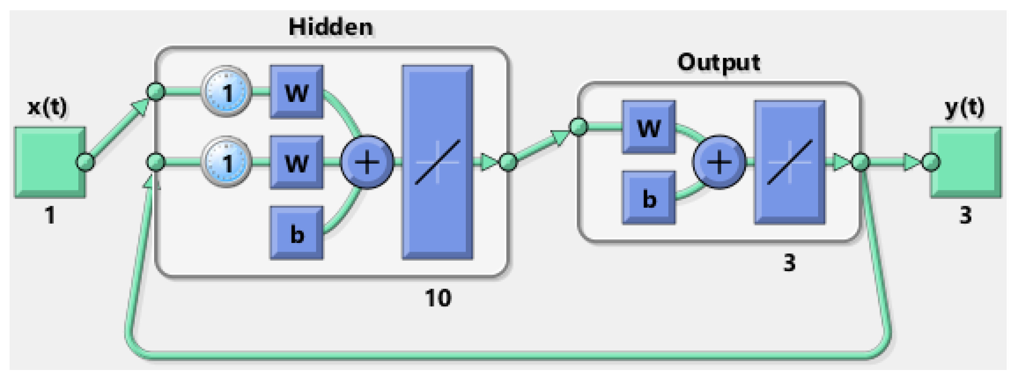
NARX networks were identified following a similar procedure as for state-space models. Firstly, the NARX networks were trained on the first set of data. In the training of all NARX networks, 70% of the input/output data were reserved for training, 15% for validation, and 15% for testing. For all NARX networks, outputs and errors were normalized within the ranges of $(-0.5,0.5)$ and $(-1,1)$ respectively. The initial, rudimentary architecture from which neural networks were developed is shown in Figure 1. The neural transfer functions, number of hidden layers, and size of the hidden layers were determined by trial and error until the best NRMSE evaluation was found.

Then, the trained networks were internally validated against a second set of input/output data; the model parameters and architectures were tweaked by a trial and error approach. Lastly, the neural networks were validated against the third and final set of data to obtain NRMSE calculations representing the true model performance of the networks. Figure 2 displays the final architecture of the neural networks identified, both in the absence and presence of measurement noise.

Notably, the first layer of the NARX network incorporates an initial nonlinear element to capture the nonlinear dynamics of the PMMA polymerization process. As discussed earlier, one of the main advantages of ANNs over state-space models is in their ability to handle nonlinearities directly. By including nonlinearity into the model, ANNs allow for the enhanced assimilation of process knowledge and thereby strive to improve predictive and control performance.

Note that while the neural networks do not require an explicitly designed observer as do state-space models, an initial fragment of the input/output data is required to initialize the NARX networks, as is the case for ARX models in general. This initial fragment of input/output data needed by NARX networks can be thought of as representing the role of a state-space observer, with the length of data reflecting the time it would take for the state-space observer to converge to an accurate state estimate.

Table 2. Mean NRMSE evaluations for the validation of the identified models.

	Temperature [K]	log(Viscosity)	Density [kg/m3]
State Space (without measurement noise)	0.19	0.08	0.08
State Space (with measurement noise)	0.23	0.08	0.10
NARX network (without measurement noise)	0.27	0.21	0.23
NARX network (with measurement noise)	0.29	0.22	0.23

tabulates the NRMSE evaluations associated with the validation of both state-space models and NARX networks. Accordingly, Figure 3 and Figure 4 display an example of the validation of state-space models and NARX networks, identified both in the absence and presence of measurement noise, respectively. The state-space models outperformed NARX networks in predictive power, as observed by the lower NRMSE evaluations for state-space models in Table 2. The data also reveal that both state-space models and NARX networks were resilient to over-fitting measurement noise since the NRMSE evaluations did not increase sharply upon incorporation of measurement noise.

To further assess model performance, the identified models were tested against a fourth set of historical plant data. For the purposes of gauging possible over-fitting, this new set of data was generated to be distinct from the three types of data sets used previously in model identification. In particular, the data set was formed via the generation of PRBS input profiles. Figure 5 contrasts between one of the input profiles used in model identification and one of the input profiles from this fourth data set.

Table 3. Mean NRMSE evaluations for the validation of the identified models against distinctly generated input trajectories.

	Temperature [K]	log(Viscosity)	Density [kg/m${}^3$]
State Space (without measurement noise)	0.20	0.13	0.09
State Space (with measurement noise)	0.20	0.14	0.12
NARX network (without measurement noise)	0.52	0.30	0.33
NARX network (with measurement noise)	0.52	0.30	0.33

tabulates the mean NRMSE evaluations associated with the plant data and model predictions. Concurrently, Figure 6 and Figure 7 present examples of prediction performance for the identified models. Here, a large performance gap is observed between the predictive power of state-space models and NARX networks, as observed by the increased difference between NRMSE evaluations between the modeling approaches. NARX networks are shown to be poor in predicting new and distinct data profiles. While the neural networks did not significantly over-fit measurement noise, as was established earlier, they did over-fit the training data. This is clearly evidenced by the worse NRMSE evaluations for NARX networks modeling input/output data that are characteristically distinct from the original training data.

4. Closed-Loop Results

Having identified both state-space models and NARX networks, the models were then implemented into MPC for forward prediction of the evolution of the PMMA polymerization process. The MPC scheme was realized by minimizing the cost function

$$\begin{array}{c}\hfill \begin{array}{cc}\hfill & J=\sum _{i=1}^{H_p}dy\left(i\right)\times Q_y\times dy{\left(i\right)}^T+du\left(i\right)\times R_{du}\times du{\left(i\right)}^T\hfill \\ \hfill & dy\left(i\right)=y\left(i\right)-y_{ref}\left(i\right)\hfill \\ \hfill & du\left(i\right)=u\left(i\right)-u(i-1)\hfill \end{array}\end{array}$$

(14)

where $R_{du}$ and $Q_y$ are positive definite weighting matrices penalizing input moves and deviation from the reference output trajectory, respectively. MPC was implemented in MATLAB using the fmincon function; iteratively, at each time step, the fmincon solver was called to solve the optimization problem for the optimal control moves.

In the case of state-space models, the MPC parameters were tuned such that $Q_y$ was set to the identity matrix, $R_{du}$ was set to the zero matrix, and $H_p=H_c=1$ was set as both the prediction and control horizons. Additionally, a Kalman filter was repeated as similar to Section 3, except that the initial state vector was now estimated using MATLAB’s findstates function from training data.

As with ARX models, it is necessary to initialize the internal states of the (closed-loop) NARX networks at each time step to allow for forward prediction. To achieve this, recent plant data were used to iteratively update the internal states of the NARX networks; this can be thought of as being analogous to how state estimation is implemented in the use of state-space models. In particular, the last 10 time steps of input/output data were used to initialize the neural network at each iteration.

In the case of neural networks, the MPC parameters were picked as follows: $Q_y=\left(\begin{array}{ccc}100& 0& 0\\ 0& 1& 0\\ 0& 0& 1\end{array}\right)$, $R_{du}=50$, $H_p=2$ was set as the prediction horizon, and $H_c=1$ the control horizon. For the first 10 time steps, the plant was allowed to operate under open-loop conditions. Then, closed-loop control was implemented using the NARX networks as predictors for the MPC. At each iteration, the last 10 time steps were used to estimate the current internal state of the neural network.

Table 4. Mean NRMSE evaluations between the control and reference trajectories.

	Temperature [K]	log(Viscosity)	Density [kg/m${}^3$]
State Space (without measurement noise)	0.49	0.61	0.56
State Space (with measurement noise)	0.56	0.61	0.56
NARX network (without measurement noise)	0.60	0.60	0.58
NARX network (with measurement noise)	1.07	0.60	0.58

compares the mean errors over all three process outputs in applying MPC using both state-space models and NARX networks. Both types of models were implemented in MPC, and several tests were run for 10 different reference trajectories, which were in turn determined from each of the three types of input profiles as from Section 3.

Errors between the control and reference trajectories were evaluated via NRMSE calculations; the means of those NRMSE calculations over all 30 implementations are given in Table 4. State-space models outperformed NARX networks in control of temperature, the output exhibiting the most nonlinear behavior; both models provided almost identical control over the other outputs. The control performance of NARX networks deteriorated more due to noisy conditions than that of state-space models. Figure 8 and Figure 9 show examples of the implementation of state-space and NARX network models in MPC.

To further assess model performance, the identified models were used to track novel reference trajectories. For the purposes of gauging over-fitting, this new set of data was generated to be distinct from the data sets used previously in model identification and validation. As discussed in Section 3, the data set was formed via the generation of PRBS input profiles. Refer back to Figure 5 to see an example comparison between one of the input profiles used in model identification and one of the input profiles from this final data set.

Table 5. Mean NRMSE evaluations between the control and distinctly generated reference trajectories.

	Temperature [K]	log(Viscosity)	Density [kg/m${}^3$]
State Space (without measurement noise)	0.05	0.01	0.00
State Space (with measurement noise)	0.18	0.02	0.01
NARX network (without measurement noise)	0.58	0.04	0.02
NARX network (with measurement noise)	0.67	0.04	0.03

tabulates the mean NRMSE evaluations associated with the plant data and model predictions. State-space models and NARX networks provided similar control performance for the viscosity and density outputs. Additionally, neither model was heavily impacted by measurement noise. However, there was a significant gap between the two modeling approaches in the control of temperature. Therefore, it is concluded that state-space models outperformed NARX networks in the control of novel reference trajectories. The data indicate that NARX networks were less versatile than state-space models in generalizing beyond the range of training data. Figure 10 and Figure 11 presents a visual comparison between the prediction performance of both modeling approaches with regards to novel data.

In comparing state-space models and NARX networks, it is worthwhile to not only compare control performance, but also computation times.

Table 6. Mean computation times, in seconds, for MPC simulations.

	Sans Noise	With Noise
State-space	20	21
NARX Network	150	152

tabulates the mean computation time it took for the MPC simulations to complete for each type of model. The total simulation time was averaged over the 30 reference trajectories that were tracked. Since the aim was to evaluate computational complexity, and not performance, $H_p=H_c=1$ was set as both the prediction and control horizons for the NARX networks in order to make fair comparisons between computation times. Judging by computation time, NARX networks exceeded the state space models in computational complexity by an order of magnitude.

5. Conclusions

The research presented aimed to explore if, in their present state, neural network-based models are a useful tool for process control. In particular, the focus of this study was to compare the efficacy of ANNs with state-space models within the framework of MPC. To this end, state-space and NARX network models were developed for a batch PMMA polymerization process. In this study, subspace-based state-space models outperformed NARX networks in predictive power and control performance. In particular, there was a sizable gap in the prediction capability and control performance with regards to adapting to novel data outside the scope of training data. The NARX networks were found to be vulnerable to over-fitting training data.

The results of this work reveal that NARX networks are worse predictors than state-space models in terms of model-based control. As such, more development is required before neural networks can become viable toward modeling and process control.

References

1. Abiodun, O.I.; Jantan, A.; Omolara, A.E.; Dada, K.V.; Mohamed, N.A.; Arshad, H. State-of-the-art in artificial neural network applications: A survey. Heliyon 2018, 4, e00938. [Google Scholar] [CrossRef] [PubMed] [Green Version]
2. Dreiseitl, S.; Ohno-Machado, L. Logistic regression and artificial neural network classification models: A methodology review. J. Biomed. Inform. 2002, 35, 352–359. [Google Scholar] [CrossRef] [PubMed] [Green Version]
3. Lavrukhin, E.V.; Gerke, K.M.; Romanenko, K.A.; Abrosimov, K.N.; Karsanina, M.V. Assessing the fidelity of neural network-based segmentation of soil XCT images based on pore-scale modelling of saturated flow properties. Soil Tillage Res. 2021, 209, 104942. [Google Scholar] [CrossRef]
4. Dave, V.S.; Dutta, K. Neural network based models for software effort estimation: A review. Artif. Intell. Rev. 2014, 42, 295–307. [Google Scholar] [CrossRef]
5. Geladi, P.; Kowalski, B.R. Partial least-squares regression: A tutorial. Anal. Chim. Acta 1986, 185, 1–17. [Google Scholar] [CrossRef]
6. Favoreel, W.; De Moor, B.; Van Overschee, P. Subspace state space system identification for industrial processes. J. Process. Control 2000, 10, 149–155. [Google Scholar] [CrossRef]
7. Hunt, K.J.; Sbarbaro, D.; Żbikowski, R.; Gawthrop, P.J. Neural networks for control systems—A survey. Automatica 1992, 28, 1083–1112. [Google Scholar] [CrossRef]
8. Nielsen, M.A. Neural Networks and Deep Learning; Determination Press: San Francisco, CA, USA, 2015; Volume 2018. [Google Scholar]
9. Rho, H.J.; Huh, Y.J.; Rhee, H.K. Application of adaptive model-predictive control to a batch MMA polymerization reactor. Chem. Eng. Sci. 1998, 53, 3729–3739. [Google Scholar] [CrossRef]
10. Ekpo, E.; Mujtaba, I.M. Evaluation of neural networks-based controllers in batch polymerisation of methyl methacrylate. Neurocomputing 2008, 71, 1401–1412. [Google Scholar] [CrossRef]
11. Fan, S.; Gretton-Watson, S.; Steinke, J.; Alpay, E. Polymerisation of methyl methacrylate in a pilot-scale tubular reactor: Modelling and experimental studies. Chem. Eng. Sci. 2003, 58, 2479–2490. [Google Scholar] [CrossRef]
12. Corbett, B.; Macdonald, B.; Mhaskar, P. Model predictive quality control of polymethyl methacrylate. IEEE Trans. Control Syst. Technol. 2014, 23, 687–692. [Google Scholar] [CrossRef]
13. Moonen, M.; De Moor, B.; Vandenberghe, L.; Vandewalle, J. On-and off-line identification of linear state-space models. Int. J. Control 1989, 49, 219–232. [Google Scholar] [CrossRef]
14. Corbett, B.; Mhaskar, P. Subspace identification for data-driven modeling and quality control of batch processes. AIChE J. 2016, 62, 1581–1601. [Google Scholar] [CrossRef]
15. Siegelmann, H.T.; Horne, B.G.; Giles, C.L. Computational capabilities of recurrent NARX neural networks. IEEE Trans. Syst. Man Cybern. Part B (Cybern.) 1997, 27, 208–215. [Google Scholar] [CrossRef] [Green Version]
16. Ardalani-Farsa, M.; Zolfaghari, S. Chaotic time series prediction with residual analysis method using hybrid Elman–NARX neural networks. Neurocomputing 2010, 73, 2540–2553. [Google Scholar] [CrossRef]
17. Sundermeyer, M.; Schlüter, R.; Ney, H. LSTM neural networks for language modeling. In Proceedings of the Thirteenth Annual Conference of the International Speech Communication Association, Portland, OR, USA, 9–13 September 2012. [Google Scholar]
18. Hochreiter, S.; Schmidhuber, J. Long short-term memory. Neural Comput. 1997, 9, 1735–1780. [Google Scholar] [CrossRef]
19. Wunsch, A.; Liesch, T.; Broda, S. Groundwater level forecasting with artificial neural networks: A comparison of long short-term memory (LSTM), convolutional neural networks (CNNs), and non-linear autoregressive networks with exogenous input (NARX). Hydrol. Earth Syst. Sci. 2021, 25, 1671–1687. [Google Scholar] [CrossRef]
20. Åkesson, B.M.; Toivonen, H.T. A neural network model predictive controller. J. Process. Control 2006, 16, 937–946. [Google Scholar] [CrossRef]
21. Hedjar, R. Adaptive neural network model predictive control. Int. J. Innov. Comput. Inf. Control 2013, 9, 1245–1257. [Google Scholar]
22. Kumar, S.S.P.; Tulsyan, A.; Gopaluni, B.; Loewen, P. A deep learning architecture for predictive control. IFAC-PapersOnLine 2018, 51, 512–517. [Google Scholar] [CrossRef]
23. Wang, K.; Gopaluni, R.B.; Chen, J.; Song, Z. Deep learning of complex batch process data and its application on quality prediction. IEEE Trans. Ind. Inform. 2018, 16, 7233–7242. [Google Scholar] [CrossRef] [Green Version]
24. Wang, Y.; Velswamy, K.; Huang, B. A long-short term memory recurrent neural network based reinforcement learning controller for office heating ventilation and air conditioning systems. Processes 2017, 5, 46. [Google Scholar] [CrossRef] [Green Version]
25. Wu, Z.; Rincon, D.; Christofides, P.D. Process structure-based recurrent neural network modeling for model predictive control of nonlinear processes. J. Process. Control 2020, 89, 74–84. [Google Scholar] [CrossRef]
26. Alhajeri, M.S.; Luo, J.; Wu, Z.; Albalawi, F.; Christofides, P.D. Process structure-based recurrent neural network modeling for predictive control: A comparative study. Chem. Eng. Res. Des. 2022, 179, 77–89. [Google Scholar] [CrossRef]
27. Hassanpour, H.; Corbett, B.; Mhaskar, P. Integrating dynamic neural network models with principal component analysis for adaptive model predictive control. Chem. Eng. Res. Des. 2020, 161, 26–37. [Google Scholar] [CrossRef]
28. Huang, Z.; Liu, Q.; Liu, J.; Huang, B. A comparative study of model approximation methods applied to economic MPC. Can. J. Chem. Eng. 2022, 100, 1676–1702. [Google Scholar] [CrossRef]
29. Agyeman, B.T.; Sahoo, S.R.; Liu, J.; Shah, S.L. LSTM-based model predictive control with discrete inputs for irrigation scheduling. arXiv 2021, arXiv:2112.06352. [Google Scholar]
30. Debnath, S.; Sahoo, S.R.; Agyeman, B.T.; Liu, J. Input-Output Selection for LSTM-Based Reduced-Order State Estimator Design. Mathematics 2023, 11, 400. [Google Scholar] [CrossRef]
31. Willis, M.; Di Massimo, C.; Montague, G.; Tham, M.; Morris, A. Artificial neural networks in process engineering. In IEE Proceedings D (Control Theory and Applications); IET: London, UK, 1991; Volume 138, pp. 256–266. [Google Scholar]
32. Psichogios, D.C.; Ungar, L.H. A hybrid neural network-first principles approach to process modeling. AIChE J. 1992, 38, 1499–1511. [Google Scholar] [CrossRef]
33. Joseph, B.; Hanratty, F.W. Predictive control of quality in a batch manufacturing process using artificial neural network models. Ind. Eng. Chem. Res. 1993, 32, 1951–1961. [Google Scholar] [CrossRef]
34. Tsen, A.Y.D.; Jang, S.S.; Wong, D.S.H.; Joseph, B. Predictive control of quality in batch polymerization using hybrid ANN models. AIChE J. 1996, 42, 455–465. [Google Scholar] [CrossRef]
35. Ng, C.; Hussain, M.A. Hybrid neural network—prior knowledge model in temperature control of a semi-batch polymerization process. Chem. Eng. Process. Process. Intensif. 2004, 43, 559–570. [Google Scholar] [CrossRef]
36. Zhang, J. A neural network-based strategy for the integrated batch-to-batch control and within-batch control of batch processes. Trans. Inst. Meas. Control 2005, 27, 391–410. [Google Scholar] [CrossRef]
37. Hosen, M.A.; Hussain, M.A.; Mjalli, F.S. Control of polystyrene batch reactors using neural network based model predictive control (NNMPC): An experimental investigation. Control Eng. Pract. 2011, 19, 454–467. [Google Scholar] [CrossRef]
38. Madhyastha, P.; Jain, R. On model stability as a function of random seed. arXiv 2019, arXiv:1909.10447. [Google Scholar]
39. Bengio, Y. Practical recommendations for gradient-based training of deep architectures. In Neural Networks: Tricks of the Trade; Springer: Berlin, Germany, 2012; pp. 437–478. [Google Scholar]
Figure 1. Initial structure from which the architecture of the NARXs was developed.
Processes 11 00686 g001
Figure 2. Structure of NARX networks identified both in the absence and presence of measurement noise.
Processes 11 00686 g002
Figure 3. Validation of state-space models and NARX networks in the absence of measurement noise.
Processes 11 00686 g003
Figure 4. Validation of state-space models and NARX networks subject to measurement noise.
Processes 11 00686 g004
Figure 5. Comparison of input profiles between training (top) and newly generated (bottom) input profiles.
Processes 11 00686 g005
Figure 6. Validation of state-space models and NARX networks in the absence of measurement noise and using distinctly generated input profiles.
Processes 11 00686 g006
Figure 7. Validation of state-space models and NARX networks subject to measurement noise and using distinctly generated input profiles.
Processes 11 00686 g007
Figure 8. Implementation of state-space models and NARX networks into MPC in the absence of measurement noise.
Processes 11 00686 g008
Figure 9. Implementation of state-space models and NARX networks into MPC subject to measurement noise.
Processes 11 00686 g009
Figure 10. Implementation of state-space models and NARX networks into MPC in the absence of measurement noise and using newly generated reference profiles.
Processes 11 00686 g010
Figure 11. Implementation of state-space models and NARX networks into MPC subject to measurement noise and using newly generated reference profiles.
Processes 11 00686 g011