Characterization of a Gliding Arc Igniter from an Equilibrium Stage to a Non–Equilibrium Stage Using a Coupled 3D–0D Approach

Abstract

A gliding arc plasma source designed for high efficient ignition has been studied with the help of numerical simulation and experiments. A coupled 3D–0D approach has been proposed to model the gliding arc from ignition (the equilibrium stage) to extinguish (the non–equilibrium stage). The model takes the measured discharge morphology, voltage, current, and velocity as inputs, and has been validated by comparing the calculated temperature with experimental results from an independent group. The temporal evolution of the temperature as well as active species, and the effective penetration length of the gliding arc has been studied; the influence of the gliding arc-based plasma igniter on the ignition delay time of a premixed pentane-air gas has also been theoretically analyzed.

1. Introduction

A gliding arc is a widely used plasma source with features of both equilibrium and non–equilibrium in temperature and chemistry. It has a relatively high plasma density and power deposition. In the equilibrium stage, the gliding arc has a high temperature (>5000 K), primarily because of the thermal effect, to assist ignition and combustion [1]. In the non–equilibrium stage, the electron temperature is usually higher than 1 eV (1 eV = 11,605 K) and the gas temperature is generally below 3000 K. The non–equilibrium stage exhibits a strong chemical effect. Owing to the high electron temperature, many ions, electrons, and radicals are efficiently produced in the gliding arc. During the equilibrium–to–non–equilibrium transition, the gas temperature of the gliding arc rapidly decreases [2]. The transition stage is a watershed between the thermal and chemical effects, and the gliding arc can be adjusted at different stages to adapt to different circumstances. Gliding arcs have been widely used for several applications, such as water purification [3,4], surface modification [5,6], carbon dioxide conversion [7,8,9,10], ignition, and combustion [11,12,13,14,15,16,17,18].

Gliding arcs have attracted increasing attention from the ignition and combustion research communities in recent years. The concepts of “Assisted Combustion from Primary Holes” and “Assisted Combustion from Dilution Holes” were proposed to extend the lean blowout limit of combustors of turbo engines [16]. These concepts have also been used in the development of fuel injectors and pre-combustion chambers to create larger spray cone angles and smaller mean drop sizes [13] or to break down large molecules into smaller radicals for detonation engines [11]. A multi-channel gliding arc configuration was developed to enhance the ignition and combustion of ethylene fuel in scramjet combustors [17]. Several flame kernels were created, and faster flame propagation and shorter ignition time were achieved. A rotating gliding arc has also been tested for repeatable ignition in a scramjet combustor [18]. A gliding arc can accelerate the cracking of methane, $\mathrm{OH}$ generation [19], enhance the chemical effect of combustion, and reduce the ignition temperature of the fuel [20]. A reverse vortex flow gliding arc can reduce the content of carbon monoxide and unburned hydrocarbons [21]. Although gliding arcs have several applications in the field of combustion, great difficulties are encountered in performing fundamental experimental research because the gas temperature and species density of different gliding arcs measured in an experiment vary significantly. Enhancing the igniter performance and optimizing its design are significant challenges.

Numerical simulation is a powerful tool for gaining deeper insights into the characteristics and reaction mechanisms of gliding arc sources. However, modelling gliding arcs is a challenging task, as the gliding arc usually consists of both the equilibrium and non–equilibrium processes, and is always coupled closely with turbulent gas dynamics. Pioneering researchers have developed the plasma string model [22] and Elenbaas–Heller [23] model in the early 1990s neglecting detailed chemical reactions. A two-dimensional model involving chemical reactions [24,25,26] was recently developed based on commercial software and was successfully used to analyze the gliding arc, with the cost of a very long computational time. A high-resolution two-dimensional model coupling the equilibrium gliding arc with turbulent gas dynamics was developed to study the restrike in direct current gliding arc discharges [27]. A new modeling approach was proposed in recent papers [8,9], which combined a turbulent gas–flow model, a three–dimensional (3D) plasma arc model with a particle tracing module, and a quasi–one–dimensional (1D) chemical kinetics model to study the effect of ${\mathrm{N}}_2$ on ${\mathrm{CO}}_2$-$\mathrm{C}{\mathrm{H}}_4$ conversion in a gliding arc reactor. This approach provides a complete view of both the dynamics and kinetics of the gliding arc plasma, with an affordable calculation time and cost. The combined modeling approach was designed primarily for a ${\mathrm{CO}}_2$ reactor, with the gliding arc successively rotating inside the chamber operating in an non–equilibrium state, where the equilibrium state does not play a vital role and is not included. It has to be noted that a gliding arc plasma used for ignition usually works at a higher power density and shorter timescale, thus the equilibrium—to–non–equilibrium transition will have to be taken into consideration.

In this paper, we study the evolution of the dynamics and kinetics of a gliding arc igniter from an equilibrium state to a non–equilibrium state and from re-ignition to extinction using numerical simulations and experiments. A coupled 3D–0D modeling approach, coupling a global chemistry model, a 3D gas dynamics model, and experimental data, is developed to gain deeper insights into the performance and mechanism of gliding arc–based plasma devices. The rest of this paper is organized as follows: the descriptions of the experiment, numerical approaches, and validations are given in Section 2. The results and discussion are presented in Section 3. Finally, the conclusions are summarized in Section 4.

2. Experimental and Modeling Approaches

2.1. Brief Description of the Experiment

A twin-duct ignition experiment system is built to simulate the engine environment. The schematic of the experimental system is shown in Figure 1. The two ducts have different pressures while the igniter was installed in between, thus there will be gas flow inside the igniter from the high pressure duct to the low pressure one. The working gas is dry air supplied by an air compressor, dryer, and air tank. Two air flow meters are used to control the pressure inside the two ducts. A gliding arc power supply developed in our group is used to generate the arc. A mirror is placed with an angle of ${45}^{\circ }$ to help the ICCD capturing the morphology of the gliding arc from the top view. The oscilloscope (Tektronix DPO4104, Tektronix, Inc., Beaverton, OR, USA) and high–speed camera (Phantom V2512, Phantom, Inc., Wayne, NJ, USA) are triggered simultaneously to record the current and voltage and to capture the evolution of the gliding arc.

The structure of the twin-duct ignition platform is shown in Figure 2a. A metal plate separates the upper and lower cavities, with a pressure difference ($\mathsf{\Delta }p$). A pressure difference is created by changing the flow rates of the upper and lower cavities ($W_1$ and $W_2$, respectively). The cross-sectional size of the lower cavity is set to $34\times 100$ mm to ensure that the diversion hole of the gliding arc igniter is located in the upper cavity. The angle between the airflow direction of the upper cavity and the diversion hole is defined as $\alpha$. The cross-sectional size of the lower cavity is $64\times 100$ mm to ensure that the gliding arc does not come in contact with the lower wall. In the experimental system, a channel that fits the size of the gliding arc igniter was designed. Two quartz observation windows are installed in the lower cavity. The front and bottom observation windows are $66\times 165$ mm and $75\times 160$ mm, respectively. The inner structure of the gliding arc igniter is illustrated in Figure 2b. The high pressure forces the air to enter the igniter through the diversion hole. A swirl flow is generated through the swirl hole. The arc generated between the electrodes is rotated and elongated by the swirling airflow. A complete set of experimental measurements of the gliding arc igniter is obtained; the details of the experimental techniques and the obtained results can be found in our previous study [28].

2.2. The 3D Gas Dynamics Model

The behavior of the gas flow in the igniter can be described using a computational fluid dynamics (CFD) model. The primary aim of this model is to determine the airflow velocity in/out of the igniter (that will be used in the global chemistry model). Given the high-pressure difference between the inlet and the outlet of the igniter (up to 45 Torr, with a high flow speed of over 100 m/s) and a complex vortex flow in the igniter, a high level of turbulence is expected in the flow. To reduce the computation time, a computational fluid dynamics study with a Reynolds-averaged Navier–Stokes (RANS) turbulent model is conducted to simulate the airflow in the igniter based on COMSOL [29]. The structure of the experiment used in this model is simplified owing to the extensive domain of the two cavities, as shown in Figure 2. The transition, inlet, and exhaust components are ignored. The computational domain includes the igniter and lower cavity of the experimental system, as shown in Figure 3. Gas velocities under various pressure differences are determined by solving this model. RANS models are less expensive than directly resolving the Navier–Stokes turbulent equations.

The Navier–Stokes Equations (1) and (2) for compressible flow used in the turbulence model are as follows:

$$\rho \nabla ·\overrightarrow{u_g}=0$$

(1)

$$\begin{array}{c}\rho (\overrightarrow{u_g}·\nabla )\overrightarrow{u_g}=\nabla ·\left[-p\overrightarrow{I}+K\right]+\overrightarrow{F}\hfill \\ K=\left(\mu +{\mu }_T\right)\left(\nabla \overrightarrow{u_g}+\nabla {(\overrightarrow{u_g})}^T\right)-\frac{2}{3}\left(\mu +{\mu }_T\right)(\nabla ·\overrightarrow{u_g})\overrightarrow{I}-\frac{2}{3}\rho k\overrightarrow{I}\hfill \end{array}$$

(2)

where $\rho$ is the gas density, $\overrightarrow{u_g}$ is the gas-flow velocity vector, superscript T denotes transposition, p is the gas pressure, $\mu$ is the dynamic viscosity, ${\mu }_T$ is the turbulent viscosity of the fluid, $\overrightarrow{I}$ is the unity tensor, and $\overrightarrow{F}$ is the body force vector. The $k-\epsilon$ model was applied, and two additional transport Equations (3) and (4) with two dependent variables were introduced in $k-\epsilon$ model: turbulent kinetic energy, k, and turbulent dissipation rate, $\epsilon$.

$$\rho (\overrightarrow{u_g}·\nabla )k=\nabla ·\left[\left(\mu +\frac{{\mu }_T}{{\sigma }_k}\right)\nabla k\right]+P_k-\rho \epsilon$$

(3)

$$\rho (\overrightarrow{u_g}·\nabla )\epsilon =\nabla ·\left[\left(\mu +\frac{{\mu }_T}{{\sigma }_{\epsilon }}\right)\nabla \epsilon \right]+C_{\epsilon 1}\frac{\epsilon }{k}{P}_k-C_{\epsilon 2}\rho \frac{{\epsilon }^2}{k}$$

(4)

where $\rho$ is the gas density, $\overrightarrow{u_g}$ is the gas flow velocity vector, and $\mu$ is the dynamic viscosity. The ${\sigma }_k$, ${\sigma }_{\epsilon }$, $C_{\epsilon 1}$ and $C_{\epsilon 2}$ are dimensionless model constants (1.0, 1.3, 1.44, and 1.92, respectively). The other symbols are explained below.

In Equations (3) and (4), ${\mu }_T$ represents the turbulent viscosity of the fluid and is defined as,

$${\mu }_T=\rho C_{\mu }\frac{k^2}{\epsilon }$$

(5)

where $C_{\mu }=0.09$ is a dimensionless model constant. The $P_k$ is a placeholder for the following terms:

$$P_k={\mu }_T\left(\nabla \overrightarrow{u_g}:\left(\nabla \overrightarrow{u_g}+{\left(\nabla \overrightarrow{u_g}\right)}^T\right)-\frac{2}{3}·{\left(\nabla ·\overrightarrow{u_g}\right)}^2\right)-\frac{2}{3}\rho k\nabla ·\overrightarrow{u_g}$$

(6)

The boundary conditions used in this model are shown in

Table 1. Boundary conditions of the $k-\epsilon$ model.

Boundary	Boundary Condition	Comments
Wall	$\overrightarrow{u_g}·\overrightarrow{n}=0$	With $\overrightarrow{n}$ the unity vector normal to the walls
Outlet	$p=p_0$	With $p_0$ the pressure at the outlet (1 atm)
Inlet	$p=p_1$	With $p_1$ the pressure at the inlet (1 atm + 45 Torr)

.

2.3. The Global Chemistry Model

The global chemistry model is built on the basis of the Zero-Dimensional Plasma Kinetics solver (ZDPlasKin) [30], the aim is to model the temporal evolution of species and temperature in the gliding arc taking into consideration the equilibrium-to-non–equilibrium transition. The following assumptions were made:

(i) The distribution of the species density and gas temperature in the gliding arc are quasi–uniform.

(ii) The gliding arc was treated as a solid circular tube to model the heat exchange between the arc and the air during arc movement.

The aforementioned two assumptions allow us to use a global chemistry model to simulate the main features of the gliding arc. The species density Equation (7) and gas energy Equation (8) were solved as follows:

$$\frac{d\left[N_i\right]}{dt}=\sum _{j=1}^{j_{max}}{Q}_{ij}\left(t\right)i=1\dots i_{max}$$

(7)

where $N_i$ is the species density of i and the source terms $Q_{ij}$ correspond to the contributions from different processes.

$$\frac{N_{gas}}{\gamma -1}\frac{d{T}_{gas}}{dt}=P_{elast}{N}_e+Q_{src}$$

(8)

where $P_{elast}$ is the energy growth rate attributed to the elastic electron-neutral collisions calculated using a Boltzmann equation solver (BOLSIG+) [31], $N_e$ is the electron density, $P_{elast}{N}_e$ is joule heat due to the electron current corresponding to elastic electron-neutral collisions, and $Q_{src}$ is a source item, including the heat conversion $Q_{conversion}$, influence of the gliding arc growth on the temperature $Q_{growth}$, power heat $Q_{power}$, and reaction heat $Q_{reaction}$. In different phrases, $Q_{src}$ has different formulations.

The chemistry mechanism is the key features for this global chemistry model. The chemistry mechanism used in this model is developed from the mechanism proposed in Ref. [32] to describe the spark discharge transition from a non–equilibrium state to a thermal equilibrium state. Then, the following additional reactions are added:

(i)

${\mathrm{O}}_2$ electron attachment reactions

(ii)

${\mathrm{O}}^{-}$ and ${\mathrm{O}}_2^{-}$ electron–impact detachment and associative detachment reactions

(iii)

Ion–ion recombination of ${\mathrm{O}}^{-}$ and ${\mathrm{O}}_2^{-}$ with positive species

(iv)

Electron impact excitation of ${\mathrm{O}}_2$ molecule

(v)

${\mathrm{O}}_2\left({\mathrm{a}}^1{\mathsf{\Delta }}_{\mathrm{g}}\right)$ and $\mathrm{O}{}_2\left({\mathrm{b}}^1{\mathsf{\Sigma }}_{\mathrm{g}}^{+}\right)$ quenching reactions with neutral species.

The gliding arc can be divided into three stages: the highly ionized stage, the transition stage, and the non–equilibrium stage, which repsond to gliding arc reignition moment, propagation moment and near quenching moment, respectively. The critical inputs of Equations (7) and (8), electron temperature $T_e$, reduced electron field $E/N$, and source term $Q_{src}$ are treated in different ways for the three stages.

(i) The highly ionized stage. This stage corresponds to the moment that the gliding arc forms or restrikes. At this moment, the gliding arc has the highest temperature and current, and can be considered as a highly ionized channel with chemical and temperature equilibrium. The electron energy distribution function (EEDF) follows a simple Maxwellian one. The gliding arc in the highly ionized stage exists only a few microseconds and locates in a very limited region, thus does not strongly affect the effects of ignition and combustion, but nevertheless triggers the discharge and provides initial conditions (species density and gas temperature) for the following stages.

In this work, we focus on a gliding arc restrike near the outlet of the igniter. The electron temperature was fixed as 2 eV, while the gas temperature was estimated according to the electrical conductivity:

$$V_{arc}=\pi r_{arc}^2{L}_{arc}$$

(9)

$$E=\frac{U_{arc}}{L_{arc}}$$

(10)

$$\sigma =\frac{P}{V_{arc}{E}^2}$$

(11)

where P is the gliding arc power, E is the electric field of the gliding arc, $U_{arc}$ is the voltage between the cathode and anode measured during the experiment, $\sigma$ is the conductivity of the gliding arc, and $V_{arc}$ is the gliding arc volume. The $r_{arc}$ and $L_{arc}$ are the length and radius of the gliding arc, respectively, which are measured using photographs of the evolution of the gliding arc in the experimental process using ImageJ software. The detailed method is described in the end of Section 2.3. Subsequently, given the relationship between electrical conductivity and temperature from the Gas Discharge Plasma Database (GPLAS) [33], we determine the gas temperature of the restrike gliding arc. After the highly ionized stage sustained for 9 μs, the species density reaches stability. Then, the program will automatically enter the next stage.

(ii) The transition stage. This stage corresponds to the time period the gliding arc transits from chemical equilibrium to non–equilibrium when the arc elongates. The EEDF still follows the Maxwellian distribution, the electron temperature is equal to the gas temperature. The source term for gas heating $Q_{src}=Q_{power}+Q_{convection}+Q_{growth}$ includes the power heating term, heat convection term and a correction term taking into consideration the growth of the gliding arc. When the gas temperature drops below 4000 K and the electron density decreases below $1.5\times {10}^{15}$ ${\mathrm{cm}}^{-3}$, we consider the gliding arc to be in the non–equilibrium state.

(iii) The non–equilibrium stage. In this stage, the electron density decreases below $1.5\times {10}^{15}$ ${\mathrm{cm}}^{-3}$ and the collision is less frequent, the EEDF is calculated by solving the Boltzmann equation with the help of BOLSIG+ [31]. The reduced electric field as an input is calculated according to the following formulas:

$$\left(\frac{E}{N}\right)=\frac{1}{n_{tot}}\sqrt{\frac{P}{V_{arc}·\sigma }}$$

(12)

$$\sigma =\frac{{\mu }_e}{n_{tot}}·n_e·e$$

(13)

where $n_{tot}$ is the total density of the gliding arc, $V_{arc}$ is the gliding arc volume, P is the gliding arc power, $\sigma$ is the conductivity of the gliding arc, ${\mu }_e$ is the electron mobility calculated using BOLSIG+ [31], $n_e$ is the electron density, and e is the electron charge. The initial gas temperature is consistently set from the transition stage. The source term for gas energy equation $Q_{src}=Q_{reaction}+Q_{convection}+Q_{growth}$ is set, which includes the reaction heat, heat convection of the gliding arc with air, and the influence of the gliding arc growth on temperature.

$$R_e=\frac{\rho vd}{\mu }$$

(14)

$$P_r=\frac{c_p\mu }{\lambda }$$

(15)

$$N_u=0.3+\frac{0.62R_e^{1/2}{P}_r^{1/3}}{{\left[1+{(0.4/P_r)}^{2/3}\right]}^{1/4}}{\left[1+{\left(\frac{R_e}{282000}\right)}^{5/8}\right]}^{4/5}$$

(16)

$$h=\frac{N_u\lambda }{d}$$

(17)

$$Q_{convection}={\eta }_1\frac{Ah\left(T_{\mathrm{gas}}-T_{\mathrm{bg}}\right)}{V_{arc}}$$

(18)

Here, the source term ($Q_{reaction},Q_{convection},Q_{growth},Q_{power}$) used in the transition and non–equilibrium stage will be illustrated as follows. Heat convection of the gliding arc with air $Q_{convection}$ can be calculated using Equations (14)–(18), d is the gliding arc diameter, $\rho$ is the gliding arc density, $\mu$ is the viscosity coefficient, $C_p$ is the specific heat at constant pressure, $\lambda$ is the thermal conductivity, and $T_{gas}$ is the gliding arc temperature. The physical parameters of the plasma ($\mu$, $\rho$, $C_p$, $\lambda$) are obtained from the GPLAS [33]. The $R_e$, $P_r$, and $N_u$ are the Reynolds, Prandtl, and Nusselt numbers, respectively. The $T_{bg}$ is the background gas temperature of 300 K in this model, and ${\eta }_1$ is the efficiency of heat convection, with a value of 0.45, which is adjusted together with ${\eta }_2$ according to the gas temperature measured in the experiment [34]. The air velocity v at the position of the gliding arc is calculated as follows: firstly, we use the 3D gas dynamics model described in Section 2.2 to calculate the air velocity at different positions. Secondly, the position of the gliding arc is determined using a high-speed camera at different times. We then determine the air velocity v at the position of the gliding arc with the evolution of time. Finally, the peer volume of heat convection is calculated using Equation (18).

The influence of the gliding arc growth on temperature $Q_{growth}$ can be explained as follows: we assume a gliding arc without energy injection and energy loss, with an interval of $\mathsf{\Delta }t$. The gliding arc energy per volume at time t is ${\epsilon }_t=\frac{5}{2}k{T}_t$; thus, the total energy of the gliding arc at time t would be $E_t=\pi r^{2}L{\epsilon }_t=\pi r^{2}L\ast \frac{5}{2}k{T}_t$. When the gliding arc increases $\mathsf{\Delta }L$ at time $t+\mathsf{\Delta }t$, the gliding arc energy per volume is ${\epsilon }_{t+\mathsf{\Delta }t}=\frac{E_t}{\pi r^2(L+\mathsf{\Delta }L)}=\frac{L}{L+\mathsf{\Delta }L}\frac{5}{2}k{T}_t=\frac{5}{2}k{T}_{t+\mathsf{\Delta }t}$; therefore, the influence of the gliding arc growth on temperature can be described as $T_{t+\mathsf{\Delta }t}=\frac{L}{L+\mathsf{\Delta }L}{T}_t$, which will be used to correct the temperature at every time step.

$$Q_{reaction}=\sum _{j=1}^{j_{max}}\pm \delta {\epsilon }_j·R_j$$

(19)

The reaction heat $Q_{reaction}$ can be calculated using Equation (19), where $\gamma$ is the specific gas heat ratio, $R_j$ is the reaction rate, and $\delta {\epsilon }_j$ is the enthalpy change of the reaction.

$$P_{heat}={\eta }_2{P}_{exp}/V_{arc}$$

(20)

The influence of power heat $Q_{power}$ can be calculated using Equation (20), where $P_{exp}$ is the experimental power and ${\eta }_2$ is the power heat efficiency (0.2 in this model). The power heat efficiency affects the time at which the gliding arc is sustained in the equilibrium state. The higher the heat efficiency, the longer the equilibrium stage is maintained. We can measure the gliding arc temperature in the experiment and subsequently adjust the efficiency to match the transition time with the experimental time. However, the transition was not captured in our experiment due to the lack of time-resolved measurements of the gliding arc temperature. So the two efficiencies (${\eta }_1,{\eta }_2$) were just adjusted to match the gas temperature in the non–equilibrium stage measured in the experiment [34].

Finally, the method of extracting the gliding arc length from the gliding arc picture captured in an experiment is illustrated as follows: we place a ruler near the igniter outlet and determine the length of one pixel $l_{pixel}=400$ μm using ImageJ software. The boundary grey value of the gliding arc is the arithmetic mean of the maximum grey value of the gliding arc area and the minimum grey value of the non-gliding arc area. Multiple positions are selected to measure the average radius. The ImageJ software is used to calculate the area of the gliding arc, and the length of the gliding arc is then calculated using the area divided by two times the radius.

2.4. The Coupling Strategy

The basic logic of the proposed coupled 3D–0D approach is to use easy–to–obtain experimental data, including power, arc length and air velocity (or an igniter structure) as inputs, to reconstruct the temporal evolution of the species density and gas temperature of the gliding arc ejected out of the igniter, from re-ignition to extinction, from the equilibrium stage to the non–equilibrium stage. To achieve this goal, we combine the experimental data with a CFD model and a global chemistry model, the coupling strategy and the exchange of the data flow are shown in detail in Figure 4.

As shown in Figure 4, in the highly ionized stage, we use Equation (11) to calculate the electric conductivity of the restrike arc and use the relationship between electric conductivity and temperature to estimate the restriking arc temperature. In the transition stage, the power heat is calculated using Equation (20). In the non–equilibrium stage, the reduced electric field is calculated using Equation (12). In both the transition and non–equilibrium stages, the heat convection of a gliding arc with air is calculated using Equations (14)–(18).

2.5. Base Case Validation

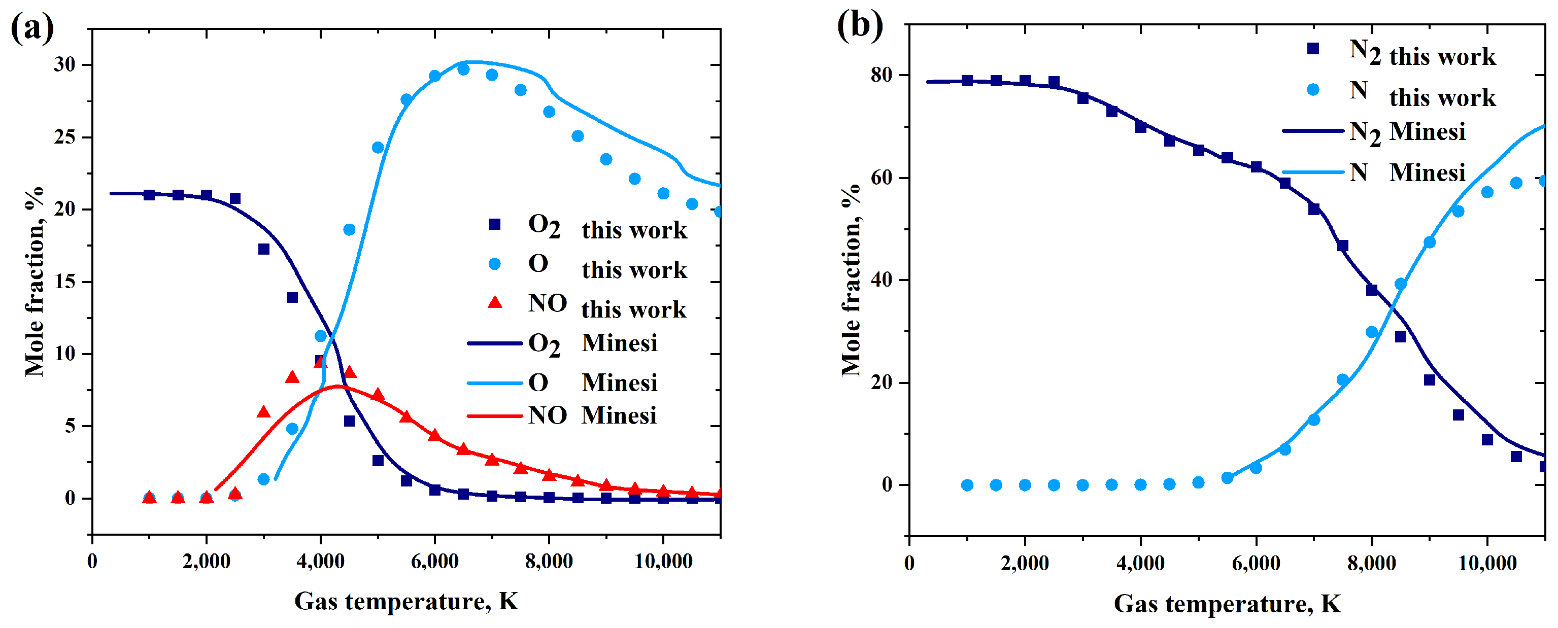
2.5.1. The Chemistry Mechanism

The composition of species in equilibrium air discharge in temperature range from 300 K to 10,000 K with constant volume process is calculated to test the chemistry mechanism. Its initial composition of the mixture is air (21% ${\mathrm{O}}_2$ and 79% ${\mathrm{N}}_2$) at the atmospheric pressure and a temperature of 300 K. Electron temperature is equal to gas temperature to calculate the equilibrium composition of air in different temperature. We compute a sufficiently long time (>1 s) to reach equilibrium state. The mole fraction of the species in the equilibrium state is shown in Figure 5. The dot is calculated using this mechanism, and the solid line is calculated by Minesi et al. [32]. The mole fraction is very close to that reported by Minesi et al. [32], which ensures the accuracy of the chemical mechanism and program code.

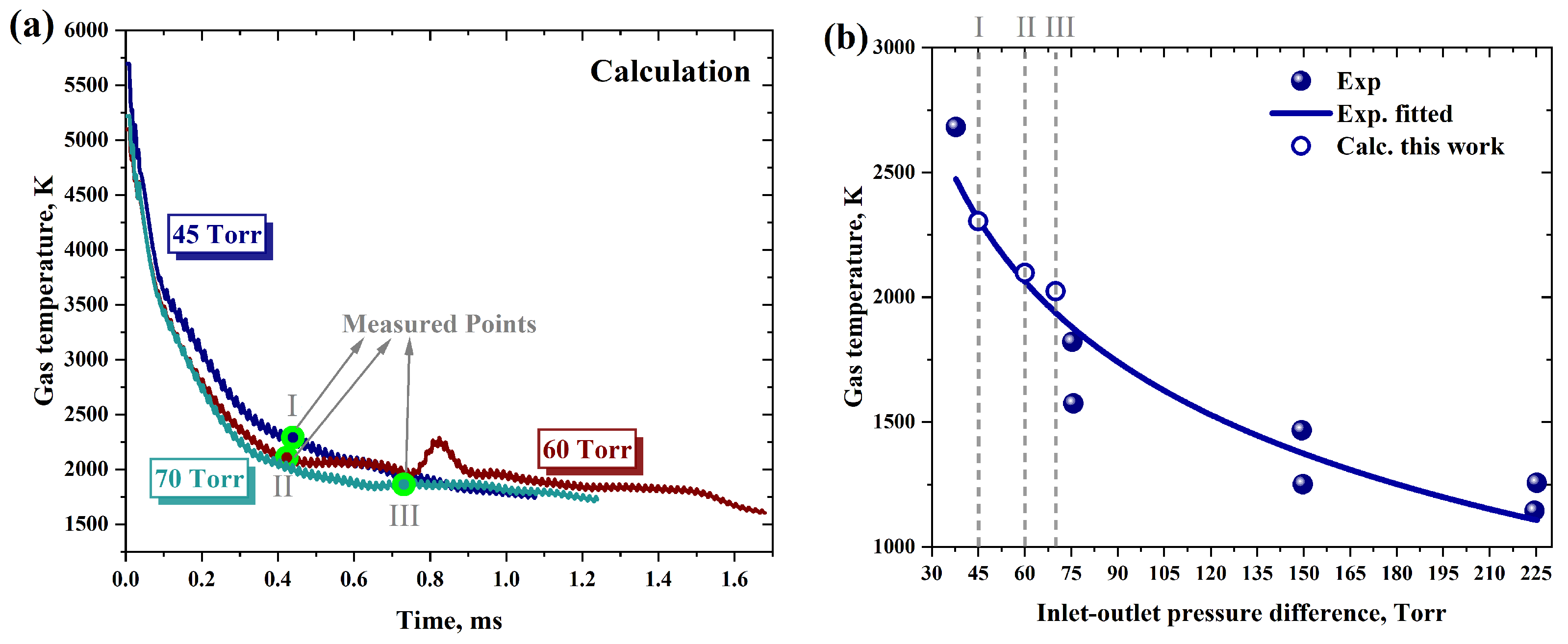
2.5.2. The Outlet Temperature

Temperature is one of the outputs of the global chemistry model and can be used for direct validation. An experimental measurement of the gliding arc temperature is conducted in similar conditions in a previous publication [34]. The temperature of the gliding arc 10 mm from the igniter exit under different inlet-outlet pressure differences is measured using a thermocouple with a measurement time no more than 20 s, as shown in Figure 6b. This temperature is a stable gliding arc temperature over a long time (several s) but not a transient temperature. The temperature of the global chemistry model is a transient temperature in specific time. We compare the transient temperature calculated using the global chemistry model with the stable temperature measured using the thermocouple. It should be noted that the authors of [35] compare the temperature of a radio frequency atmospheric plasma measured using a thermocouple and the emission spectroscopy of OH and Argon, respectively, and find that the thermocouple is accurate and suitable for plasma temperature measurement.

In order to allow the transient temperature of the model to become close to the stable one, we selected the time that the gliding arc was stably generated from the igniter. As shown in Figure 7a, there are multiple atypical and unstable re-ignitions in the middle of the gliding arc before 5 ms and typical and stable re-ignitions at the igniter exit after 5 ms. So the voltage, current and the evolution photographs of the gliding arc captured in our experiment from $6.15$ ms to $7.35$ ms with the pressure difference of 45 Torr were inputted into the global chemistry model. Partial photographs of the gliding arc are used to get the length and radius of the gliding arc shown in Figure 7b. The simulation time at other pressures is selected with the same principle of 45 Torr. The voltage and current data are provided in the Supplementary Materials. The initial conditions of the coupled 3D–0D model are shown in

Table 2. Initial conditions of the coupled 3D–0D model.

Model	Variable	Case I	Case II	Case III
The 3D gas dynamics model	Inlet gage pressure	45 Torr	60 Torr	75 Torr
	Outlet gage pressure	0 Torr	0 Torr	0 Torr
The global chemistry model	Gas temperature	5700 K	5100 K	5220 K
	Mole fraction of N2	0.79	0.79	0.79
	Mole fraction of O2	0.21	0.21	0.21
	Power	From experiment
	Air velocity	From the 3D gas dynamics model

. We use the global chemistry model to calculate the gliding arc temperature evolution at various pressure differences shown in Figure 6a. The temperature of the gliding arc 10 mm from the igniter exit is indicated by the green circle. The temperature of the gliding arc calculated using this global chemistry model is very close to the experimental one, with an error ranging from 50 K to 110 K as shown in Figure 6b.

3. Results and Discussion

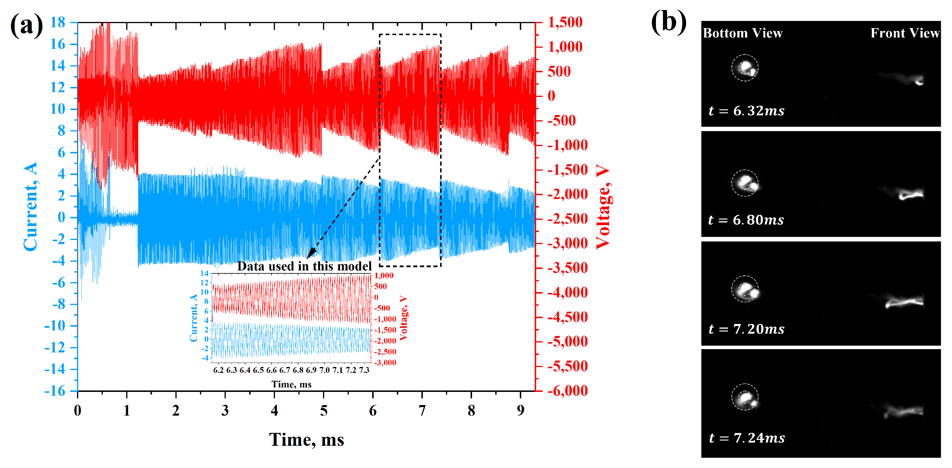
3.1. The Structure of the Flow in/out of the Gliding Arc Igniter

As shown in Figure 8, the airflow of the igniter and the lower cavity is calculated using the $k-\epsilon$ model when the pressure difference is 45 Torr. The position of the maximum velocity of over 100 m/s is near the inlet of the igniter. The maximum value of 30 m/s in the legend on the left side of the figure is artificially set to make the velocity field at the exit more obvious. The swirling flow field generated in the igniter is illustrated on the right-hand side of the figure. We use the velocity of the outlet center of the igniter as the input for the global chemistry model, which is pointed out in the figure.

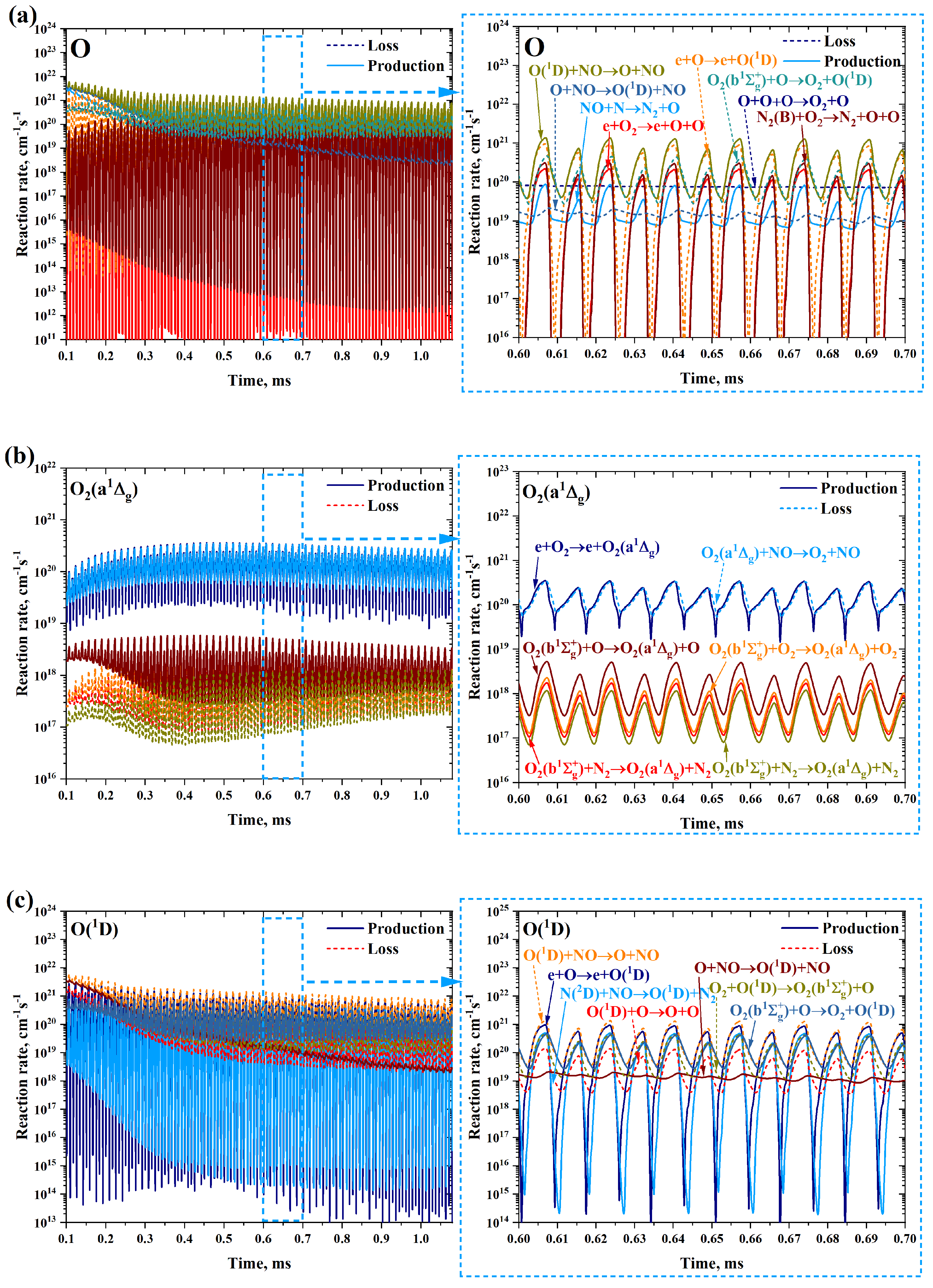
3.2. Transition from Equilibrium to Non-Equilibrium

The gas temperature and species density of the gliding arc in the situation of the inlet–outlet pressure difference reaching 45 Torr, are calculated using this global chemistry model. The gliding arc reignites close to the igniter outlet, and the gliding arc then transitions from a chemical equilibrium state to a non–equilibrium state. As shown in Figure 9a, the gliding arc temperature drops sharply from 5700 K to 4500 K during the transition. The excited species $\mathrm{O}$ and ${\mathrm{O}}_2$ are extinguished and many ground state $\mathrm{O}$ atoms were generated. The electron density decreases from ${10}^{18}$ ${\mathrm{cm}}^{-3}$ to ${10}^{14}$ ${\mathrm{cm}}^{-3}$ and the degree of ionization is reduced greatly. The distance in Figure 9a represents the distance between the head of the gliding arc and the anode at this moment captured using a high-speed camera.

A source rate analysis of the gas temperature is conducted to determine the reason for the transition from equilibrium to non–equilibrium. As shown in Figure 10a, the total heat loss fluctuates and is negative most of the time. This is mainly because the convective heat transfer loss is greater than the power heat from the power supply. Thus, the temperature of gliding arc decreases quickly from 5700 K, and the gliding arc then transitions from kinetic equilibrium to non–equilibrium. Joule heat and the effect of gliding arc growth slightly influence the gliding arc transition. It indicates that the equilibrium between convective heat transfer and power heat decide the transition moment. Since convective heat transfer actually depends on the air flow speed, this lays a theoretical foundation for the control of the transition time by controlling the air flow velocity/gliding arc ignition pressure difference between the inside and outside of the igniter, so as to realize the switching control of gliding arc heat effect (temperature) and chemical effect (active species density).

During the transition, the EEDF should be changed from the Maxwellian distribution to another. We assume that the EEDF in the transition stage follows the Maxwellian distribution and cannot capture the changes in EEDF in the transition stage. Only when the gas temperature is less than 4000 K and the electron density is less than $1.5\times {10}^{15}$ ${\mathrm{cm}}^{-3}$ can it enter the non-equilibrium stage, then the EEDF changes according to Boltzmann equation. Therefore, we compare the EEDF in the transition stage with that in the non-equilibrium stage, as shown in Figure 10b. The Maxwellian distribution has a higher EEDF value at a low electron energy level (<1.0 eV) than the EEDF in the non–equilibrium stage. However, at a higher electron energy level ($1.0$–2.5 eV), the EEDF in the non–equilibrium stage has a higher value than the Maxwellian distribution. We found that the EEDF in the non–equilibrium stage had a positive correlation with the reduced electric field. The larger the reduced electric field, the larger the EEDF at the high electron energy level (>$1.0$ eV). Owing to the power supply with alternating current, the reduced electric field and EEDF changed correspondingly.

We compare the changes of species density at times $0.1$ ms and $1.05$ ms compared to the highly ionized stage, as shown in Figure 11. The relative multiples of increase or decrease are calculated using Equation (21) or Equation (22), where $n_a$ is the species density after transition and $n_{eq}$ is the species density in the highly ionized stage. In the initial non–equilibrium stage at $0.1$ ms, we find that species density of ${\mathrm{O}}^{+}$, $\mathrm{electron}$, $\mathrm{O}{(}^1\mathrm{S})$, and ${\mathrm{O}}_2\left({\mathrm{a}}^1{\mathsf{\Delta }}_{\mathrm{g}}\right)$ decrease sharply by over two orders of magnitude, whereas species density of ${\mathrm{O}}_3$ and ${\mathrm{O}}_2$ increase dramatically by over four orders of magnitude. Compared with the period at $0.1$ ms, more ${\mathrm{O}}_3$ is generated during the non–equilibrium stage at $1.05$ ms.

$$Q_i=\frac{n_a-n_{eq}}{n_{eq}}$$

(21)

$$Q_d=\frac{n_{eq}-n_a}{n_a}$$

(22)

$\mathrm{O}$, ${\mathrm{O}}_2\left({\mathrm{a}}^1{\mathsf{\Delta }}_{\mathrm{g}}\right)$ and $\mathrm{O}{(}^1\mathrm{D})$ are the critical species for starting chemical chain. So species source rate analysis for those three species is conducted, as shown in Figure 9b–d. In transition stage, owing to high gliding arc temperature, $\mathrm{O}$ atoms achieve dynamic equilibrium through reactions (23) and (24) and the density sustains in $5\times {10}^{17}$ ${\mathrm{cm}}^{-3}$.

$$\mathrm{NO}+\mathrm{N}\leftrightarrow {\mathrm{N}}_2+\mathrm{O}$$

(23)

$$\mathrm{O}{(}^1\mathrm{D})+\mathrm{O}\leftrightarrow \mathrm{O}+\mathrm{O}$$

(24)

${\mathrm{O}}_2\left({\mathrm{a}}^1{\mathsf{\Delta }}_{\mathrm{g}}\right)$ is generated mainly through electron impact excitation reaction (25), and in transition stage, is quenched through quenching reaction (26) by collision with NO.

$$\mathrm{e}+{\mathrm{O}}_2\to \mathrm{e}+{\mathrm{O}}_2\left({\mathrm{a}}^1{\mathsf{\Delta }}_{\mathrm{g}}\right)$$

(25)

$${\mathrm{O}}_2\left({\mathrm{a}}^1{\mathsf{\Delta }}_{\mathrm{g}}\right)+\mathrm{NO}\to {\mathrm{O}}_2+\mathrm{NO}$$

(26)

In the condition of low electron temperature and high gas temperature, species density of $\mathrm{O}{(}^1\mathrm{D})$ is under relative low level and sustain in dynamic equilibrium through the reactions (27)–(29) by collision with NO, O and electron, respectively.

$$\mathrm{O}{(}^1\mathrm{D})+\mathrm{NO}\leftrightarrow \mathrm{O}+\mathrm{NO}$$

(27)

$$\mathrm{O}{(}^1\mathrm{D})+\mathrm{O}\leftrightarrow \mathrm{O}+\mathrm{O}$$

(28)

$$\mathrm{O}{(}^1\mathrm{D})+\mathrm{e}\leftrightarrow \mathrm{O}+\mathrm{e}$$

(29)

In conclusion, the transition of the gliding arc from equilibrium to non–equilibrium occur because the convective heat loss is larger than the power heat from the power supply. During the transition, many excited species extinguish and generat a large amount of $\mathrm{O}$, ${\mathrm{O}}_2$, and ${\mathrm{O}}_3$ and release considerable heat.

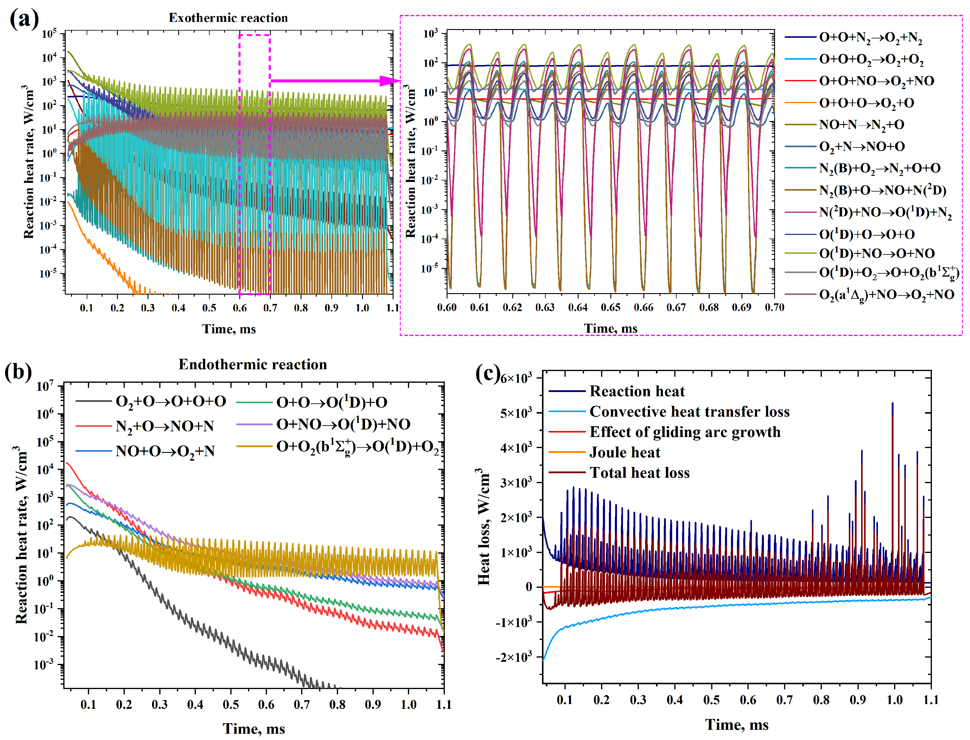
3.3. Extinction of the Non-Equilibrium Gliding Arc

According to the model calculation results shown in Figure 12, under the condition of 45 Torr pressure difference, the gliding arc will complete the equilibrium-non–equilibrium transition at about 2 mm from the exit, enter the non-equilibrium phase, and evolve to complete the non-equilibrium stage at 56 mm from the outlet, then the gliding arc will enter the extinguishment stage.

The non–equilibrium stage is marked by the A interval as shown in Figure 12, the gas temperature decreases gradually from 4500 K to 1735 K, and the electron temperature is maintained at 14,000 ± 6000 K as shown in Figure 12. Many excited species, such as $\mathrm{O}{(}^1\mathrm{S})$, $\mathrm{O}{(}^1\mathrm{D})$, ${\mathrm{O}}_2\left({\mathrm{a}}^1{\mathsf{\Delta }}_{\mathrm{g}}\right)$, and ${\mathrm{O}}_2\left({\mathrm{b}}^1{\Sigma }_{\mathrm{g}}^{+}\right)$, are produced effectively in non–equilibrium stage, owing to the high electron temperature (up to 14,000 K). As the plasma power supply is an alternating current, the reduced electric field and electron energy change accordingly. O atoms decrease slowly to ${10}^{17}$ ${\mathrm{cm}}^{-3}$. The density of $\mathrm{O}{(}^1\mathrm{D})$, ${\mathrm{O}}_2\left({\mathrm{a}}^1{\mathsf{\Delta }}_{\mathrm{g}}\right)$, ${\mathrm{O}}_2\left({\mathrm{b}}^1{\Sigma }_{\mathrm{g}}^{+}\right)$ and ${\mathrm{O}}_3$ sustain in ${10}^{13}$–${10}^{14}$ ${\mathrm{cm}}^{-3}$ with a relative high level, but the density of $\mathrm{O}{(}^1\mathrm{S})$ is lower than ${10}^{12}$ ${\mathrm{cm}}^{-3}$ and fluctuates significantly.

Compared to the transition stage, since the gliding arc spends more time in the non–equilibrium stage, the critical species O, $\mathrm{O}{(}^1\mathrm{D})$, ${\mathrm{O}}_2\left({\mathrm{a}}^1{\mathsf{\Delta }}_{\mathrm{g}}\right)$ in this stage are more important in ignition and plasma assisted combustion, so the source rate analysis of the species in the non-equilibrium stage is conducted, as shown in Figure 13. The details of the source rate analysis from $0.6$ ms to $0.7$ ms are presented on the right-hand side of the figure. In the source rate analysis of O atoms shown in Figure 13a, unlike the transition stage, which mainly maintains the balance of forward and reverse reactions through reactions (23) and (24), in the non–equilibrium gliding arc with relatively high electron temperature, O atoms are activated by electron collision excitation reaction (29) and reaction (30), and are generated through forward reaction of (27), thus maintaining the density dynamic balance between O and $\mathrm{O}{(}^1\mathrm{D})$.

$${\mathrm{O}}_2\left({\mathrm{b}}^1{\mathsf{\Sigma }}_{\mathrm{g}}^{+}\right)+\mathrm{O}\to {\mathrm{O}}_2+\mathrm{O}\left({}^1\mathrm{D}\right)$$

(30)

Similar to the transition stage, in the non–equilibrium stage, ${\mathrm{O}}_2\left({\mathrm{a}}^1{\mathsf{\Delta }}_{\mathrm{g}}\right)$ is produced primarily through the electron impact excitation reaction (25), and is quenched through the quenching reaction (26) by collision with NO. $\mathrm{O}{(}^1\mathrm{D})$ is produced primarily through electron impact excitation reaction (31) and quenching reaction (30), and is quenched through the quenching reaction (27).

$$\mathrm{e}+\mathrm{O}\to \mathrm{e}+\mathrm{O}{(}^1\mathrm{D})$$

(31)

From the source rate analysis of the gas temperature and reaction heat shown in Figure 14, the gas temperature is primarily determined by reaction heat and convective heat transfer, but joule heat and effect of gliding arc growth have little influence. Along with the decrease in gas temperature, the convective heat transfer loss becomes smaller. Reaction heat fluctuates with power supply. The total heat loss fluctuates and is negative most of the time, so the gas temperature decreases constantly. As shown in Figure 14, the source rate analysis in the exothermic reaction section indicates that the gliding arc mainly occurs through O atom compound reaction (32) and reaction (27) between $\mathrm{O}{(}^1\mathrm{D})$ and NO to release heat.

$$\mathrm{O}+\mathrm{O}+{\mathrm{N}}_2\to {\mathrm{O}}_2+{\mathrm{N}}_2$$

(32)

Source rate analysis in the exothermic reaction part indicates that, in the early non–equilibrium stage with high gas temperature, the gliding arc mainly occurs through reactions (33) and (34) to absorb heat. In the late non–equilibrium stage, gas temperature decreases to 2000–2500K, and the gliding arc is mainly through reaction (30) to absorb heat.

$${\mathrm{N}}_2+\mathrm{O}\to \mathrm{NO}+\mathrm{N}$$

(33)

$$\mathrm{O}+\mathrm{NO}\to \mathrm{O}{(}^1\mathrm{D})+\mathrm{NO}$$

(34)

With the further decrease in the gas temperature and electron temperature, the gliding arc conductivity decreases sharply, and the gliding arc finally enters the extinction stage marked by the B interval. In this stage, the gas temperature drops sharply from 1800 K to 500 K, and the number of excited species decreases significantly. This is because a new gliding arc is formed at the exit of the igniter and no energy is applied to the old gliding arc. The density of $\mathrm{O}$ decreases from ${10}^{17}$ ${\mathrm{cm}}^{-3}$ to ${10}^{16}$ ${\mathrm{cm}}^{-3}$ through reactions (32) and (35)–(37), and then generates a large number of ${\mathrm{O}}_2$. O elements exist mainly in species of O and O₂. ${\mathrm{O}}_3$ density remains unchanged with a value of ${10}^{14}$ ${\mathrm{cm}}^{-3}$.

$$\mathrm{O}+\mathrm{O}+\mathrm{NO}\to {\mathrm{O}}_2+\mathrm{NO}$$

(35)

$$\mathrm{O}+\mathrm{O}+{\mathrm{O}}_2\to {\mathrm{O}}_2+{\mathrm{O}}_2$$

(36)

$$\mathrm{O}+\mathrm{O}+\mathrm{O}\to {\mathrm{O}}_2+\mathrm{O}$$

(37)

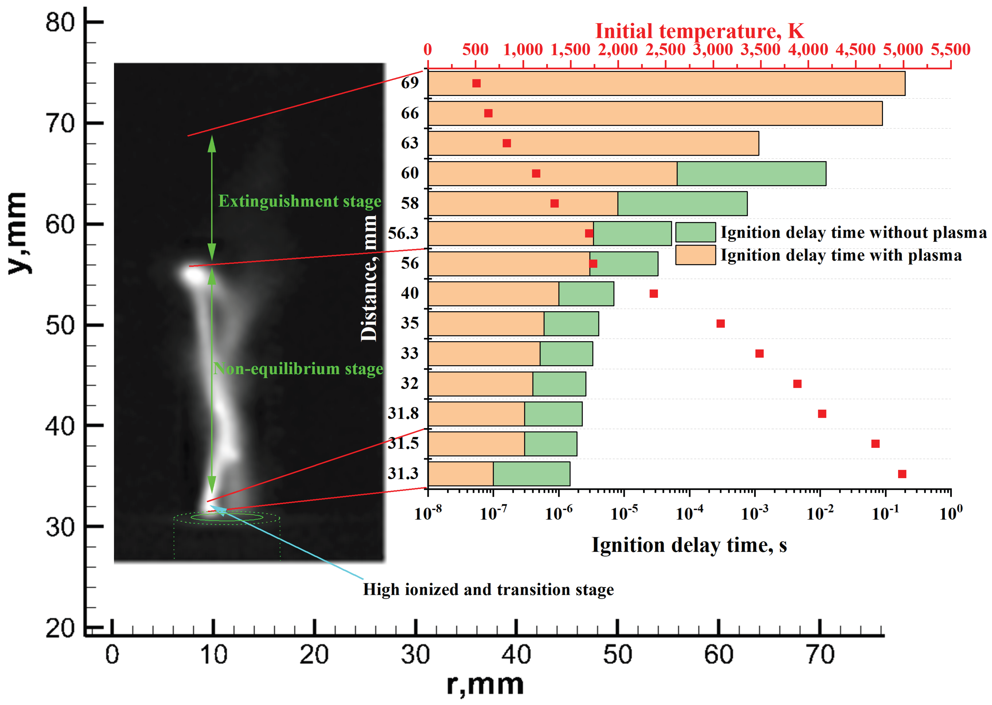
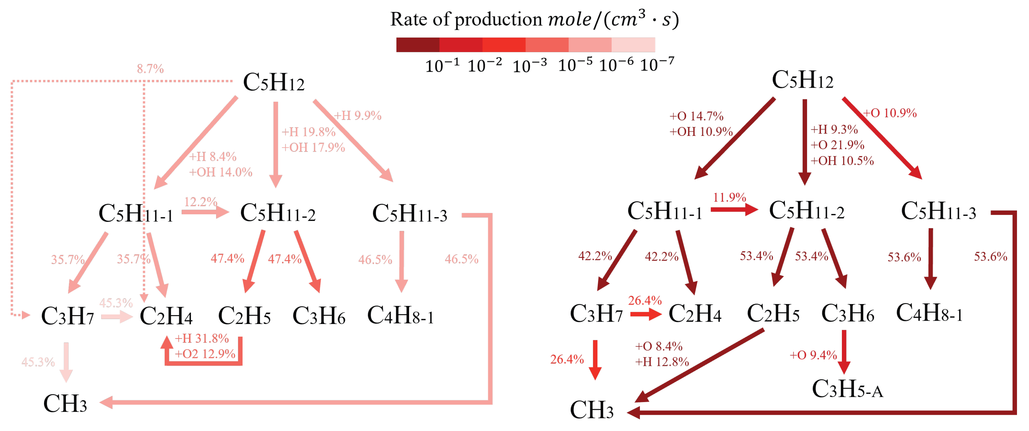
3.4. A Test Case of Gliding Arc-Assisted Ignition

To analyze the influence of the different stages on pentane combustion, we extract the density and temperature of the species at different positions that the head of the gliding arc reach. We use the mechanism [36] to study gliding arc–assisted pentane combustion, which has been validated with experiment. The species density and gas temperature are obtained from Chemkin to calculate the ignition delay time. The ignition delay time is calculated under the assumption that the plasma species at any position of the gliding arc are fully premixed with the fuel. The ignition delay time with the plasma consider the excited species and atoms produced by the gliding arc. The ignition delay time without plasma does not consider the excited species and atoms but considers the influence of gas temperature on pentane combustion.

As shown in Figure 15, the initial temperature decreases with the increase in distance, and the ignition delay time increases with the increasing in distance. In the non–equilibrium stage, the ignition delay time with plasma ranges from $4.0\times {10}^{-7}$ s to $3.0\times {10}^{-6}$ s whereas that without plasma ranges from $2.6\times {10}^{-6}$ s to $3.3\times {10}^{-5}$ s. Overall, the ignition delay time with plasma was reduced by 82–90% compared to the ignition delay time without plasma.

In the extinguishment stage, pentane combustion without plasma can successfully ignite before 60 mm, whereas that with plasma can successfully ignite before 69 mm. This indicates that the plasma can shorten the fuel ignition temperature and that the effective arc penetration lengths of 30 and 40 mm are determined based on the thermal and chemical effects of plasma, respectively. At 60 mm, the ignition delay time with plasma is 0.5% of that without plasma. This suggests that the chemical effect plays a significant role in pentane combustion at 1100 K.

We analyze the reaction path of pentane combustion with and without plasma at 60 mm. As shown in Figure 16, the overall rate of production of combustion with plasma is four orders of magnitude higher than that of combustion without plasma. The consumption pathway does not show any significant changes.

We compare the species density and gas temperature when pentane conversion is 50%, as shown in Figure 17. The gas temperature with plasma is 100 K higher than that without plasma, which demonstrates that plasma exerts a thermal effect to enhance combustion. The mole fractions of H, O, and OH with plasma are far larger than those without plasma because the gliding arc produces many O atoms. The O atoms can accelerate pentane splitting through H abstraction to produce ${\mathrm{C}}_5{\mathrm{H}}_{11}$ and $\mathrm{OH}$. Subsequently, ${\mathrm{C}}_5{\mathrm{H}}_{11}$ can be split into small molecules (${\mathrm{C}}_2{\mathrm{H}}_5$, ${\mathrm{C}}_3{\mathrm{H}}_6$…). These small molecules can react with O to produce H and RCHO. Thus, pentane combustion with plasma generates more H, O, and $\mathrm{OH}$ atoms, which accelerates pentane splitting. This demonstrates that plasma exerts a chemical effect to enhance combustion.

4. Conclusions

A self–consistent model, coupling the global chemistry model, the 3D gas dynamics model, and experimental data, is developed to obtain a deeper insight into the performance and mechanism of gliding arc–based plasma devices. This model just considers the experimental power supply and the length and structure of the gliding arc device as inputs and can output the gliding arc species density and temperature. Moreover, the model has been validated with the experimental gliding arc temperature [34]. With less computation cost and easy–to–obtain experimental data, the model can not only quickly predict the species density and temperature of the gliding arc in an igniter, but also can be applied to more general gliding arc devices (e.g., an arc touch for nitrogen fixation).

During the transition, the gas temperature decreases sharply from 5700 K to 4500 K. The energy deposited by the power source cannot compensate for the convective heat transfer loss, causing the decrease in gas temperature and the occurrence of gliding arc transition. Joule heat and effect of gliding arc growth take a little influence on gliding arc transition, and the equilibrium between convective heat transfer and power heat decide the transition. Owing to high gliding arc temperature, $\mathrm{O}$ atoms achieve dynamic equilibrium through reactions (23) and (24) and the density sustains in $5\times {10}^{17}$ ${\mathrm{cm}}^{-3}$. ${\mathrm{O}}_2\left({\mathrm{a}}^1{\mathsf{\Delta }}_{\mathrm{g}}\right)$ is quenched through quenching reaction (26) by collision with NO. Species density of $\mathrm{O}{(}^1\mathrm{D})$ is under relative low level and sustain in dynamic equilibrium through the reactions (27)–(29) by collision with NO, O and electron, respectively.

In non–equilibrium stage, the gas temperature decreases gradually from 4500 K to 1735 K, and the electron temperature is maintained at 14,000 ± 6000 K. The gas temperature is primarily determined by reaction heat and convective heat transfer, but joule heat and effect of gliding arc growth have little influence. Source rate analysis indicates that the gliding arc is mainly through O atom compound reaction (32) and reaction (27) between $\mathrm{O}{(}^1\mathrm{D})$ and NO to release heat. O atoms are activated by electron collision excitation reaction (29) and reaction (30), and are generated through forward reaction of (27), thus maintaining the density dynamic balance between O and $\mathrm{O}{(}^1\mathrm{D})$. Similar to the transition stage, ${\mathrm{O}}_2\left({\mathrm{a}}^1{\mathsf{\Delta }}_{\mathrm{g}}\right)$ is produced primarily through the electron impact excitation reaction (25), and is quenched through the quenching reaction (26) by collision with NO. $\mathrm{O}{(}^1\mathrm{D})$ is produced primarily through electron impact excitation reaction (31) and quenching reaction (30), and is quenched through the quenching reaction (27) with NO.

Effective arc penetration lengths of 30 mm and 40 mm are determined based on the thermal and chemical effects of the gliding arc, respectively. In the non–equilibrium stage, the ignition delay time with plasma was reduced by 82–90% compared to the ignition delay time without plasma. The overall rate of production of combustion with plasma is four orders of magnitude larger than that of combustion without plasma. O atoms produced in the gliding arc can accelerate the pentane and fuel fragment splitting to generate H and $\mathrm{OH}$ atoms, then those atoms further accelerate fuel fragment splitting, which demonstrates the chemical effect of the gliding arc.

References

1. Ju, Y.; Lefkowitz, J.K.; Reuter, C.B.; Won, S.H.; Yang, X.; Yang, S.; Sun, W.; Jiang, Z.; Chen, Q. Plasma assisted low temperature combustion. Plasma Chem. Plasma Process. 2016, 36, 85–105. [Google Scholar] [CrossRef] [Green Version]
2. Fridman, A. Plasma Chemistry; Cambridge University Press: Cambridge, UK, 2008. [Google Scholar]
3. Foster, J.E. Plasma-based water purification: Challenges and prospects for the future. Phys. Plasmas 2017, 24, 055501. [Google Scholar] [CrossRef]
4. Barjasteh, A.; Dehghani, Z.; Lamichhane, P.; Kaushik, N.; Choi, E.H.; Kaushik, N.K. Recent progress in applications of non-thermal plasma for water purification, bio-sterilization, and decontamination. Appl. Sci. 2021, 11, 3372. [Google Scholar] [CrossRef]
5. Hong, S.H.; Kim, T.H.; Choi, S. Hydrophilic surface modification of polytetrafluoroethylene film with gliding arc plasma. Appl. Sci. Converg. Technol. 2019, 28, 101–106. [Google Scholar] [CrossRef]
6. Macedo, M.J.; Silva, G.S.; Feitor, M.C.; Costa, T.H.; Ito, E.N.; Melo, J.D. Surface modification of kapok fibers by cold plasma surface treatment. J. Mater. Res. Technol. 2020, 9, 2467–2476. [Google Scholar] [CrossRef]
7. Wang, W.; Berthelot, A.; Kolev, S.; Tu, X.; Bogaerts, A. CO2 conversion in a gliding arc plasma: 1D cylindrical discharge model. Plasma Sources Sci. Technol. 2016, 25, 065012. [Google Scholar] [CrossRef]
8. Trenchev, G.; Kolev, S.; Wang, W.; Ramakers, M.; Bogaerts, A. CO2 conversion in a gliding arc plasmatron: Multidimensional modeling for improved efficiency. J. Phys. Chem. C 2017, 121, 24470–24479. [Google Scholar] [CrossRef]
9. Van Alphen, S.; Slaets, J.; Ceulemans, S.; Aghaei, M.; Snyders, R.; Bogaerts, A. Effect of N2 on CO2-CH4 conversion in a gliding arc plasmatron: Can this major component in industrial emissions improve the energy efficiency? J. CO2 Util. 2021, 54, 101767. [Google Scholar] [CrossRef]
10. Li, L.; Zhang, H.; Li, X.; Kong, X.; Xu, R.; Tay, K.; Tu, X. Plasma-assisted CO2 conversion in a gliding arc discharge: Improving performance by optimizing the reactor design. J. CO2 Util. 2019, 29, 296–303. [Google Scholar] [CrossRef]
11. Song, F.; Wu, Y.; Yang, X.K.; Zhou, J.P.; Chen, X. Gliding arc plasma adjusting pre-combustion cracking products. Def. Technol. 2022, 18, 2198–2202. [Google Scholar] [CrossRef]
12. Lin, B.; Wu, Y.; Zhu, Y.; Song, F.; Bian, D. Experimental investigation of gliding arc plasma fuel injector for ignition and extinction performance improvement. Appl. Energy 2019, 235, 1017–1026. [Google Scholar] [CrossRef]
13. Huang, S.; Wu, Y.; Zhang, K.; Jin, D.; Zhang, Z.; Li, Y. Experimental investigation of spray characteristics of gliding arc plasma airblast fuel injector. Fuel 2021, 293, 120382. [Google Scholar] [CrossRef]
14. Kai, Z.; Feilong, S.; Di, J.; Shida, X.; Jiulun, S.; Shengfang, H. Experimental investigation on the cracking of pre-combustion cracking gas with gliding arc discharge plasma. Int. J. Hydrogen Energy 2021, 46, 9019–9029. [Google Scholar] [CrossRef]
15. Wang, W.Z.; Jia, M.; Feng, R.; Zhu, J.J. Experimental investigation on the gliding arc plasma supported combustion in the scramjet combustor. Acta Astronaut. 2020, 177, 133–141. [Google Scholar] [CrossRef]
16. Liming, H.; Yi, C.; Jun, D.; Jianping, L.; Li, F.; Pengfei, L. Experimental study of rotating gliding arc discharge plasma-assisted combustion in an aero-engine combustion chamber. Chin. J. Aeronaut. 2019, 32, 337–346. [Google Scholar]
17. Feng, R.; Huang, Y.; Zhu, J.; Wang, Z.; Sun, M.; Wang, H.; Cai, Z. Ignition and combustion enhancement in a cavity-based supersonic combustor by a multi-channel gliding arc plasma. Exp. Therm. Fluid Sci. 2021, 120, 110248. [Google Scholar] [CrossRef]
18. Feng, R.; Li, J.; Wu, Y.; Jia, M.; Jin, D. Ignition and blow-off process assisted by the rotating gliding arc plasma in a swirl combustor. Aerosp. Sci. Technol. 2020, 99, 105752. [Google Scholar] [CrossRef]
19. Wu, W.W.; Ni, G.H.; Lin, Q.F.; Guo, Q.J.; Meng, Y.D. Experimental investigation of premixed methane–air combustion assisted by alternating-current rotating gliding arc. IEEE Trans. Plasma Sci. 2015, 43, 3979–3985. [Google Scholar] [CrossRef]
20. Ombrello, T.; Ju, Y.; Fridman, A. Kinetic ignition enhancement of diffusion flames by nonequilibrium magnetic gliding arc plasma. AIAA J. 2008, 46, 2424–2433. [Google Scholar] [CrossRef]
21. Pinto, A.; Sbampato, M.; Sagás, J.; Lacava, P. Gliding arc discharge for emission control in swirl fuel-lean non-premixed combustion. Combust. Sci. Technol. 2021, 195, 1235–1250. [Google Scholar] [CrossRef]
22. Pellerin, S.; Richard, F.; Chapelle, J.; Cormier, J.; Musiol, K. Heat string model of bi-dimensional dc Glidarc. J. Phys. D Appl. Phys. 2000, 33, 2407. [Google Scholar] [CrossRef]
23. Richard, F.; Cormier, J.; Pellerin, S.; Chapelle, J. Physical study of a gliding arc discharge. J. Appl. Phys. 1996, 79, 2245–2250. [Google Scholar] [CrossRef]
24. Kolev, S.; Bogaerts, A. A 2D model for a gliding arc discharge. Plasma Sources Sci. Technol. 2014, 24, 015025. [Google Scholar] [CrossRef]
25. Sun, S.; Kolev, S.; Wang, H.; Bogaerts, A. Coupled gas flow-plasma model for a gliding arc: Investigations of the back-breakdown phenomenon and its effect on the gliding arc characteristics. Plasma Sources Sci. Technol. 2016, 26, 015003. [Google Scholar] [CrossRef]
26. Wang, W.; Mei, D.; Tu, X.; Bogaerts, A. Gliding arc plasma for CO2 conversion: Better insights by a combined experimental and modelling approach. Chem. Eng. J. 2017, 330, 11–25. [Google Scholar] [CrossRef]
27. Bourlet, A.; Labaune, J.; Tholin, F.; Vincent, A.; Pechereau, F.; Laux, C.O.; Vincent-Randonnier, A.; Laux, C.O.; Vincent, A.; Pechereau, F.; et al. Numerical model of restrikes in DC gliding arc discharges. In Proceedings of the AIAA SCITECH 2022 Forum, Virtual, 3–7 January 2022; American Institute of Aeronautics and Astronautics: Reston, VA, USA, 2022; pp. 1–10. [Google Scholar] [CrossRef]
28. Cheng, X.; Song, H.; Huang, S.; Zhu, Y.; Zhang, Z.; Li, Z.; Jia, M. Discharge and jet characteristics of gliding arc plasma igniter driven by pressure difference. Plasma Sci. Technol. 2022, 24, 115502. [Google Scholar] [CrossRef]
29. Available online: http://www.comsol.com (accessed on 5 January 2022).
30. Pancheshnyi, S.; Eismann, B.; Hagelaar, G.J.M.; Pitchford, L.C. Computer Code ZDPlasKin; University of Toulouse, LAPLACE, CNRS-UPS-INP: Toulouse, France, 2008; Available online: http://www.zdplaskin.laplace.univ-tlse.fr (accessed on 5 April 2022).
31. Hagelaar, G.; Pitchford, L.C. Solving the Boltzmann equation to obtain electron transport coefficients and rate coefficients for fluid models. Plasma Sources Sci. Technol. 2005, 14, 722. [Google Scholar] [CrossRef]
32. Minesi, N. Thermal Spark Formation and Plasma-Assisted Combustion by Nanosecond Repetitive Discharges. Ph.D. Thesis, Université Paris-Saclay, Gif-sur-Yvette, France, 2020. [Google Scholar]
33. Rong, M. Gas Discharge Plasma Database. Available online: http://www.plasma-data.net/index (accessed on 5 April 2022).
34. Mikhailov, V.; Lebedev, V.; Mukhin, A. Experimental development of a plasma spark plug for GTE altitude start. Russ. Aeronaut. (Iz VUZ) 2010, 53, 235–241. [Google Scholar] [CrossRef]
35. Doyle, S.; Xu, K. Use of thermocouples and argon line broadening for gas temperature measurement in a radio frequency atmospheric microplasma jet. Rev. Sci. Instrum. 2017, 88, 023114. [Google Scholar] [CrossRef] [Green Version]
36. Rousso, A.; Mao, X.; Chen, Q.; Ju, Y. Kinetic studies and mechanism development of plasma assisted pentane combustion. Proc. Combust. Inst. 2019, 37, 5595–5603. [Google Scholar] [CrossRef]
Figure 1. Characteristics of the gliding arc experiment system.
Processes 11 00873 g001
Figure 2. (a) The twin-duct ignition platform and (b) the schematic diagram of the gliding arc igniter structure.
Processes 11 00873 g002
Figure 3. Computational domain of the 3D gas dynamics model. The inlet, outlet, cathode and anode are indicated. (a) The front view and (b) the section view.
Processes 11 00873 g003
Figure 4. Combined schematic of the experimental system and the global chemistry model.
Processes 11 00873 g004
Figure 5. Equilibrium composition of the synthetic air as a function of the temperature in a constant volume process. (a) Comparison of O 2 , O , NO mole fractions, (b) Comparison of N 2 and N mole fractions.
Processes 11 00873 g005
Figure 6. (a) The evolution of the calculated gliding arc temperature at various inlet-outlet pressure differences. The gliding arc temperature 10 ms from the outlet is indicated by the green cycles. The time 0 ms correspond to the re-ignition moment. (b) Comparison of the gliding arc temperature between the measurement [34] and simulation.
Processes 11 00873 g006
Figure 7. The voltage–current profile (a) measured by an oscilloscope and the evolution photographs of the gliding arc (b) captured by a high–speed camera in our experiment with the pressure difference of 45 Torr.
Processes 11 00873 g007
Figure 8. Air velocity of the igniter and the lower cavity with a pressure difference of 45 Torr. The slice view of the igniter is shown on the left and the streamline diagram is shown on the right.
Processes 11 00873 g008
Figure 9. Evolution of (a) gas temperature and species density, and (b) O , (c) O 2 a 1 Δ g , and (d) O ( 1 D ) density sensitivity analysis. The distance in photograph (a) represents the distance between the head of the gliding arc and the anode at this moment captured by a high–speed camera.
Processes 11 00873 g009
Figure 10. (a) Source rate analysis of the gas temperature and (b) the changes of EEDF during the transition.
Processes 11 00873 g010
Figure 11. The changes in species density at times (a) 0.1 ms and (b) 1.05 ms compared with the highly ionized stage.
Processes 11 00873 g011
Figure 12. The density evolution of plasma species contaning the oxygen element in the non–equilibrium and extinguishment stages. The structure schematic of the gliding arc is shown in the figure. The distance represents the distance between the head of the gliding arc and the anode at this moment captured using a high-speed camera. (A), Non–equilibrium stage, (B) Extinguishment stage.
Processes 11 00873 g012
Figure 13. Source rate analysis of species (a) O, (b) O2 (b1Δg), and (c) O(1D) in the non–equilibrium stage.
Processes 11 00873 g013
Figure 14. Source rate analysis of (a,b) reaction heat and (c) the gas temperature in the non–equilibrium stage.
Processes 11 00873 g014
Figure 15. Pentane ignition delay time of the gliding arc in different positions.
Processes 11 00873 g015
Figure 16. Fuel consumption and subsequent pathways based on the rate of production analysis when the conversion of pentane is 50%. The left photograph represents combustion without plasma, and the right photograph represents combustion with plasma.
Processes 11 00873 g016
Figure 17. Species density and temperature comparison between combustion with plasma and that without plasma when pentane conversion is 50%.
Processes 11 00873 g017