Abstract
A material balance equation (MBE) is usually employed to estimate well-controlled dynamic reserves, but a more accurate calculation of these reserves is crucial. For abnormally pressured reservoirs with aquifers, the abnormally pressure and aquifer are difficult to determine, which leads to inaccurate calculations of well-controlled dynamic reserves. In this work, the MBE was established. Then, the correction function and abnormally pressure effect were deduced to determine well-controlled dynamic reserves calculations for weak aquifers and strong aquifers, respectively. For a weak aquifer, a pressure correction was determined to exist at a pressure coefficient of 1.2, and then the correction function was established to calculate the dynamic reserves. For a strong aquifer, the MBE derived by Walsh was employed to calculate the dynamic reserves and water influx. The relationship between the abnormally pressure effect and the dimensionless formation pressure was proposed. Classical, abnormally high-pressured gas reservoirs, Anderson L and Amu Darya, were selected to validate the accuracy and applicability of the newly developed methods. The results show that an abnormally high-pressure effect has a great influence on the dynamic reserves calculation in the early stage and the water influx has a stronger influence on the dynamic reserves calculation in the late stage.
1. Introduction
Due to the effect of abnormally high pressure with bottom water influx, the relationship between p/Z and cumulative gas production volume is no longer a straight line as shown in normally pressured reservoirs, which renders the calculation of dynamic reserves difficult [1,2,3,4]. The MBE (material balance equation) has been indicated to be one of the most accurate calculation methods for well-controlled dynamic reserves of different types of gas reservoirs, whose basic principle is the conservation of matter [5,6,7]. Many material balance equations (MBEs) with different forms have been proposed by researchers to calculate the dynamic reserves involved with abnormally high-pressured or water influx issues [8,9,10,11,12].
Regarding abnormally high-pressure effects, Ramagost and Farshad (1981) considered the relationship between p/Z and cumulative gas production volume in the abnormally high-pressured phase to be a straight line. However, with a decrease in the extraction of gas and the formation pressure, the elastic expansion of gas and rock particles and the recompaction of reservoir rock are inevitable, which can supplement gas reservoir energy and reduce the formation pressure decline rate. Thus, the first straight line with a lower pressure decline is formed. As production continues downward to the normally pressured, a second straight line with a higher slope is formed. To solve the complex problem of calculation, certain scholars have proposed the form of a binomial, such as Chen and Hu (1993) [13] who proposed a dynamic reserves calculation equation in binomial form for constant volume, abnormally high-pressured reservoirs. Gonzales et al. (2008) [14] developed a binomial MBE for abnormally high-pressured reservoirs without aquifers in phases of cumulative gas production. An MBE for water-driven gas reservoirs considering the overall compressibility of rocks was established by Li (2008) [15]. The compressibility factor is expressed as a function of production characteristics, such as declining rate and gas productivity index, so only known production data are required for reserves calculation [16]. Based on the MBE of abnormally high-pressured reservoirs, a new MBE containing the squared phase of cumulative production is proposed, the parameters of which can be determined by applying production history data using binary regression analysis [17]. A new binomial MBE for predicting well-controlled dynamic reserves of gas reservoirs is proposed, exploiting the similarity between the curve shape of Ph-GpD and the IPR in abnormally high-pressured reservoirs [18]. Jiao et al. (2017) [19] proposed a new concept to describe the energy of elastic rock and water influx using the linear relationship of cumulative production, which simplifies the MBE and converts it to a multivariate nonlinear equation.
The effective compressibility of abnormally high-pressured reservoirs is related to the effective pore compressibility of rock and the compressibility and saturation of formation irreducible water, and it is difficult to accurately obtain these parameters. To solve these problems, Ramagost and Farshad (1981) [20] considered the influence of fluid and pore space to estimate the compressibility of formation rock (Cf) and immobile water (Cw); then, the effective compressibility factor of formation was determined. Pletcher (1981) [21] reorganized the MBE of a geo-pressured gas reservoir proposed by Ramagost and Farshad (1981) and derived a different linear expression, by which the original gas in place (OGIP) and the effective elastic driving force of rock or water can be simultaneously estimated. Fetkovich et al. (1998) [22] established a more complete MBE formula that can be applied to any type of reservoir. Yale et al. (1993) [23] established compressibility factor plates for unconsolidated cores, brittle cores, and strongly consolidated cores by core experiments. The empirical formula for calculating rock compressibility was established in abnormally high-pressured gas reservoirs [24]. Rahman et al. (2006) [25] proposed a rigorous MBE for geo-pressured hydrocarbon reservoirs using the origin expressions of compressibility of pore, water, and oil. The compressibility factor is no longer considered a constant but a function of pressure. A high-pressure experimental system was designed by the authors of [26], and a series of high-pressure compressibility factor tests of pure water, nitrogen, and rocks under different water saturations were carried out.
With the production of natural gas, the formation pressure declines and diffuses to the external natural waters via elastic expansion, which causes the elastic expansion of formation water and renders the calculation of dynamic reserves difficult. Therefore, to accurately calculate the water influx, certain scholars have proposed different forms of calculation methods [27]. For example, Liao (1990) [28] employed the unary, Lagrangian, three-point interpolation method and least squares curve to regress the dimensionless, natural water influx calculation formula of hemispherical flow, planar radial flow, and linear flow, thus greatly improving the calculation speed and accuracy of water influx. Fetkovich et al. (1998) [22] introduced a cumulative compressibility including pore compressibility, water compressibility, gas solubility, and any limited aquifer influx into the BME. Yang et al. (2008) [29] discussed the dynamic reserves of well control based on numerical simulation and verified the effect of the aquifer ratio on the dynamic reserves of water-driven gas reservoirs. Based on the principle of the material balance of water-driven gas reservoirs, a mathematical model of material balance was established, a new aquifer ratio parameter was introduced, and the relationship between the cumulative production of gas and that of water was obtained under well-controlled dynamic reserves and aquifer ratios that are unknown [30,31].
In this work, to solve the problems of abnormally high-pressure effects and water influx, the MBEs of abnormally high-pressured gas reservoirs with different aquifer size ratios are derived. For a weak aquifer ratio, by determining the inflection point of the curve of an abnormally high-pressure effect, a new calculation of well-controlled dynamic reserves has been established. With different aquifer size ratios, the total elastic expansion factor of the reservoir is accurately obtained by regression fitting the relationship between the dimensionless formation pressure (ppD) and the abnormally pressure effect (ĈeΔp). Next, the binomial equation for calculating well-controlled dynamic reserves and water influx is obtained. The accuracy of these methods is verified using the Anderson L gas reservoir, and the applicability and convenience of these methods are verified using the Amu Darya gas reservoir as an example.
2. Materials and Methods
2.1. MBE of Abnormally High-Pressured Reservoirs
The energy during the exploitation of reservoirs is mainly derived from the elastic expansion of natural gas, compaction of the reservoir and elastic expansion of rock particles, elastic expansion of formation immobile water, and the influx of an external aquifer. The MBE of the reservoir can be obtained by describing the above process in mathematical language:
where G is the initial dynamic reserves of the reservoir under standard conditions, 108 m3; Gp is cumulative gas production under standard conditions, 108 m3; Bgi is the volume factor of natural gas in the initial state, m3/m3; Vgi is the total pore volume of a gas field in the initial state, 108 m3; Swi is irreducible water saturation, dimensionless; Cf and Cw are the elastic factor of formation rock and water, MPa−1; Δp is formation pressure decline, MPa; We is cumulative natural water influx, m3; Wp is the cumulative water yield, m3; and Bw is the water volume factor of formation, m3/m3.
Considering Δp = pi − p and Vgi = GBgi/(1 − Swi), rearranging Equation (1) yields:
Define the formation effective compressibility factor Ce and water influx volume factor ω:
According to the expression of the natural gas volume factor:
where Z and Zi represent the natural gas deviation factor under the current reservoir conditions and original reservoir conditions, respectively, dimensionless.
Introducing Equation (2) to Equation (6) into Equation (1) and organizing it yields:
As shown in Equation (7), the difference between the pressure decline formula of abnormally high-pressured reservoirs and that of constant-volume gas reservoirs is that the former takes into account the impact of the abnormally high-pressure effect CeΔp and water influx of reservoir ω. Therefore, the determination of the above two parameters is critical to the well-controlled dynamic reserves estimation of reservoirs by the pressure decline method.
In this work, the aquifer size ratio, which is defined as the ratio of the volume of aquifer to the total gas in place at the reservoir condition, was introduced to depict the strength of aquifer energy. Herein, an aquifer ratio Mwg below 5 is classified as a weak aquifer, while a strong aquifer is classified as an aquifer ratio above 5 (Mwg ≥ 5).
2.2. Calculation of Dynamic Reserves with a Weak Aquifer Ratio
When the reservoirs have a weak aquifer, the calculation method of the Chatas water influx is approximately valid:
where raq is the outer edge radius of natural water, m.
Herein:
where Vaq is the pore volume in natural waters, m3.
The abnormally high-pressure stage is generally in the middle and early stages of development. For weak aquifers, most reservoirs still do not produce formation water (Wp = 0). Herein, introducing Equation (9) into Equation (7) yields:
where is deemed the effective compressibility factor of an abnormally high-pressured reservoir, MPa−1.
Therefore, the parameters of the abnormally high-pressure effect and aquifer size ratio can be combined, and Equation (10) has the same form as the pressure decline equation of the reservoir.
2.2.1. Establishment of the Reserves Estimation Equation
The pressure decline curve of an abnormally high–pressured, confined gas reservoir can be simplified into two straight sections, as shown in Figure 1. Section I and section II represent the two stages of abnormally high-pressured and normal pressure, respectively, in the development process, and the inflection point of the two straight lines is recorded as C.
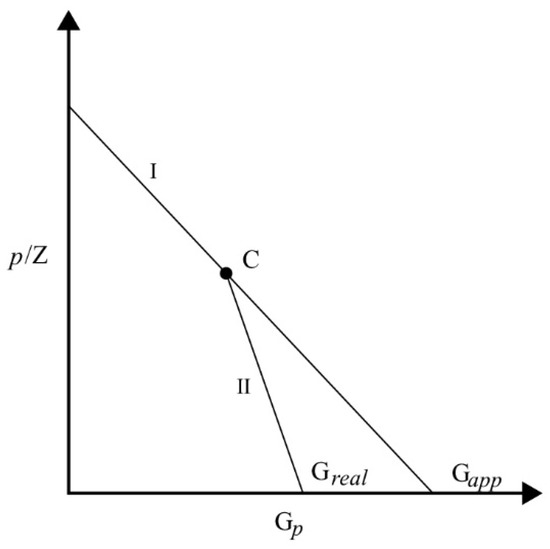
Figure 1.
The relationship between p/Z and cumulative gas production volume of the abnormally high-pressured reservoirs.
According to the MBE, describing straight-line Section I yields:
where pC is the formation pressure corresponding to the inflection point, MPa; Zc is the gas deviation factor under the condition of the inflection point, dimensionless; Gpc is the cumulative gas recovery corresponding to the formation pressure at the inflection point, 108 m3; and Gpes is the virtual dynamic reserves of the reservoir, 108 m3.
The pressure decline equation of the reservoir can be written as:
where Greal is the real dynamic reserves of the reservoir, 108 m3.
The reserves correction equation of abnormally high-pressured gas reservoirs can be obtained by combining Equations (11) and (12). When calculating well-controlled dynamic reserves of the reservoir, it is only necessary to determine the virtual dynamic reserves using the data of linear section Ⅰ and then combine it with Equation (13) to obtain the real reserves:
2.2.2. Determination of Inflection Point Position
The relationship between the abnormally pressure effect and the pressure coefficient is obtained by rearranging the pressure decline formula of the reservoir:
In order to analyze the variation rule of the abnormal high-pressure effect ĈeΔp, five typical abnormally high-pressured gas reservoirs N. Ossun, Louis. Offshore, Stafford, GOM, and Miocene S. Louis were taken as examples (Table 1). ĈeΔp values at different pressure stages were calculated according to Equation (14). The relationship between ĈeΔp and pressure coefficient (α) was analyzed to determine the variation rule of abnormally high-pressure effect (Figure 2). The pressure coefficient (α) is defined in Equation (15). The historical production data of the five typical abnormally high-pressured gas reservoirs is shown in Appendix A.
where C is the hydrostatic pressure gradient, MPa/m; D is the central depth of reservoirs, m.

Table 1.
Initial production data of the five typical abnormally high-pressured gas reservoirs.
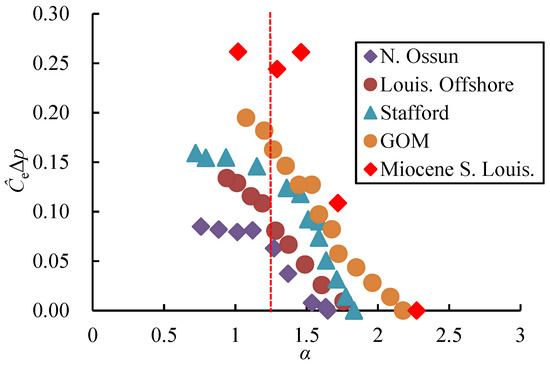
Figure 2.
Relationship between the abnormally high-pressure effect and the pressure coefficient.
The relationship between ĈeΔp and α shows two different regular patterns in Figure 2: when the pressure coefficient was greater than 1.2, ĈeΔp significantly changed with α and showed a good linear negative correlation (refer to Table 2 for the regression results); when the pressure coefficient was less than 1.2, the change in ĈeΔp with α was slow. It can be seen that α = 1.2 should be taken as the cutoff point (position of inflection point C) between the abnormally high-pressured stage and the normal pressure stage in the pressure decline diagram. The gas reservoirs mentioned in this paper all had pressure coefficients greater than 1.2, so they are all exceptionally high-pressured reservoirs.
Table 2.
Gas reservoir relational regression equation of ĈeΔp and α (α ≥ 1.2).
After determining the position of the inflection point α = 1.2 by replacing the pressure coefficient and deviation coefficient of inflection point C in Equation (13) (recorded as P1.2 and Z1.2, respectively), a new reserve estimation formula of the pressure decline method for abnormally high-pressured reservoirs can be obtained as Equation (16):
where Greal is the real dynamic reserves corresponding to the inflection point α = 1.2, 108 m3.
2.3. Calculation of Dynamic Reserves with a Strong Aquifer Ratio
In this paper, the early stage of gas reservoir development is defined as the point when the recovery degree of reservoirs is less than 10%, and the late stage is defined as the point when the recovery degree of reservoirs is more than 50%. When reservoirs have a strong aquifer (Mwg > 5), the water influx process of reservoirs cannot be simplified according to the previously described method. Herein, the MBE will have the phases of the abnormally high-pressure effect and water influx. To accurately calculate well-controlled dynamic reserves, first, one of the variables needs to be determined.
Walsh (1996) gave a new form of the MBE of the reservoir, considering water influx (Equation (17)), which has the advantage of being able to regress both dynamic reserves and water influx parameters.
Inside,
where F is the volume of accumulated natural gas and formation water in the state of the gas reservoir, m3; Et is the total elastic expansion factor of the reservoir, m3/m3; Eg is the elastic expansion factor of natural gas, m3/m3; Ew is the elastic expansion factor of formation water, m3/m3; Ef is the elastic expansion factor of rock, m3/m3; and Bw is the volume factor of formation water, m3/m3. The subscript i indicates the initial state.
The total elastic expansion factor Et of the reservoir is accurately calculated as follows:
According to Equation (23), the key to obtain Et is still the determination of abnormally high-pressured term (ĈeΔp), and the recompaction of rocks and the elastic expansion of rock particles will occur in reservoirs, and the elastic expansion of bound water in reservoirs will also occur, leading to the change of effective elastic compression coefficient (Ce). In order to solve this problem, the dimensionless apparent formation pressure (ppD) is defined in Equation (24).
Subsequently, the numerical simulation model of abnormally high-pressured gas reservoirs is established; the compressibility factor of rock and formation water is input through Equations (21) and (22), respectively; and the water influx is defined as unsteady by the Carter Tracy aquifer method [32]. After calculation, the data under different aquifer size ratios were obtained (Figure 3). The relationship between ĈeΔp and ppD can be obtained by fitting the regression of Cases 1 to 4 (Equation (25)). After ĈeΔp is determined, Et can be further calculated, and then the well-controlled dynamic reserves of the reservoir can be calculated in Equation (17).
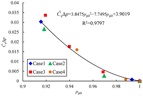
Figure 3.
Fitting diagram of the relationship between gas fields ĈeΔp and ppD.
3. Results and Discussion
3.1. Verification against Field Case
The classic Anderson L reservoir was selected to verify the reliability of the method. The reservoir space is mainly composed of secondary pores with a few fractures, the structural types of it include complex faults and anticlinal structures. It is a typical weakly elastic water-drive abnormally high-pressured condensate gas reservoir. The initial formation pressure of the reservoir is 65.548 MPa, the burial depth is 3403.7 m, the irreducible water saturation of the formation is 0.35, and the compressibility of formation rock and irreducible water are 2.176 × 10⁻³ MPa−1 and 4.410 × 10⁻³ MPa−1, respectively. The gas production data are shown in Table 3.
Table 3.
Historical production data of the Anderson L gas reservoir.
To compare the characteristics and reliability of different methods, we took the calculation results of the volumetric method as the true value of calculation, and compared the reserves calculation methods in this paper and the literature with the volumetric method to calculate the relative errors. Table 4 lists part of the calculation results.
Table 4.
Comparison of dynamic reserves estimation results of different methods.
A comparison of the calculation results in the Table 4 reveals the following findings:
- The errors of the methods that can be applied to the early dynamic reserves calculation in the literature were too large, which proves the necessity of correction. The error of the calculation results of Equations (16) and (25) was 5.59% and 4.88%, respectively; therefore, Equations (16) and (25) were feasible;
- Among all the methods that can be used in the early dynamic reserves calculations, Equation (16) had the highest accuracy with a weak aquifer, and Equation (25) had a higher accuracy with a strong aquifer. More importantly, these methods are simple in form and convenient in calculation, which has stronger practicality.
3.2. Validation against Case
In this section, the proposed new dynamic reserves evaluation method is validated by B-15 well in the Amu Darya gas reservoir in Turkmenistan as an example. The validation case was taken from the Callovian-Oxfordian Stage of the Middle and Upper Jurassic carbonate gas field on the right bank of the Amu Darya, Turkmenistan. The reservoir space is mainly composed of secondary pores and fractures which are extensively developed. The initial formation pressure of well B-15 is 54.34 MPa; the burial depth of the reservoir is 3100 m; the initial pressure coefficient is 1.80; and the aquifer ratio is 13. Presently, the formation pressure is 46.557 MPa, and the pressure coefficient is 1.53. The production history data for well B-15 since production are shown in Table 5 and the current degree of recovery is close to 70%.
Table 5.
Historical production data of well B-15.
Bourgoyne (1990) [33] proposed a method for calculating binomial reserves. Through fitting results, it was found that the method had multiple solutions, and the error between two different formulas could not be ignored (Figure 4). The regression factors were a1 = 0.6528, b1 = 0.0371, a2 = 0.6144, and b2 = 0.0466; the geological reserves were G1 = 26.857 × 10⁸ m3 and G2 = 24.935 × 10⁸ m3. This finding shows that the method does suffer from a high degree of ambiguity when applied to early reservoir development.
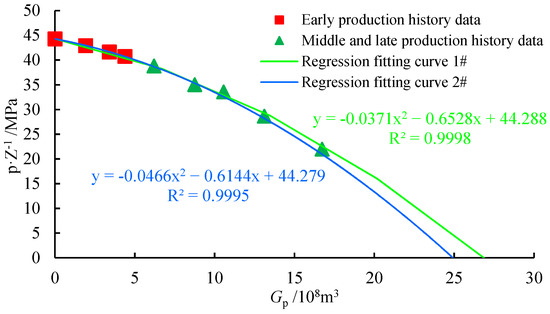
Figure 4.
Pressure decline diagram of the methods of Bourgoyne (1990).
The pseudo reserves correction method was utilized for the calculation, and the virtual dynamic reserves were calculated as Gpes = 55.007 × 10⁸ m3 according to the fitting of Equation (11) (Figure 5), and the final real dynamic reserves were Greal-a = 25.766 × 10⁸ m3 after correction according to Equation (16). We used abnormally high-pressured reservoirs for the whole period production data to verify the accuracy of Equation (16) and the real dynamic reserves were Greal-b = 25.473 × 10⁸ m3. Then, we found that the method used linear extrapolation, it was less likely to cause error accumulation, and it was suitable for the calculation of early dynamic reserves.
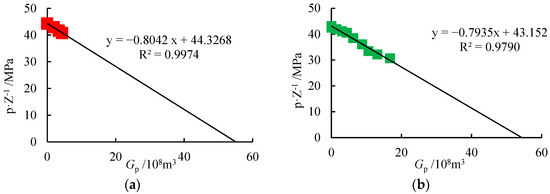
Figure 5.
Pressure decline diagram of the pseudo reserves correction method in well B-15. (a). Early historical production data; (b) Historical production data for the whole period.
The relationship curve between F and Et was drawn (Figure 6) according to Equation (17), fitting the gas field dynamic reserves G = 24.254 × 10⁸ m3; the current cumulative water influx was We = 1.2 × 10⁵ m3.
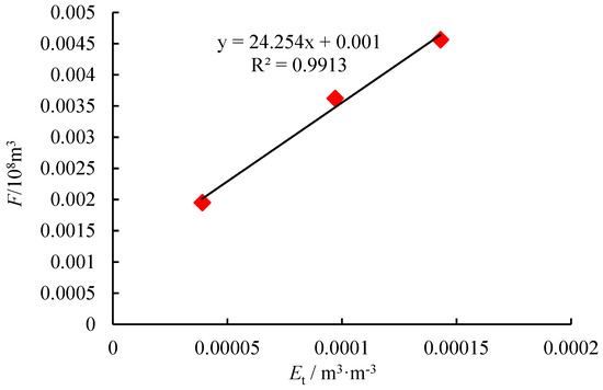
Figure 6.
Well-controlled dynamic reserves estimation fitting diagram of well B-15.
3.3. Discussion
In this paper, we showed the different calculation results by Equation (11), (16), (17), and Bourgoyne’s Model (Figure 7). Among them, Bourgoyne’s Model showed ambiguity in the early dynamic reserves calculation, and the error of each solution could not be ignored. Therefore, Bourgoyne’s Model is not suitable for the dynamic reserves calculation from mid to late development. However, both Equation (16) and Equation (17) had preferable accuracy. When calculating the dynamic reserves of gas reservoirs, Equation (16) mainly considered the influence of the abnormally high-pressure effect (ĈeΔp), and Equation (17) mainly considered the influence of water influx. Therefore, Equation (16) is recommended when the abnormal high-pressure effect dominates in the early stage, and Equation (17) is recommended when the edge and bottom water invade in the late stage. When calculating dynamic gas reservoir reserves with different aquifer ratios, we recommend Equation (16) for a weak aquifer ratio and recommend Equation (17) for a strong aquifer ratio.
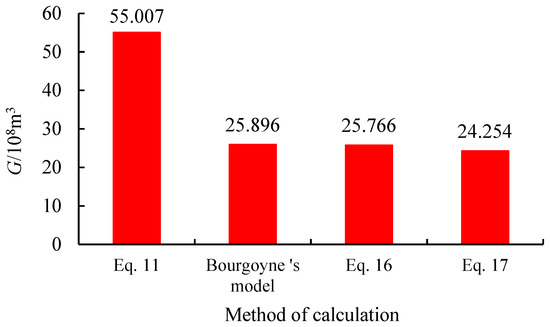
Figure 7.
Comparison diagram of dynamic reserves obtained by three kinds of methods.
When the abnormally high-pressure effect is not considered, the calculation results in Figure 7 showed that Equation (11) was 52.9% and 53.2% above the Bourgoyne’s Model and Equation (16), respectively, indicating that the abnormally high-pressure effect cannot be disregarded. With the different aquifer size ratios, Equation (17) was 6.8% and 6.2% below Bourgoyne’s Model, and Equation (16), respectively; therefore, the aquifer size ratio cannot be underestimated in well-controlled dynamic reserves calculations.
In conclusion, the influence of the abnormally high-pressure effect should be considered in the early calculation of gas reservoir dynamic reserves in the development process of abnormally high-pressured edge and bottom water reservoirs. The influence of water influx should be considered when calculating the dynamic reserves of gas reservoirs.
4. Conclusions
- (1)
- A new reserves estimation method was proposed for dynamic reserves estimation of abnormally high-pressured reservoirs with edge and bottom water influx. The problem of an abnormally pressure effect was addressed by solving the inflection point problem of the traditional virtual reserves correction method. The problem of water influx was resolved by fitting the empirical formulas between ĈeΔp and ppD, and the formulas for the dynamic reserves and water influx of the rearranged gas reservoir were obtained. These methods are simpler in form and more applicable;
- (2)
- With a weak aquifer ratio, the boundary point between the abnormally high-pressured stage and normally pressure stage of edge and bottom water reservoir development was the pressure coefficient, which was equal to 1.2. In the abnormally high-pressured stage, the pressure correction term ĈeΔp was approximately linearly negatively related to the corresponding pressure coefficient α;
- (3)
- Field cases showed that the calculated reserves by the newly proposed reserves estimation method were in accordance with actual reserves estimation methods. In the field case in Anderson L, the relative errors of the two new methods of dynamic reserves calculation were 5.59% and 4.88%, which demonstrated that the dynamic reserves estimation method was effective in abnormally high-pressured reservoirs;
- (4)
- In the field case of the Amu Darya B reservoir, the influence of the abnormally pressure effect on the dynamic reserves calculation was 52.9% and 53.2%, which mainly affected the dynamic reserves calculation of the early stage. The effect of the water influx on the dynamic reserves calculation was 6.8% and 6.2%, which mainly affected the dynamic reserves calculation of the late stage.
Author Contributions
Conceptualization, Y.C. and X.L.; Formal analysis, Y.C. and X.L.; Funding acquisition, Y.C. and C.T.; Investigation, C.G. and T.L.; Methodology, Y.C. and C.G.; Project administration, Y.C. and T.L.; Software development, X.L.; Visualization, Y.C. and C.G.; Writing-original draft Y.C.; Writing—review and editing Y.C. All authors have read and agreed to the published version of the manuscript.
Funding
The authors would like to appreciate the PetroChina Technological Research Project (2021DJ3301); Scientific Research Project of the Shaanxi Provincial Department of Education, China (20JK0848).
Institutional Review Board Statement
Not Applicable.
Informed Consent Statement
Not Applicable.
Data Availability Statement
The datasets generated and/or analyzed during the current study are available from the corresponding author on reasonable request.
Conflicts of Interest
The authors declare that they have no known competing financial interests or personal relationships that could have appeared to influence the work reported in this paper.
Appendix A
Table A1.
Historical production data of the N. Ossun reservoir [33].
Table A1.
Historical production data of the N. Ossun reservoir [33].
| Number | p/MPa | Z | Gp/108 m3 | α |
|---|---|---|---|---|
| 1 | 61.52 | 1.473 | 0.00 | 1.65 |
| 2 | 61.00 | 1.465 | 0.19 | 1.63 |
| 3 | 57.39 | 1.400 | 0.93 | 1.54 |
| 4 | 51.15 | 1.288 | 2.94 | 1.37 |
| 5 | 47.44 | 1.219 | 4.41 | 1.27 |
| 6 | 41.82 | 1.130 | 6.79 | 1.12 |
| 7 | 37.86 | 1.075 | 7.89 | 1.01 |
| 8 | 32.97 | 0.967 | 9.54 | 0.88 |
| 9 | 28.3 | 0.887 | 11.36 | 0.76 |
Table A2.
Historical production data of the Louis. Offshore reservoir [20].
Table A2.
Historical production data of the Louis. Offshore reservoir [20].
| Number | p/MPa | Z | Gp/108 m3 | α |
|---|---|---|---|---|
| 1 | 78.92 | 1.496 | 0.00 | 1.99 |
| 2 | 73.61 | 1.438 | 2.81 | 1.85 |
| 3 | 69.86 | 1.397 | 8.10 | 1.76 |
| 4 | 63.81 | 1.330 | 15.18 | 1.61 |
| 5 | 59.13 | 1.280 | 21.99 | 1.49 |
| 6 | 54.52 | 1.230 | 28.72 | 1.37 |
| 7 | 50.89 | 1.192 | 34.08 | 1.28 |
| 8 | 47.22 | 1.154 | 41.06 | 1.19 |
| 9 | 44.05 | 1.122 | 45.49 | 1.11 |
| 10 | 40.18 | 1.084 | 51.63 | 1.01 |
| 11 | 37.30 | 1.057 | 55.99 | 0.94 |
Table A3.
Historical production data of the Stafford reservoir [20].
Table A3.
Historical production data of the Stafford reservoir [20].
| Number | p/MPa | Z | Gp/108 m3 | α |
|---|---|---|---|---|
| 1 | 49.65 | 1.184 | 0.00 | 1.83 |
| 2 | 48.10 | 1.167 | 0.20 | 1.78 |
| 3 | 46.35 | 1.148 | 0.43 | 1.71 |
| 4 | 44.34 | 1.126 | 0.70 | 1.64 |
| 5 | 42.98 | 1.112 | 0.94 | 1.59 |
| 6 | 43.06 | 1.113 | 1.04 | 1.59 |
| 7 | 40.94 | 1.091 | 1.21 | 1.51 |
| 8 | 39.44 | 1.076 | 1.47 | 1.46 |
| 9 | 36.87 | 1.050 | 1.72 | 1.36 |
| 10 | 31.18 | 0.999 | 2.35 | 1.15 |
| 11 | 25.32 | 0.956 | 3.01 | 0.93 |
| 12 | 21.49 | 0.935 | 3.47 | 0.79 |
| 13 | 19.55 | 0.928 | 3.73 | 0.72 |
Table A4.
Historical production data of the GOM reservoir [33].
Table A4.
Historical production data of the GOM reservoir [33].
| Number | p/MPa | Z | Gp/108 m3 | α |
|---|---|---|---|---|
| 1 | 84.48 | 1.6869 | 0.00 | 2.18 |
| 2 | 81.03 | 1.6394 | 0.11 | 2.09 |
| 3 | 76.13 | 1.5719 | 0.24 | 1.96 |
| 4 | 71.72 | 1.5108 | 0.38 | 1.85 |
| 5 | 66.89 | 1.444 | 0.52 | 1.72 |
| 6 | 65.10 | 1.4192 | 0.65 | 1.68 |
| 7 | 61.58 | 1.3705 | 0.77 | 1.59 |
| 8 | 59.65 | 1.3439 | 0.93 | 1.54 |
| 9 | 56.13 | 1.3268 | 1.08 | 1.45 |
| 10 | 52.55 | 1.2784 | 1.23 | 1.35 |
| 11 | 49.10 | 1.2329 | 1.38 | 1.26 |
| 12 | 46.69 | 1.2017 | 1.51 | 1.20 |
| 13 | 41.72 | 1.139 | 1.70 | 1.07 |
Table A5.
Historical production data of the Miocene S. Louis reservoir [33].
Table A5.
Historical production data of the Miocene S. Louis reservoir [33].
| Number | p/MPa | Z | Gp/108 m3 | α |
|---|---|---|---|---|
| 1 | 75.75 | 1.489 | 0.00 | 2.27 |
| 2 | 57.33 | 1.272 | 0.82 | 1.72 |
| 3 | 48.71 | 1.174 | 1.55 | 1.46 |
| 4 | 43.10 | 1.170 | 1.77 | 1.29 |
| 5 | 33.96 | 1.078 | 2.12 | 1.02 |
References
- Oscar, M.O.; Fernando, S.V.; Jorge, A.V.; Arévalo, V.J.A. Advances in the production mechanism diagnosis of gas reservoirs through material balance studies. In Proceedings of the SPE Annual Technical Conference and Exhibition, Houston, TX, USA, 26–29 September 2004. [Google Scholar] [CrossRef]
- Zhang, L.X.; He, Y.X.; Guo, C.Q.; Yang, Y. Dynamic material balance method for estimating gas in place of abnormally high-pressured gas reservoirs. Lithosphere 2021, 2021, 6669012. [Google Scholar] [CrossRef]
- Lyu, X.; Zhu, G.; Liu, Z. Well-controlled dynamic hydrocarbon reserves calculation of fracture–cavity karst carbonate reservoirs based on production data analysis. J. Petrol. Explor. Prod. Technol. 2020, 10, 2401–2410. [Google Scholar] [CrossRef]
- Zhang, Y.; Ge, H.; Zhao, K. Simulation of pressure response resulted from non-uniform fracture network communication and its application to interwell-fracturing interference in shale oil reservoirs. Geomech. Geophys. Geo-Energy Geo-Resour. 2022, 8, 114. [Google Scholar] [CrossRef]
- Johnson, N.L.; Currie, S.M.; Ilk, D.; Blasingame, T.A. A simple methodology for direct estimation of gas-in-place and reserves using rate-time data. In Proceedings of the SPE Rocky Mountain Petroleum Technology Conference, Denver, CO, USA, 14–16 April 2009. [Google Scholar] [CrossRef]
- Kabir, C.S.; Parekh, B.; Mustafa, M.A. Material-balance analysis of gas reservoirs with diverse drive mechanisms. In Proceedings of the SPE Annual Technical Conference and Exhibition, Society of Petroleum Engineers, Houston, TX, USA, 28–30 September 2015. [Google Scholar] [CrossRef]
- Miao, Y.; Zhao, C.; Zhou, G. New rate-decline forecast approach for lowpermeability gas reservoirs with hydraulic fracturing treatments. J. Petrol. Sci. Eng. 2020, 190, 107112. [Google Scholar] [CrossRef]
- King, G.R. Material-balance techniques for coal-seam and devonian shale gas reservoirs with limited water Influx. SPE Reserv. Eng. 1993, 8, 67–72. [Google Scholar] [CrossRef]
- Walsh, M.P. Discussion of Application of material balance for high pressure gas reservoirs. In Proceedings of the SPE Gas Technology Symposium, Calgary, AB, Canada, 28 April–1 May 1996. [Google Scholar] [CrossRef]
- Pletcher, J.L. Improvements to reservoir material-balance methods. SPE Reserv. Eval. Eng. 2002, 5, 49–59. [Google Scholar] [CrossRef]
- Sun, Z.; Shi, J.; Zhang, T.; Wu, K.; Miao, Y.; Feng, D.; Sun, F.; Han, S.; Wang, S.; Hou, C.; et al. The modified gas-water two phase version flowing material balance equation for low permeability CBM reservoirs. J. Petrol. Sci. Eng. 2018, 165, 726–735. [Google Scholar] [CrossRef]
- Zhang, Y.J.; Ge, H.K.; Shen, Y.H. Evaluating the potential for oil recovery by imbibition and time-delay effect in tight reservoirs during shut-in. J. Pet. Sci. Eng. 2019, 184, 106557. [Google Scholar] [CrossRef]
- Chen, Y.Q.; Hu, J.G. A new method for determining geological reserves and effective compression factors in abnormally high-pressured gas reservoirs. Gas Ind. 1993, 13, 53–58. [Google Scholar]
- Gonzales, F.E.; Ilk, D.; Blasingame, T.A. A quadratic cumulative production model for the material balance of an abnormally pressured gas reservoir. In Proceedings of the SPE Western Regional and Pacific Section AAPG Joint Meeting, Bakersfield, CA, USA, 31 March–2 April 2008. [Google Scholar] [CrossRef]
- Li, C.L. Study on the calculation method of water intrusion in gas reservoirs. Xinjiang Pet. Geol. 2003, 430–431. [Google Scholar]
- Feng, G.Q.; Liu, C.D.; Ran, L.; Xiao, M.H. Comparison of reserves calculation methods for abnormally high-pressured gas reservoirs. J. Chongqing Univ. Sci. Technol. (Nat. Sci. Ed.) 2010, 12, 13–16. [Google Scholar] [CrossRef]
- Ding, X.F.; Liu, Z.B.; Pan, D.Z. New method for calculating geological reserves and cumulative effective compression factor of abnormally high-pressured gas reservoirs. Acta Pet. Sin. 2010, 31, 626–628, 632. [Google Scholar]
- Bian, X.Q.; Du, Z.M.; Chen, J. Binomial material balance equation predicts reserves in abnormally high-pressured gas reservoirs. J. Southwest Pet. Univ. (Sci. Technol. Ed.) 2010, 32, 75–78. [Google Scholar] [CrossRef]
- Jiao, Y.W.; Xia, J.; Liu, P.C.; Zhang, J.; Li, B.Z.; Tian, Q.; Wu, Y.P. New material balance analysis method for abnormally high-pressured gas-hydrocarbon reservoir with water influx. Int. J. Hydrogen Energy 2017, 42, 18718–18727. [Google Scholar] [CrossRef]
- Ramagost, B.P.; Farshad, F.F. P/Z abnormally pressured gas reservoirs. In Proceedings of the SPE Annual Technical Conference and Exhibition, San Antonio, TX, USA, 4–7 October 1981. [Google Scholar] [CrossRef]
- Roach, R.H. Analyzing Geopressured Reservoirs—A Material Balance Technique; Unsolicited paper; SPE: Richardson, TX, USA, December 1981. [Google Scholar]
- Fetkovich, M.J.; Reese, D.E.; Whitson, C.H. Application of a general material balances for high-pressure gas reservoirs. SPE J. 1991, 3, 3–13. [Google Scholar] [CrossRef]
- Yale, D.P.; Nabor, G.W.; Russell, J.A. Application of variable formation compressibility for improved reservoir analysis. In Proceedings of the SPE Annual Technical Conference and Exhibition, Houston, TX, USA, 3–6 October 1993. [Google Scholar] [CrossRef]
- Wang, S.W.; Stevenson, V.M.; Ohaeri, D.H. Analysis of overpressured reservoirs with a new material balance method. In Proceedings of the SPE Annual Technical Conference and Exhibition, Houston, TX, USA, 3–6 October 1999. [Google Scholar] [CrossRef]
- Rahman, N.M.A.; Anderson, D.M.; Mattar, L. New, rigorous material balance equation for gas flow in a compressible formation with residual fluid saturation. In Proceedings of the SPE Gas Technology Symposium, Calgary, AB, Canada, 15–17 May 2006. [Google Scholar] [CrossRef]
- Zhang, J.Z.; Gao, T.R. Compressibility of abnormally-pressured gas reservoirs and its effect on reserves. ACS Omega 2021, 6, 26221–26230. [Google Scholar] [CrossRef] [PubMed]
- Zhang, Y.; Zou, Y.; Zhang, Y. Experimental Study on Characteristics and Mechanisms of Matrix Pressure Transmission Near the Fracture Surface During Post-Fracturing Shut-In in Tight Oil Reservoirs. J. Pet. Sci. Eng. 2022, 219, 111133. [Google Scholar] [CrossRef]
- Liao, Y.T. Regression equation for calculating natural water influx. Oil Explor. Dev. 1990, 1, 71–74. [Google Scholar]
- Yang, E.L.; Zhang, J.G.; Song, K.P.; Huang, B. Numerical simulation study of low permeability gas reservoir at Daqing five stations. Gas Ind. 2008, 3, 102–104, 147–148. [Google Scholar] [CrossRef]
- Wang, Z.H.; Wang, Z.D.; Zeng, F.H.; Guo, P.; Xu, X.Y.; Deng, D. The material balance equation for fractured vuggy gas reservoirs with bottom water-drive combining stress and gravity effects. J. Nat. Gas Sci. Eng. 2017, 44, 96–108. [Google Scholar] [CrossRef]
- Xue, T.; Ji, Y.; Cheng, L.B.; Lv, C.S.; Yang, Y.X.; Lan, Z.K. A new method for determining dynamic storage capacity and water energy in water-driven gas reservoirs. In Petroleum Geology & Oilfield Development in Daqing; CNKI, Tongfang Knowledge Network Technology Co., Ltd.: Beijing, China, 2022; pp. 1–6. [Google Scholar] [CrossRef]
- Carter, R.D.; Tracy, G.W. An improved method for calculating water influx. Trans. AIME 1960, 219, 415–417. [Google Scholar] [CrossRef]
- Bourgoyne, A.T., Jr. Shale Water as a Pressure Support Mechanism in Gas Reservoirs Having Abnormal Formation Pressure. J. Pet. Sci. 1990, 3, 305. [Google Scholar] [CrossRef]


Disclaimer/Publisher’s Note: The statements, opinions and data contained in all publications are solely those of the individual author(s) and contributor(s) and not of MDPI and/or the editor(s). MDPI and/or the editor(s) disclaim responsibility for any injury to people or property resulting from any ideas, methods, instructions or products referred to in the content. |
© 2023 by the authors. Licensee MDPI, Basel, Switzerland. This article is an open access article distributed under the terms and conditions of the Creative Commons Attribution (CC BY) license (https://creativecommons.org/licenses/by/4.0/).