Abstract
A non-Newtonian stagnation point fluid flow towards two different inclined heated surfaces is mathematically formulated with pertinent effects, namely mixed convection, viscous dissipation, thermal radiations, heat generation, and temperature-dependent thermal conductivity. Mass transfer is additionally considered by the use of a concentration equation. The flow narrating equations are solved numerically by using the shooting method along with the Runge–Kutta scheme. A total of 80 samples are considered for five different inputs, namely the velocities ratio parameter, temperature Grashof number, Casson fluid parameter, solutal Grashof number, and magnetic field parameter. A total of 70% of the data are used for training the network; 15% of the data are used for validation; and 15% of the data are used for testing. The skin friction coefficient (SFC) is the targeted output. Ten neurons are considered in the hidden layer. The artificial networking models are trained by using the Levenberg–Marquardt algorithm. The SFC values are predicted for cylindrical and flat surfaces by using developed artificial neural networking (ANN) models. SFC shows decline values for the velocity ratio parameter, concentration Grashof number, Casson fluid parameter, and solutal Grashof number. In an absolute sense, owning to a prediction by ANN models, we have seen that the SFC values are high in magnitude for the case of an inclined cylindrical surface in comparison with a flat surface. The present results will serve as a helpful source for future studies on the prediction of surface quantities by using artificial intelligence.
1. Introduction
It is well acknowledged that the physics of non-Newtonian fluid flows poses a unique challenge to scientists, mathematicians, and engineers. There is not a single constitutive equation that demonstrates all of the characteristics of such non-Newtonian fluids due to the complexity of these fluids. Many non-Newtonian fluid models have been put out along the process. Among these, the Casson fluid [1] has drawn a lot of interest. In the Casson fluid, the yield stress is present. It is well known that Casson fluid is a shear-thinning fluid [2,3] and it behaves like a solid when the yield stress is more than the shear stress, but it begins to move in the case of large shear stress [4]. The following are examples of Casson fluid: jelly, soup, tomato sauce, concentrated fruit liquids, honey, etc. Casson fluids can also be used to examine the properties of human blood. Owning to such importance, various studies are performed to inspect the Casson fluid in different physical frames. For example, Kelessidis and Maglione [5] used the Casson flow field to see if they could adequately characterize the rheology of bentonite suspensions by using twelve sets of experiments. For all rheological models, equations were provided that made it possible to calculate the actual shear rates that the fluids inside the rotational viscometer experienced. Using real and Newtonian shear rates, which were frequently employed in the study of rheometric data, non-linear regression was used to derive the two rheological parameters for the Casson model. The findings demonstrated that both models provide adequate statistical indicators for describing the experimental data of these bentonite suspensions. Additionally, the study demonstrated that real shear rates for both models were consistently larger than Newtonian shear rates. According to the specific suspension, the discrepancies were greater at low shear rates and became less at higher shear rates. The rheograms’ forms principally remained the same, showing that the rheological parameters calculated using actual shear rates were quite close to those calculated using Newtonian shear rates. The computation of the rheological parameters for both models and both methodologies further supported this. Kelessidis and Maglione [5] derived the differences in yield by using true shear rates, which were, at most, 7% for the Casson model and, at most, 3% for the plastic viscosity. However, given that there are mathematical methods that allow for the use of actual shear rates with no compromise, these minor discrepancies do not support the use of Newtonian shear rates. Mahanta and Shaw [6] introduced a convective condition at the surface where the fluid’s thermal conductivity varied linearly with respect to temperature to provide a magnetohydrodynamic (MHD) three-dimensional Casson fluid flow via a porous linearly stretched sheet. The velocity and temperature fields were computed for a variety of factors. The governing equations were resolved with the help of the spectral relaxation method (SRM). When the current findings were compared to currently available, limited solutions, they showed good agreement with one another and with many criteria. To study the behaviors with various settings, graphs for the temperature and velocity were plotted. For various parameters, the impact of skin friction on the local Nusselt number was addressed and provided in tabular form. The magnetized fluid across a channel was studied by Akbar et al. [7]. For the purpose of simulating fluid viscoplastic behavior, the reliable Casson model was used. The direction of the fluid flow was at an angle to the external magnetic field. Effects of viscous dissipation were included. The metachronal waves that were propagated as cilia beat on the channel’s inner walls and regulated the flow. They proposed a closed form solution. Additionally, a comparison with Newtonian fluids was performed. To see the phenomenon of trapping, streamlines were drawn. The calculations showed that, near the channel walls, velocity increases with rising Hartmann number magnitude; however, a considerable slowing was seen in the core flow region. Thammanna et al. [8] considered three-dimensional Casson fluid flow with various physical effects. Similarity variables were used to drop the order, and the resulting equation was solved by the Runge–Kutta scheme. The data were then shown graphically for concentration, temperature, and velocity toward several relevant physical parameters. The results showed that the Casson parameter’s bigger values reduced the velocity components. In contrast, the thickness of the solutel boundary layer decreased as the Schmidt number and chemical reaction parameter were increased. When the current results and the already available limiting solutions were evaluated, they were found to be in good agreement. Siddiqa et al. [9] conducted a boundary layer analysis to examine the impact of non-linear surface radiation on Casson fluid past a vertical wavy cone. The boundary conditions were expressed using the Stefan–Boltzmann formula to express the contribution of surface radiative heat flux. The governing equations were first transformed into a non-dimensional, non-conserved form using the proper sets of transformations, and then a numerical method was employed to find the solutions. Graphical representations of our numerical findings were presented while key non-dimensional parameters varied. Additionally, a comparison with the existing literature was made, and it was found that the results were generally in agreement. Additionally, high values of the Casson rheological parameter significantly influence fluid velocity, although temperature profiles exhibit the reverse trend. Mahmood et al. [10] conducted a numerical examination of Casson nanofluid flow, heat transmission, and entropy formation over a stretching surface. Various physical effects are included in the simplified flow model. The controlling nonlinear partial differential equations were reduced by using the similarity technique. The solutions for the temperature, velocity, and entropy profiles were then approximately determined by solving the resulting set using a finite difference numerical technique. Additionally, the boundary’s heat exchange rate and skin friction factor were computed and graphically visualized. The key results included the detrimental effects of Lorentz forces within the boundary layer as well as the rise in temperature caused by rising non-Newtonian, thermal radiation and sheet convection parameters.
Madhu et al. [11] examined the Casson flow field in a square porous cavity. The top wall was assumed to be adiabatic, and the temperature control within the cavity was achieved by cooling of the side walls and heating of the bottom wall. The governing equations of a flow problem were obtained and solved by using the penalty finite element approach. It was investigated how varying heated zone lengths, Rayleigh numbers, and Darcy numbers affected the cavity’s flow and temperature distribution. Investigations were conducted into how changing a fluid’s effective viscosity might affect heat transfer and fluid flow. The obtained results demonstrate that heat transfer and flow circulation increased for Casson fluid parameter and Darcy number. The flow of Casson fluid past an exponentially expanding curved surface with convective boundary conditions were examined by Kumar et al. [12]. It was supposed that the fluid motion was laminar and time-dependent. The impacts of varied heat source/sink, Joule heating, temperature-dependent thermal conductivity, and thermal radiation were evaluated. In order to solve the governing partial differential equations numerically, using techniques such as shooting and the Runge–Kutta method, the appropriate transformations were taken into consideration. The effect of different dimensionless parameters on the fields of velocity and temperature were depicted in graphs, and it was found that the temperature field was improved by the thermal conductivity, radiation, and heat parameters. Banerjee et al. [13] investigated the Casson fluid flow in a diverging channel with a porosity effect. The flow field was investigated by using nonlinear coupled equations. Additionally, numerical solutions were achieved by using the MATLAB software “bvp4c”. The study shows that only boundary layer flow was possible if mass suction exceeded a threshold that was dependent on the Casson parameter. Additionally, the temperature distribution was significantly impacted by the rheological characteristics of the viscous dissipation, and, as a result, the temperature within the boundary layer region is lower than the temperature of the free stream. Parvin et al. [14] discussed Casson flow field with various physical effects. The mixed convection, shrinkage parameter, Dufour number, and Soret number were some of the physical parameters that the model was subjected to. Moreover, the inclined magnetic field and an angled shrinking sheet were applied to this model. The reduced ordinary differential equations’ final numerical solutions were obtained using the MATLAB bvp4c program as the primary mathematical tool. The governing partial differential equations give rise to these ODEs. For specific values of the physical parameters, numerical representations were created for the skin friction coefficient.
Obalalu et al. [15] demonstrated, theoretically and numerically, the squeezed Casson fluid flow with thermal radiation. The model was governed by a differential system, which was achieved. The following observations were made as a result of the analysis. They discovered that the presence of squeeze numbers is crucial and that increasing the squeezing parameter raises the fluid temperature. Skin friction was significantly affected by higher values of variable viscosity. Raza et al. [16] examined the heat transfer in Casson nanofluid towards a vertical plate. The leading equations with physical attributes of nanoparticles were established, and the Laplace transformation was used to report the solution. It was determined that the velocity increases with the Grashof number. When compared to the Caputo–Fabrizio fractional derivative, the results exhibit a greater declining tendency. The effects of Lorentz forces on the Casson fluid flow of a water-based Fe3O4-MWCNT hybrid nanofluid caused by dust particles from a stretching sheet was examined by Saeed et al. [17]. By using similarity variables, the leading PDEs (partial differential equations) were converted into ODEs (ordinary differential equations), and the converted ODEs were then given an exact solution. In-depth consideration was given to the effects of several physical limitations, such as the magnetic parameter and Casson parameter, on the fluid velocity and dust velocity for normal nanofluid and hybrid nanofluid. Recent attempts to examine Casson fluid in numerous configurations can be accessed in Refs. [18,19,20].
The thermophysical properties of heat transfer in fluid science have many applications, including electronic cooling, heat exchangers, refrigeration systems, thermal distillation systems, steam–electric power generation, solar collectors, and spacecraft thermal protection, to name a few. This is widely agreed upon by researchers in the field of thermal engineering. Considering such importance, we offer numerical values of skin friction coefficient at both flat and cylindrical surfaces in the presence of various effects, namely, an externally applied magnetic field, a stagnation point, mixed convection, thermal radiation, viscous dissipation, and heat generation. To be more specific, the non-Newtonain fluid flow towards two inclined surfaces along with the aspects of heat and mass transfer are considered simultaneously. The shooting method and Runge–Kutta (RK) scheme are used to solve the flow equations of the problem. The ANN model is trained by using the Levenberg–Marquardt technique. The skin friction coefficient values at both surfaces are debated by the use of the ANN model. The article is designed as follows: Section 1 is devoted to a literature survey on Casson fluid flow subject to various configurations. The flow field formulation is presented in Section 2. A directory for the solution scheme is given in Section 3, while Section 4 contains the construction of the ANN model. The obtained results and discussion are offered in Section 5. The outcomes are summarized in Section 6.
2. Mathematical Formulation
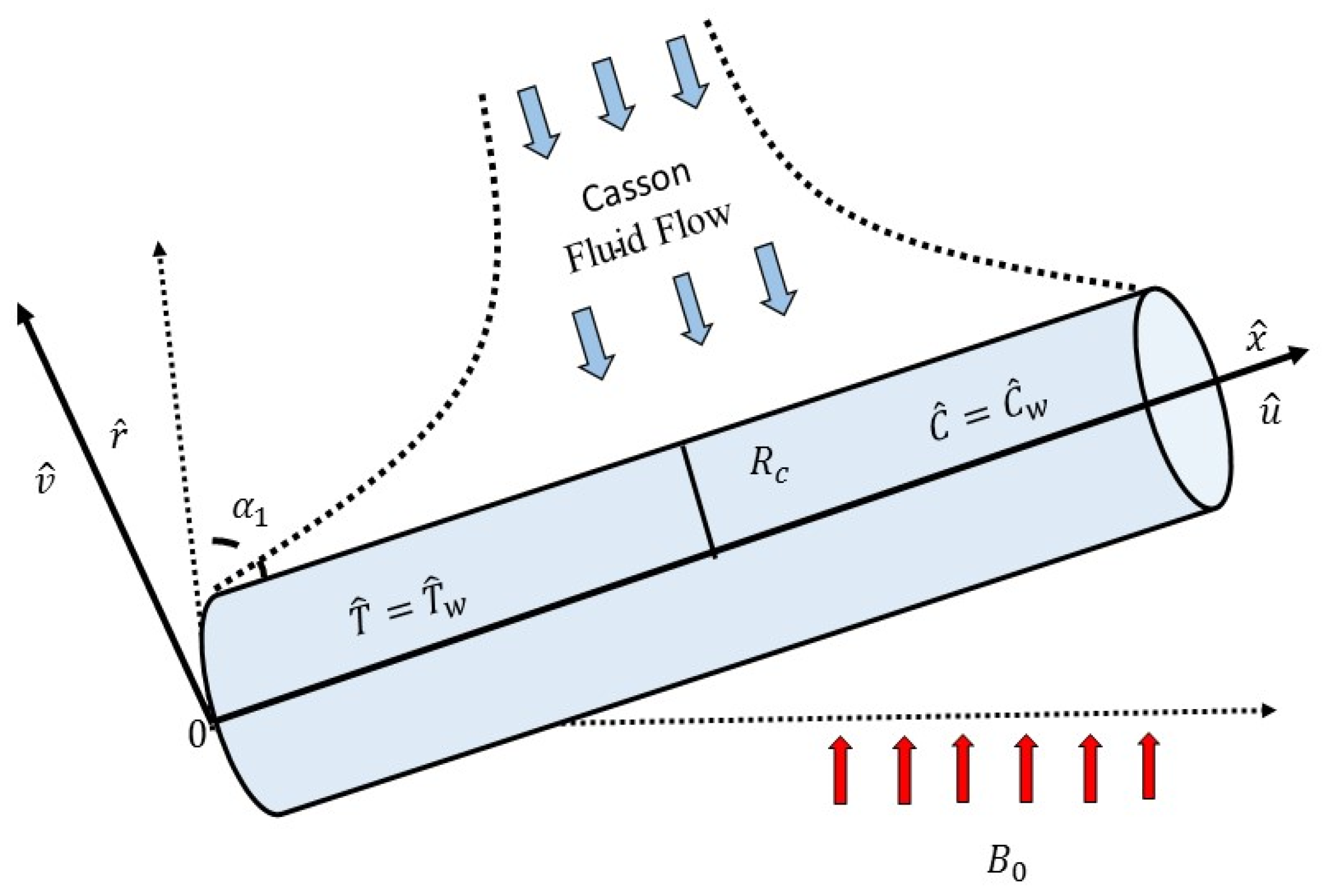
The non-Newtonian fluid flow is introduced by means of stretching inclined surfaces, namely, cylinder and plate. The flow regime is strengthened by considering the magnetic field, stagnation point flow, temperature-dependent conductivity, viscous dissipation, mixed convection, and heat generation. The mass transfer is considered by entreating the concentration equation. The magnetic field is applied perpendicular to the Casson fluid flow. The strength of both concentration and temperature is considered higher at the surface as compared to strength far away from the surface. The geometry of the problem is offered as Figure 1. The ultimate Casson fluid flow equations [21] for the present problem can be written as:

Figure 1.
Geometry of the problem [21].
The flux (radioactive) is well-defined as:
The thermal conductivity is defined as
The conditions given on borderline are:
Here, stands for radius of cylinder, is kinematic viscosity, denotes the coefficient of solutal expansion, are concentration, temperature, fluid density, heat generation coefficient, and mass diffusivity, respectively. Our interest is to examine the comparative impact of flow parameters on Casson fluid flow towards both flat and cylindrical surfaces by use of an artificial neural networking model. Therefore, for the solution of Equations (1)–(4), we need to transform such PDEs into equivalent ODEs. For such purpose we consider:
In light of Equation (8), Equations (1)–(3) turn into
and the conditions reduce to:
The dimensionless temperature, concentration, and velocity are denoted by , respectively. The parameters are mathematically summarized as follows:
The Eckert number, Prandtl number, solutal Grashof number, thermal Grashof number, thermal radiation parameter, Casson fluid parameter, Schmidt number, and velocities ratio parameter are denoted by . The fluid is flowing over the stretching cylindrical and flat surfaces, and, hence, the skin friction exists. The SFC is formulated as follows:
3. Solution Scheme
The reduced order equations, namely Equations (9)–(11), are coupled and non-linear, which makes it difficult to solve them analytically. Various solution techniques [22,23,24,25,26] are used to report the flow differential equations, but to obtain the best approximate numerical solution, the shooting method will be used. The shooting approach [27,28] has been shown to be effective and practical for solving boundary value problems (BVP). In order to apply the shooting approach, the BVP must first be transformed into an initial value problem (IVP), after which initial value predictions are made. Iterative solutions are then used to solve the IVPs, and this process is repeated until the boundary conditions are satisfied. The Newton–Raphson method is utilized for initial value estimate while the Runge–Kutta formula is employed for iterative calculations. The necessary step is to have an initial value system, and it can be created by assuming:
Owing Equation (15) into Equations (9)–(11) results in
While conditions reduces to
Results from the self-coding of the aforementioned equations in Matlab are displayed as line graphs (velocity plots) and tabular data (skin friction coefficient).
4. Construction of Artificial Neural Networking Model
The non-Newtonian fluid flow towards two different stretched surfaces is considered and modelled mathematically. The flow equations are solved numerically. The skin friction coefficient is evaluated at a flat plate (Model-I) and cylindrical surface (Model-II). For both cases, the ANN models are constructed to forecast the values of skin friction at surfaces.
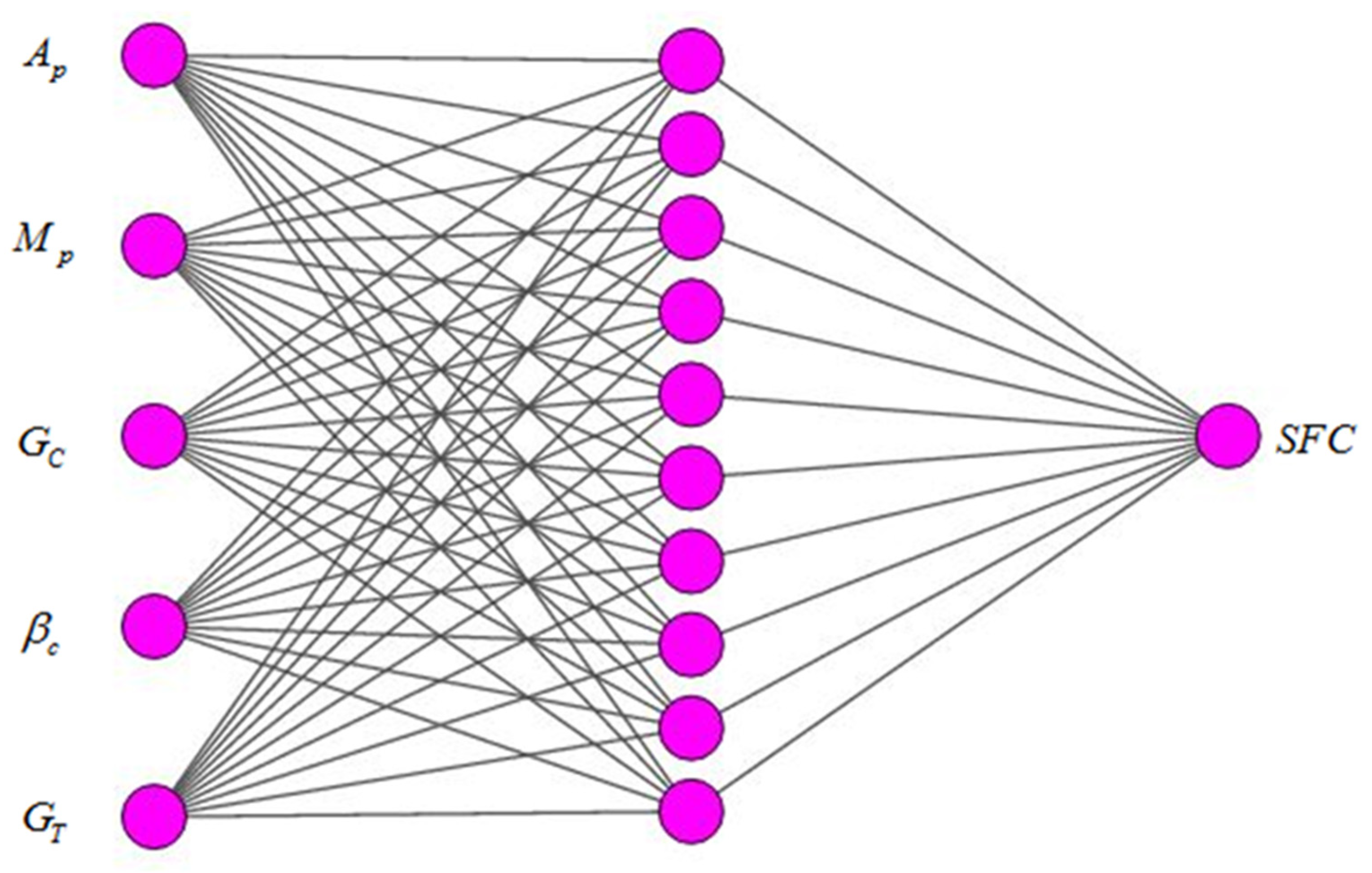
It is strongly believed by researchers that the artificial neural networking model [29,30,31,32] in alliance with multilayer perceptron (MLP) has great learning ability and is thus used to predict various physical phenomena. The three different layers are used in MLP networks. The inputs are used in the first layer while the centrally involved layer is termed the hidden layer. The last layer is termed as output layer and prediction data is held by this layer. The architecture of the network model is offered in Figure 2.
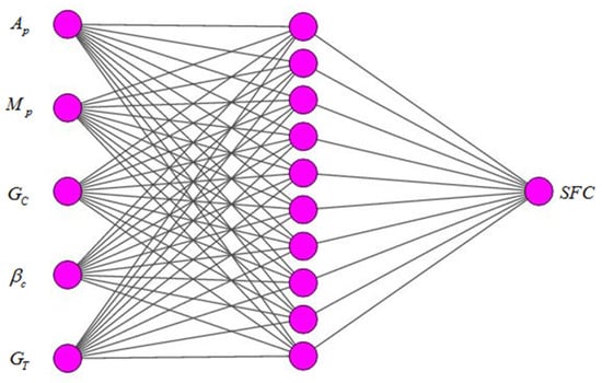
Figure 2.
Architecture of network model.
We have constructed two ANN models, namely ANN Model-I and II. ANN Model-I is constructed to predict the skin friction coefficient at a flat surface while ANN Model-II is constructed to offer a prediction of SFC values at a cylindrical surface. For both ANN models, the five different flow parameters are used as inputs while the SFC is considered as output. The flow parameters are velocity ratio, magnetic field parameters, concentration Grashof number, Casson fluid parameter, and temperature Grashof number. The symbolic information for two different models is given in Table 1. For 5 inputs, we have collected 80 different samples (positive values) and, hence, 80 sample values for skin friction coefficient. A total of 70% of the data are used for training the network; 15% of the data are used for validation; and 15% of the data are used for testing. The complete information in this regard is offered in Table 2. The ten neurons are considered in the hidden layer, and the Levenberg–Marquardt technique is used to train the network. The mathematical expressions of the transfer functions used in hidden and output layers are written as:
Pureline(x) = x.

Table 1.
Input and output details for ANN models.
Table 2.
Data description for ANN models.
For performance examination of artificial neural networking models of skin friction coefficient at flat and cylindrical surfaces, we have considered the following parameters, namely, the mean squared error (MSE) and coefficient of determination (R). The mathematical equations used in the calculation of the performance parameters are written as:
5. Results and Discussion
The Casson fluid flow towards two different stretched surfaces is examined by use of artificial neural networking models. In detail, the Casson flow over a stretching cylinder is mathematically formulated and solved by the use of the shooting method. The Casson fluid flow over a flat surface is evaluated by considering the zero-value of the curvature parameter. The ultimate flow parameters involved in this direction are the velocity ratio parameter, concentration Grashof number, magnetic field parameter, Casson fluid parameter, and temperature Grashof number. We have evaluated the SFC at the cylindrical surface towards these parameters. The range of parameters is selected by owning the convergence of the numerical scheme.
Table 3, Table 4, Table 5, Table 6, Table 7, Table 8, Table 9 and Table 10 are strategized in this direction. In detail, Table 3 offered the SFC at both flat and cylindrical surfaces. Such evaluation is conducted for the magnetized frame. In an absolute sense, we noticed that, for higher values of the velocity ratio parameter, the SFC declines significantly.
Table 3.
Variation in SFC for .
Table 4.
Variation in SFC for when .
Table 5.
Variation in SFC for [21].
Table 6.
Variation in SFC for when [21].
Table 7.
Variation in SFC for .
Table 8.
Variation in SFC for when .
Table 9.
Variation in SFC for [21].
Table 10.
Variation in SFC for when [21].
Further, we see that the strength of SFC at the cylinder is higher than SFC at a flat surface. Table 4 gives the numerical data of SFC at flat and cylindrical surfaces in the absence of a magnetic field.
We observed that the SFC shows a declining nature for the velocities ratio parameter. The strength of SFC is greater in the case of the cylinder surface. Table 5 offers the impact of the concentration Grashof number on SFC for both surfaces when an externally applied magnetic field is present.
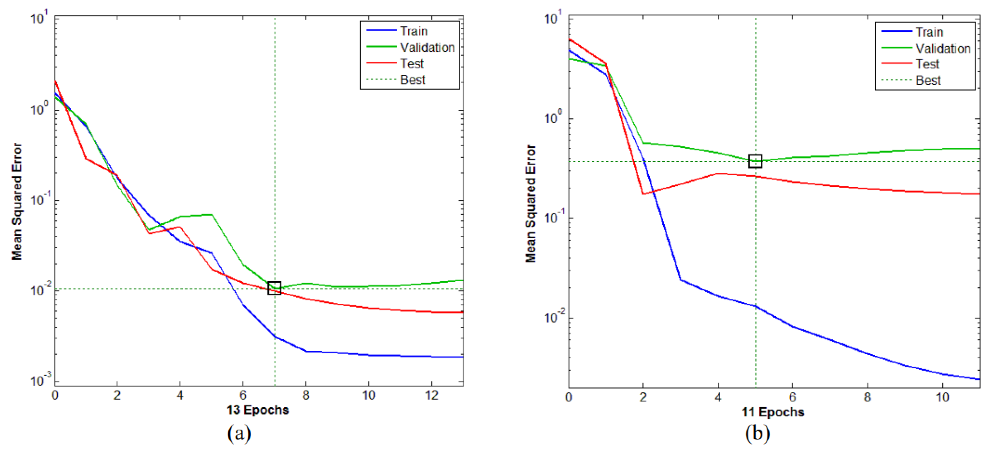
We have seen that the SFC decrease for concentration Grashof number, and the observation is the same for both surfaces. The magnitude of the skin friction coefficient is higher for the cylinder [21]. Table 6 offers the effect of the concentration Grashof number on SFC for both surfaces in the absence of a magnetic field. The SFC is found the decreasing function of the concentration Grashof number. Such trends are similar for both surfaces [21]. Table 7 concludes the examination of SFC towards the Casson fluid parameter for the magnetized flow regime. For both surfaces, we see that SFC reduces significantly for the Casson fluid parameter. Table 8 offers the SFC values for both surfaces in the absence of a magnetic field. We observed that SFC values decrease as the Casson fluid parameter increases. Comparing a flat plate to a cylindrical surface, the SFC magnitude is larger. Table 9 and Table 10 offer examination on the impact of temperature Grashof number on the SFC [21]. To be more specific, Table 9 offers the impact of temperature Grashof number on SFC when we considered externally applied magnetic field while Table 10 offers the SFC values for the absence of a magnetic field. For both cases, we have seen that the SFC shows decline values towards positive values of temperature Grashof number. Further, the magnitude of SFC is higher in the case of a stretched cylindrical surface. We have developed two different artificial neural networking models (ANN-I and ANN-II) for SFC of Casson fluid flow at two surfaces, namely flat and cylindrical surfaces. ANN-I owns the Casson flow at a flat surface while ANN-II owns the Casson fluid flow at a cylindrical surface. The training of the network is one of the important stops to developing the artificial neural networking model. We have used the Levenberg–Marquardt algorithm to train the network. Figure 3a,b offer the training performances of the ANN models. In detail, Figure 3a offers the training performance of ANN model for prediction of SFC at a flat surface while Figure 3b gives the training performance of the ANN model for the prediction of SFC at a cylindrical surface. In the context of an MLP network’s training cycle (epoch), it is important to note that, for ANN-I, the best validation performance is 0.01067 at epoch 7, and, for ANN-II, the best validation performance is 0.37089 at epoch 5. For both graphs, we observed that initial values of MSE are high and decrease towards developed stages. Figure 4a,b offers the error histogram of ANN models being constructed to predict the values of SFC. In detail, Figure 4a offers the error histogram of ANN model-I for a flat surface while Figure 4b offer the error histogram of ANN model-II for the cylindrical surface. Both error histograms are with 20 Bins. We have seen that the error values for both ANN models are reasonably low, and, hence, the training stages of ANN-I and ANN-II to estimate SFC at a flat surface and a cylindrical surface are completed ideally.
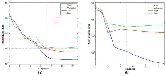
Figure 3.
(a) Training performance of ANN model for flat surface; (b) Training performance of ANN model for cylindrical surface.
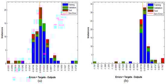
Figure 4.
(a) Error histogram of ANN model for flat surface; (b) Error histogram of ANN model for cylindrical surface.
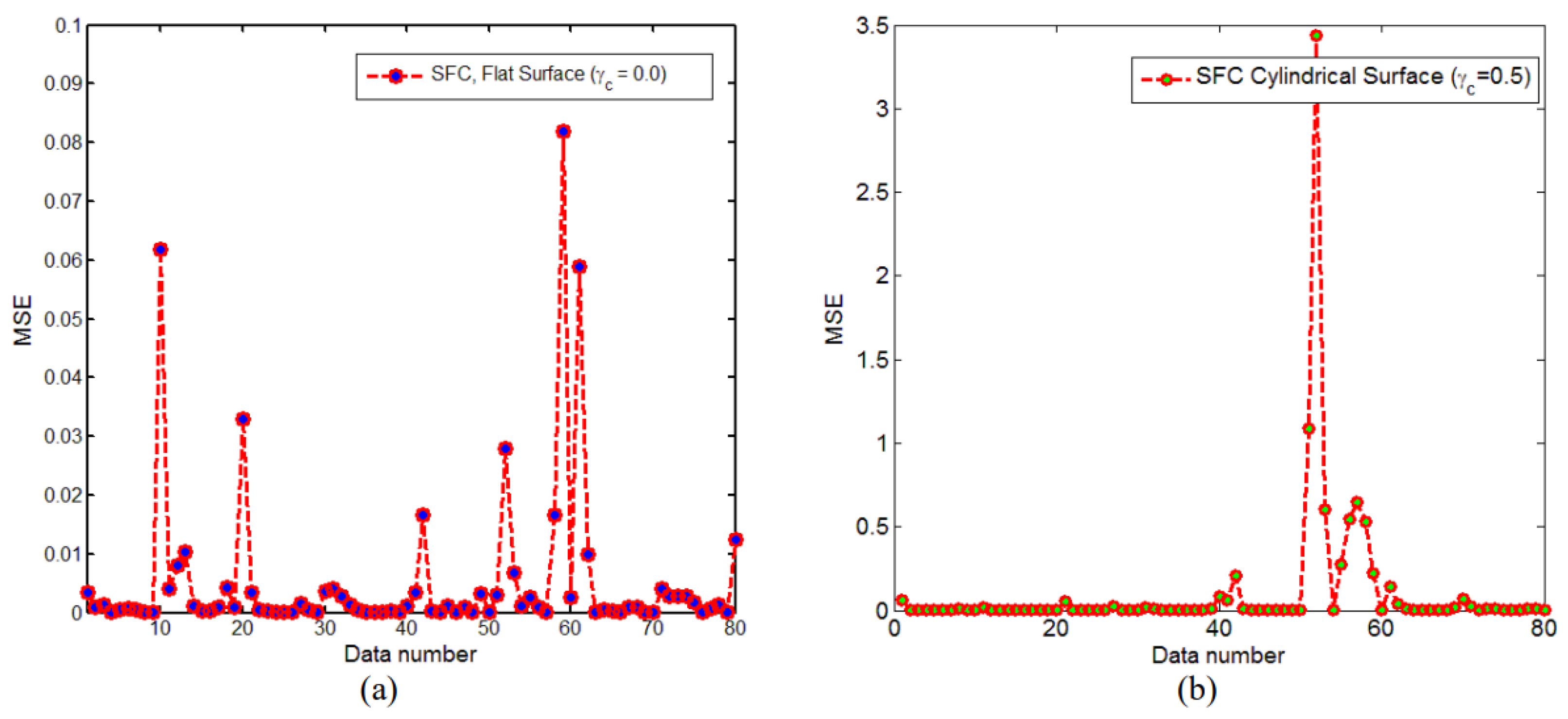
Figure 5a,b offer the mean square error graphs of SFC. To be more specific, Figure 5a offers the MSE for SFC at the flat surface while Figure 5b offers the MSE for SFC at the cylindrical surface. Both figures support that the learning stages of ANN-I and ANN-II are completed in a perfect way. MSE values are plotted for each of the 80 data samples. The nearness of MSE values towards zero reflects the fewer errors while training the ANN models to predict the SFC. The average MSE for the case of a flat surface is 0.0051666569 while, for the case of a cylindrical surface, it is recorded as 0.101813. Which is quite low, hence, the training of the neural networking model is perfect to predict the values of SFC at both flat and cylindrical surfaces.
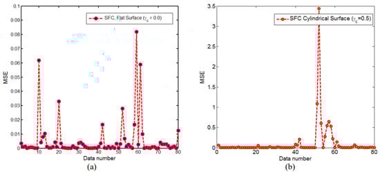
Figure 5.
(a) MSE for SFC at plat surface; (b) MSE for SFC at cylindrical surface.
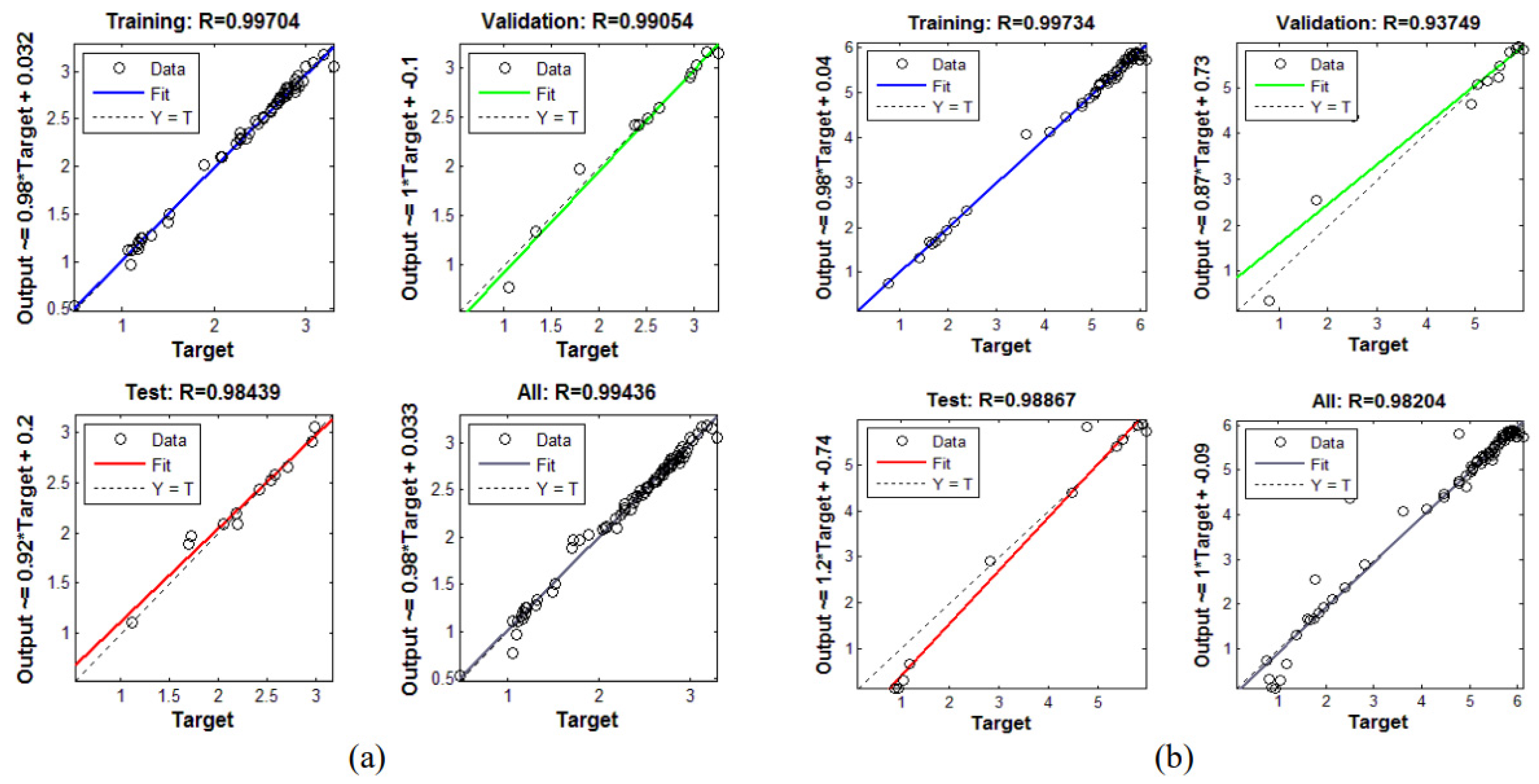
Figure 6a,b offer the regression values of SFC data for flat and cylindrical surfaces, respectively. It is important to note that the regression value offers the correlation between targets and prediction values, and, if it is close to one, we can say we have a close relationship. For the case of a flat plate, the regression value was R = 0.99704. For validation, it was recorded as R = 0.99054. Further, at the testing stage, we noticed R = 0.98439. Collectively, the regression value for the case of a flat surface was R = 0.99436. As far as the case of the cylindrical surface is concerned, we obtained R = 0.99734, R = 0.93749, and R = 0.9867 for the training, validation, and testing stages. The collective value for the case of cylindrical surface was R = 0.98204. Owning all these statistics from Figure 6a,b, we can conclude that the constructed ANN-I and ANN-II are the best models to predict the SFC at both surfaces.
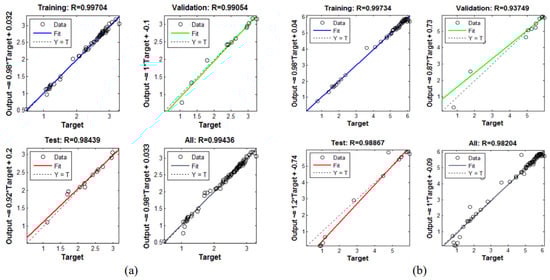
Figure 6.
(a) Regression values for SFC data at flat surface; (b) Regression values for SFC data at cylindrical surface.
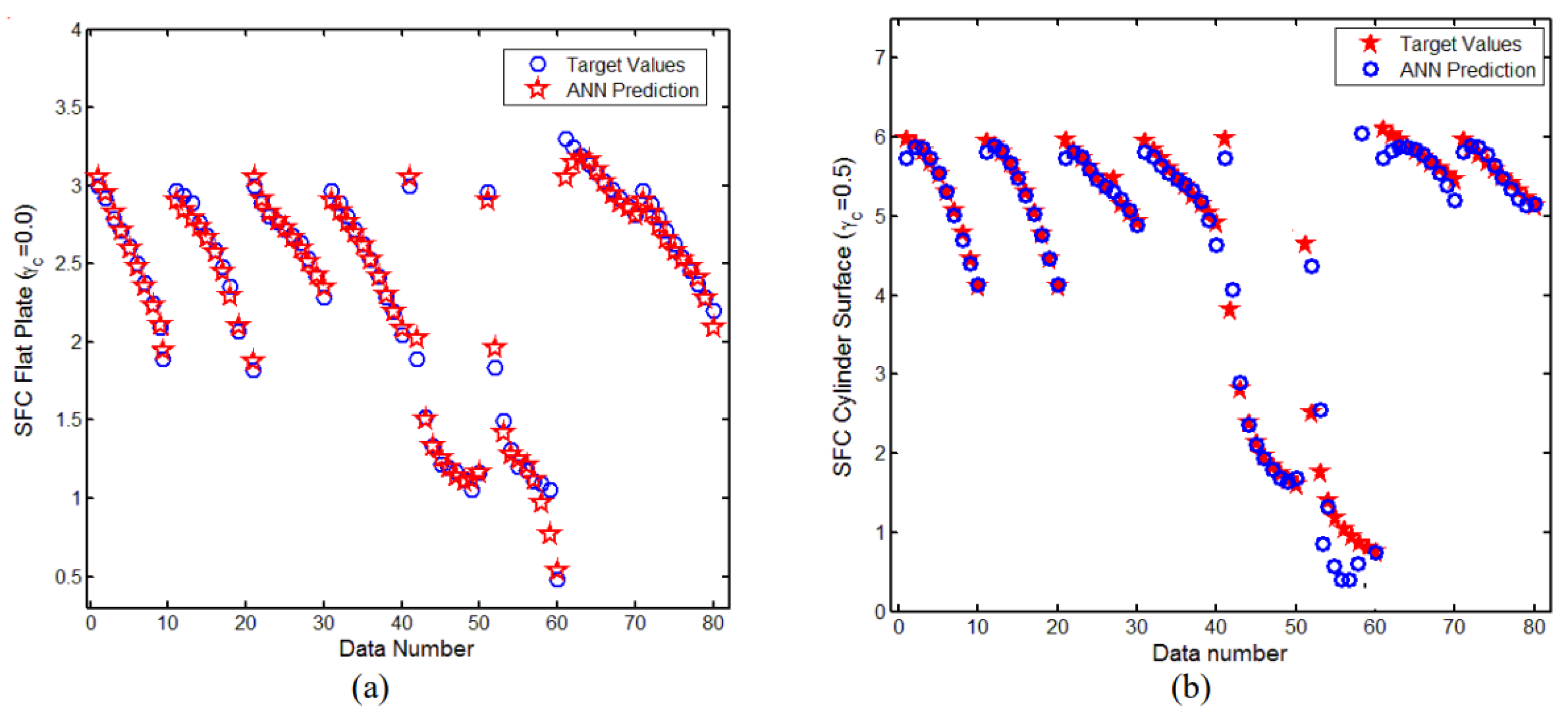
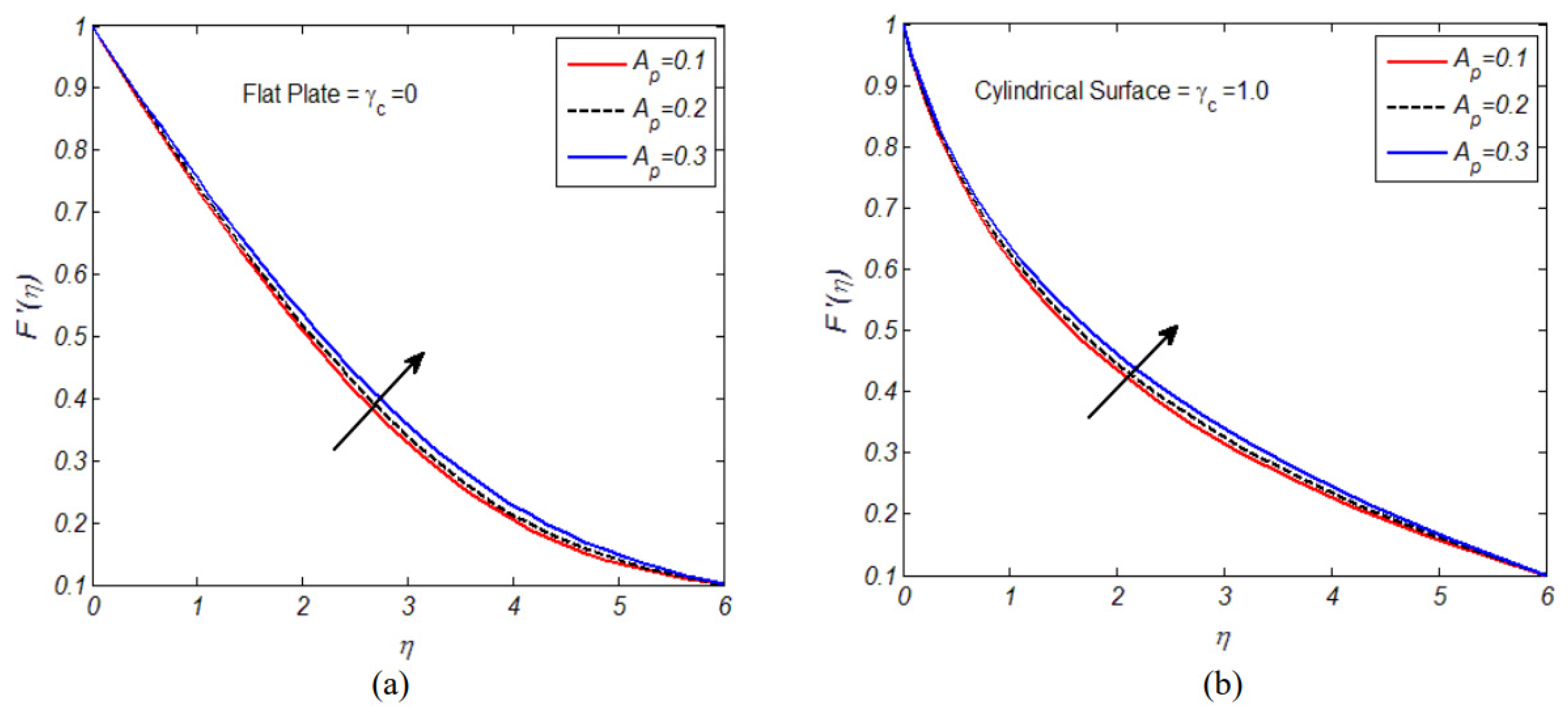
Figure 7a,b offer the comparison of actual values of SFC and predicted values of SFC by artificial neural networking model. In detail, Figure 7a offers the comparison of ANN and target data set for a flat surface while Figure 7b gives the comparison of ANN and target data set for the cylindrical surface. We can observe from both figures that the majority of ANN model outputs are in good agreement with the SFC target values. Owning such overlap, we can say that the developed models, namely ANN-I and ANN-II, can predict SFC with high accuracy. Figure 8a,b offer the impact of positive variation of the velocities ratio parameter on Casson fluid velocity. In detail, Figure 8a gives the velocities ratio parameter impact on velocity for the case of the flat surface while Figure 8b provides the velocities ratio parameter impact on velocity for the case of the cylindrical surface. It is seen that Casson fluid velocity admits direct relation towards the velocities ratio parameter. It is significant to remember that the velocity ratio parameter displays the proportion between the free stream and the Casson fluid stretching velocity. When the ratio parameter is smaller than one, it is assumed that the stretching velocity plays a more significant role than the free stream. The sloped surfaces significantly disrupt fluid flow as a result.
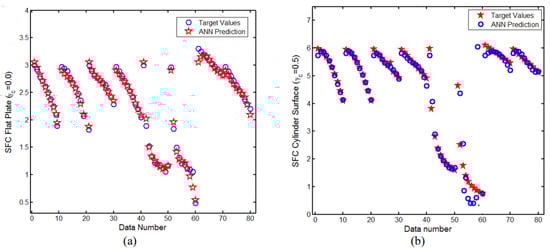
Figure 7.
(a) Estimation of ANN and target data set for flat surface; (b) Estimation of ANN and target data set for cylindrical surface.
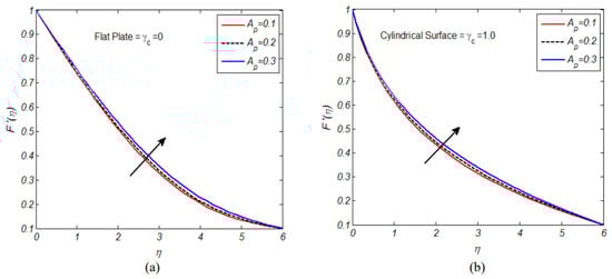
Figure 8.
(a) Impact of on velocity at flat surface; (b) Impact of on velocity at cylindrical surface.
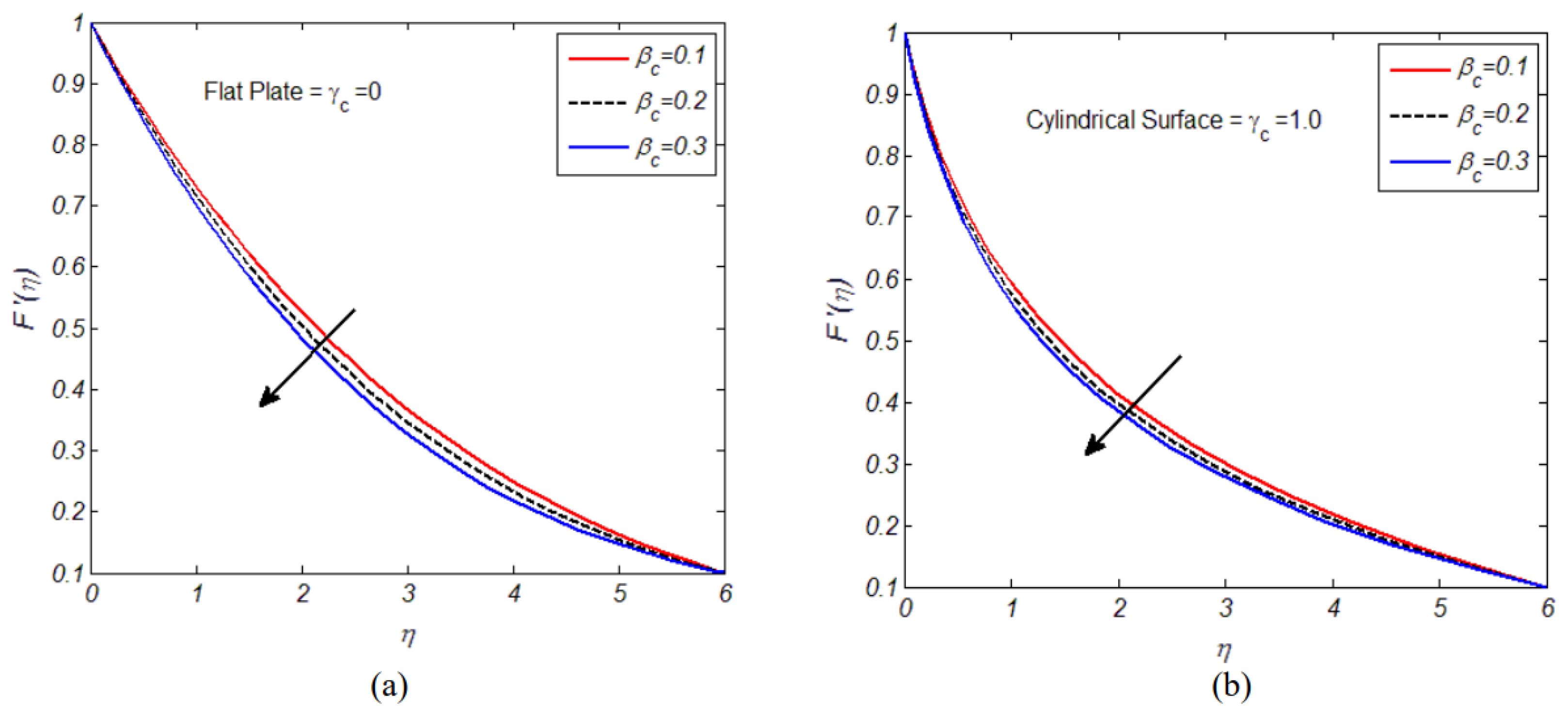
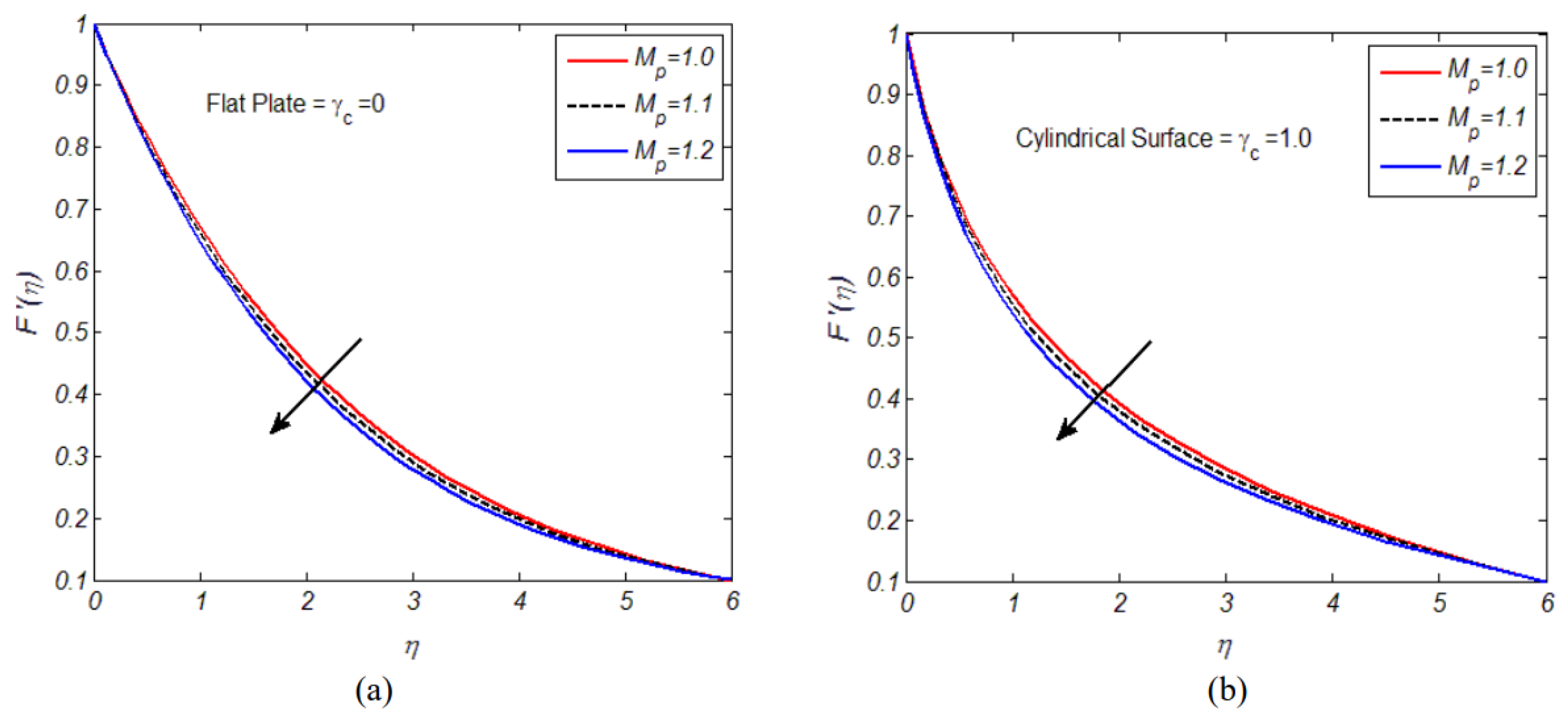
Figure 9a,b offer the influence of the Casson fluid parameter on Casson fluid velocity. In detail, Figure 9a contributes the Casson fluid parameter effect on fluid over a flat surface while Figure 9b gives the impact of the Casson fluid parameter on fluid over a cylindrical surface. We have seen that Casson fluid velocity admits indirect relation towards fluid parameter. The influence of magnetic field parameter on Casson fluid velocity over a flat and cylindrical surface is inspected. Figure 10a,b are evidence in this direction. In detail, Figure 10a reports the magnetic field parameter impact on velocity, and we noticed that velocity decreases as the magnetic field parameter increases. Similarly, Figure 10b offers the impact of magnetic parameter on velocity over a stretching cylinder and we noticed that fluid velocity shows decline trends for variation in magnetic field parameter. For positive values of magnetic field parameter, the Lorentz force increases, and, as a result, resistance towards fluid flow increases, which ultimately brings a decline in fluid velocity over stretched surfaces. Table 11 offers the performance particulars for both artificial neural networking models, and one can see that the developed models have the capacity to predict the skin friction coefficient values at both flat and cylindrical surfaces with high accuracy. In the absence of an externally applied magnetic field, heat generation, and mass transfer, the present problem reduces to the research problem given by Hayat et al. [33]. The skin friction coefficient (SFC) is considered a comparison quantity towards two important flow parameters, namely, the curvature parameter and the Casson fluid parameter. Owing to Table 12, we found an excellent match.
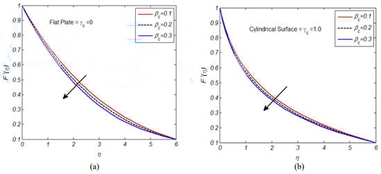
Figure 9.
(a) Impact of on velocity at flat surface; (b) Impact of on velocity at cylindrical surface.
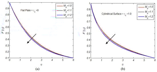
Figure 10.
(a) Impact of on velocity at flat surface; (b) Impact of on velocity at cylindrical surface.
Table 11.
Performance grades for constructed ANN models.
Table 12.
Comparison of SFC with Hayat et al. [33].
6. Conclusions
The non-Newtonian fluid flow towards cylindrical and flat inclined surfaces was examined by the use of ANN models. The flow was carried with a stagnation point, mixed convection, externally applied magnetic field, thermal radiations, viscous dissipation, heat generation, and temperature-dependent thermal conductivity. The flow was mathematically formulated and solved by the use of the shooting method. The skin friction coefficient was evaluated at both surfaces towards five, unlike flow variables. The SFC was predicted for both surfaces by using ANN models. The results are as follows:
- The values of the coefficient of determination are in support of the best artificial neural networking to predict the SFC at the surface.
- The average mean square error (MSE) value for the ANN model towards a flat stretched surface was 0.51666569% and it was quite satisfactory.
- Owning to a prediction by ANN models, we observed that, compared to a flat surface, the strength of the SFC was larger in the case of cylindrical surfaces.
- SFC showed decline values for the velocity ratio parameter, the concentration Grashof number, the Casson fluid parameter, and the solutal Grashof number.
- Casson fluid velocity showed increasing trends towards the velocity ratio parameter; the opposite was the case for the Casson fluid parameter and magnetic field parameter.
- One can extend this study to examine the non-Newtonian fluid models (namely Power Law, the Carreau, and the Generalized Power Law) subject to stretched surfaces having engineering standpoints.
Author Contributions
Methodology, K.U.R.; Software, K.U.R.; Validation, K.U.R.; Formal analysis, W.S.; Data curation, W.S.; Writing – original draft, K.U.R.; Supervision, W.S. All authors have read and agreed to the published version of the manuscript.
Funding
This research received no external funding.
Data Availability Statement
Not applicable.
Acknowledgments
The authors would like to thank Prince Sultan University for their support through the TAS research lab.
Conflicts of Interest
The authors declare no conflict of interest.
Nomenclature
| Cylindrical coordinates | |
| Kinematic viscosity | |
| Velocity components | |
| Casson fluid parameter | |
| Gravitational acceleration | |
| Thermal expansion coefficient | |
| Angle of inclination | |
| Solutal expansion coefficient | |
| Temperature of fluid | |
| Ambient temperature | |
| Magnetic field constant | |
| Ambient concentration | |
| Concentration of fluid | |
| Free stream velocity | |
| Specific heat at constant pressure | |
| Fluid electrical conductivity | |
| Fluid density | |
| Variable thermal conductivity | |
| Radiative heat flux | |
| Dynamic viscosity | |
| Characteristic length | |
| Heat generation coefficient | |
| Small parameter | |
| Surface concentration | |
| Reference velocity | |
| Mass diffusivity | |
| Surface temperature | |
| Radius of cylinder | |
| Fluid concentration | |
| Fluid velocity | |
| Fluid temperature | |
| Concentration Grashof number | |
| Temperature Grashof number | |
| Pr | Prandtl number |
| Radiation parameter | |
| Velocities ratio parameter | |
| Magnetic field parameter | |
| Coefficient of mean absorption | |
| Curvature parameter | |
| Eckert number | |
| Stefan–Boltzmann constant | |
| Sc | Schmidt number |
| Heat generation parameter |
References
- Rohlf, K.; Tenti, G. The role of the Womersley number in pulsatile blood flow: A theoretical study of the Casson model. J. Biomech. 2001, 34, 141–148. [Google Scholar] [CrossRef]
- Mernone, A.; Mazumdar, J.; Lucas, S. A mathematical study of peristaltic transport of a Casson fluid. Math. Comput. Model. 2002, 35, 895–912. [Google Scholar] [CrossRef]
- Joye, D.D. Shear rate and viscosity corrections for a Casson fluid in cylindrical (Couette) geometries. J. Colloid Interface Sci. 2003, 267, 204–210. [Google Scholar] [CrossRef] [PubMed]
- Raja Ramesh, H.; You, Z. Application of the augmented Lagrangian method to steady pipe flows of Bingham, Casson and Herschel–Bulkley fluids. J. Non-Newton. Fluid Mech. 2005, 128, 126–143. [Google Scholar]
- Kelessidis, V.; Maglione, R. Modeling rheological behavior of bentonite suspensions as Casson and Robertson–Stiff fluids using Newtonian and true shear rates in Couette viscometry. Powder Technol. 2006, 168, 134–147. [Google Scholar] [CrossRef]
- Mahanta, G.; Shaw, S. 3D Casson fluid flow past a porous linearly stretching sheet with convective boundary condition. Alex. Eng. J. 2015, 54, 653–659. [Google Scholar] [CrossRef]
- Akbar, N.S.; Tripathi, D.; Bég, O.A.; Khan, Z. MHD dissipative flow and heat transfer of Casson fluids due to metachronal wave propulsion of beating cilia with thermal and velocity slip effects under an oblique magnetic field. Acta Astronaut. 2016, 128, 1–12. [Google Scholar] [CrossRef]
- Thammanna, G.; Kumar, K.G.; Gireesha, B.; Ramesh, G.; Prasannakumara, B. Three dimensional MHD flow of couple stress Casson fluid past an unsteady stretching surface with chemical reaction. Results Phys. 2017, 7, 4104–4110. [Google Scholar] [CrossRef]
- Siddiqa, S.; Begum, N.; Ouazzi, A.; Hossain, A.; Gorla, R.S.R. Heat transfer analysis of Casson dusty fluid flow along a vertical wavy cone with radiating surface. Int. J. Heat Mass Transf. 2018, 127, 589–596. [Google Scholar] [CrossRef]
- Mahmood, A.; Jamshed, W.; Aziz, A. Entropy and heat transfer analysis using Cattaneo-Christov heat flux model for a boundary layer flow of Casson nanofluid. Results Phys. 2018, 10, 640–649. [Google Scholar] [CrossRef]
- Madhu, A.; Chandra, A.; Sharma, S. Natural convection in a partially heated porous cavity to Casson fluid. Int. Commun. Heat Mass Transf. 2020, 114, 104555. [Google Scholar]
- Anantha Kumar, K.; Sugunamma, V.; Sandeep, N. Effect of thermal radiation on MHD Casson fluid flow over an exponentially stretching curved sheet. J. Therm. Anal. Calorim. 2020, 140, 2377–2385. [Google Scholar] [CrossRef]
- Banerjee, A.; Mahato, S.K.; Bhattacharyya, K.; Chamkha, A.J. Divergent channel flow of Casson fluid and heat transfer with suction/blowing and viscous dissipation: Existence of boundary layer. Partial. Differ. Equ. Appl. Math. 2021, 4, 100172. [Google Scholar] [CrossRef]
- Parvin, S.; Mohamed Isa, S.S.; Arifin, N.M.; Md Ali, F. The inclined factors of magnetic field and shrinking sheet in Casson fluid flow, heat and mass transfer. Symmetry 2021, 13, 373. [Google Scholar] [CrossRef]
- Obalalu, A.M.; Ajala, A.O.; Akindele, A.O.; Oladapo, O.A.; Adepoju, O.; Jimoh, M.O. Unsteady squeezed flow and heat transfer of dissipative casson fluid using optimal homotopy analysis method: An application of solar radiation. Partial. Differ. Equ. Appl. Math. 2021, 4, 100146. [Google Scholar] [CrossRef]
- Raza, A.; Khan, S.U.; Farid, S.; Khan, M.I.; Sun, T.-C.; Abbasi, A.; Malik, M. Thermal activity of conventional Casson nanoparticles with ramped temperature due to an infinite vertical plate via fractional derivative approach. Case Stud. Therm. Eng. 2021, 27, 101191. [Google Scholar] [CrossRef]
- Saeed, A.; Algehyne, E.A.; Aldhabani, M.S.; Dawar, A.; Kumam, P.; Kumam, W. Mixed convective flow of a magnetohydrodynamic Casson fluid through a permeable stretching sheet with first-order chemical reaction. PLoS ONE 2022, 17, e0265238. [Google Scholar] [CrossRef]
- Priam, S.S.; Nasrin, R. Numerical appraisal of time-dependent peristaltic duct flow using Casson fluid. Int. J. Mech. Sci. 2022, 233, 107676. [Google Scholar] [CrossRef]
- Prameela, M.; Gangadhar, K.; Reddy, G.J. MHD free convective non-Newtonian Casson fluid flow over an oscillating vertical plate. Partial. Differ. Equ. Appl. Math. 2022, 5, 100366. [Google Scholar] [CrossRef]
- Hussain, S.; Zeeshan, M.; Sagheer, D.-E. Irreversibility analysis for the natural convection of Casson fluid in an inclined porous cavity under the effects of magnetic field and viscous dissipation. Int. J. Therm. Sci. 2022, 179, 107699. [Google Scholar] [CrossRef]
- Rehman, K.U.; Shatanawi, W.; Yaseen, S. A Comparative Numerical Study of Heat and Mass Transfer Individualities in Casson Stagnation Point Fluid Flow Past a Flat and Cylindrical Surfaces. Mathematics 2023, 11, 470. [Google Scholar] [CrossRef]
- Nawaz, Y.; Arif, M.S.; Abodayeh, K.; Mansoor, M. Finite difference schemes for MHD mixed convective Darcy–forchheimer flow of Non-Newtonian fluid over oscillatory sheet: A computational study. Front. Phys. 2023, 11, 1072296. [Google Scholar] [CrossRef]
- Sadaf, H.; Asghar, Z.; Iftikhar, N. Cilia-driven flow analysis of cross fluid model in a horizontal channel. Comput. Part. Mech. 2022, 9, 1–8. [Google Scholar] [CrossRef]
- Nawaz, Y.; Arif, M.S.; Abodayeh, K. Predictor–Corrector Scheme for Electrical Magnetohydrodynamic (MHD) Casson Nanofluid Flow: A Computational Study. Appl. Sci. 2023, 13, 1209. [Google Scholar] [CrossRef]
- Fatima, N.; Kousar, N.; Rehman, K.U.; Shatanawi, W. Magneto-thermal convection in partially heated novel cavity with multiple heaters at bottom wall: A numerical solution. Case Stud. Therm. Eng. 2023, 43, 102781. [Google Scholar] [CrossRef]
- Atashafrooz, M.; Sajjadi, H.; Delouei, A.A. Simulation of Combined Convective-Radiative Heat Transfer of Hybrid Nanofluid Flow inside an Open Trapezoidal Enclosure Considering the Magnetic Force Impacts. J. Magn. Magn. Mater. 2023, 567, 170354. [Google Scholar] [CrossRef]
- Salahuddin, T. Carreau fluid model towards a stretching cylinder: Using Keller box and shooting method. Ain Shams Eng. J. 2020, 11, 495–500. [Google Scholar] [CrossRef]
- Muhammad, K.; Abdelmohsen, S.A.; Abdelbacki, A.M.; Ahmed, B. Ahmed. Darcy-Forchheimer flow of hybrid nanofluid subject to melting heat: A comparative numerical study via shooting method. Int. Commun. Heat Mass Transf. 2022, 135, 106160. [Google Scholar] [CrossRef]
- Shafiq, A.; Çolak, A.B.; Sindhu, T.N.; Muhammad, T.; Shafiq, A.; Çolak, A.B.; Sindhu, T.N.; Muhammad, T. Optimization of Darcy-Forchheimer squeezing flow in nonlinear stratified fluid under convective conditions with artificial neural network. Heat Transf. Res. 2022, 53, 67–89. [Google Scholar] [CrossRef]
- Said, Z.; Sharma, P.; Elavarasan, R.M.; Tiwari, A.K.; Rathod, M.K. Exploring the specific heat capacity of water-based hybrid nanofluids for solar energy applications: A comparative evaluation of modern ensemble machine learning techniques. J. Energy Storage 2022, 54, 105230. [Google Scholar] [CrossRef]
- Acikgoz, O.; Çolak, A.B.; Camci, M.; Karakoyun, Y.; Dalkilic, A.S. Machine learning approach to predict the heat transfer coefficients pertaining to a radiant cooling system coupled with mixed and forced convection. Int. J. Therm. Sci. 2022, 178, 107624. [Google Scholar] [CrossRef]
- Rehman, K.U.; Shatanawi, W.; Çolak, A.B. Artificial Neural Networking Magnification for Heat Transfer Coefficient in Convective Non-Newtonian Fluid with Thermal Radiations and Heat Generation Effects. Mathematics 2023, 11, 342. [Google Scholar] [CrossRef]
- Hayat, T.; Asad, S.; Alsaedi, A. Flow of variable thermal conductivity fluid due to inclined stretching cylinder with viscous dissipation and thermal radiation. Appl. Math. Mech. 2014, 35, 717–728. [Google Scholar] [CrossRef]

Disclaimer/Publisher’s Note: The statements, opinions and data contained in all publications are solely those of the individual author(s) and contributor(s) and not of MDPI and/or the editor(s). MDPI and/or the editor(s) disclaim responsibility for any injury to people or property resulting from any ideas, methods, instructions or products referred to in the content. |
© 2023 by the authors. Licensee MDPI, Basel, Switzerland. This article is an open access article distributed under the terms and conditions of the Creative Commons Attribution (CC BY) license (https://creativecommons.org/licenses/by/4.0/).