Article

Prediction of Oxygen Content in Boiler Flue Gas Based on a Convolutional Neural Network

School of Chemistry, Chemical Engineering and Life Sciences, Wuhan University of Technology, Wuhan 430070, China
*
Author to whom correspondence should be addressed.
Processes 2023, 11(4), 990; https://doi.org/10.3390/pr11040990
Submission received: 7 February 2023 / Revised: 14 March 2023 / Accepted: 20 March 2023 / Published: 24 March 2023

Abstract

:
As one of the core pieces of equipment of the thermal power generation system, the economic and environmental performance of a boiler determines the energy efficiency of the thermal power generation unit. The oxygen content in boiler flue gas is an important parameter reflecting the combustion status of the furnace, and accurate prediction of flue gas oxygen content is of great significance for online boiler optimization. In order to solve the online prediction problem of the oxygen content in boiler flue gas, a CNN is applied to build a time series prediction model, which takes the time series samples within a fixed time window as the input of the model and uses several feature extraction modules containing convolutional, activation, and pooling layers for feature extraction and compression, and the model output is the oxygen content in boiler flue gas. Since the oxygen content in boiler flue gas is not only correlated with other variables but also influenced by its own historical trend, the input of the CNN model is improved, and an oxygen content in boiler flue gas time series prediction model (TS-CNN) is established, which takes the historical values of the boiler flue gas oxygen content as the input of the model. The comparison test results show that the R 2 and R M S E of the TS-CNN model are 0.8929 and 0.1684, respectively. The prediction accuracy is higher than the CNN model, LSSVM model, and BPNN model by 18.6%, 31.2%, and 54.6%, respectively.

1. Introduction

Under the background of China’s “poor in oil, deficient in natural gas, but rich in coal” energy structure, thermal power generation is still an important part of China’s electric power resources production. A boiler is one of the core devices of thermal power generation, and its economic and environmental performance determines the energy efficiency of the whole generator unit [1]. The oxygen content in boiler flue gas is an important parameter that reflects the combustion state of the boiler furnace and is also a key indicator to measure whether the fuel burns adequately. The air/coal ratio required for efficient combustion in the furnace can be reasonably deduced from the oxygen content in the flue gas. Therefore, the timely and accurate measurement of oxygen content in flue gas is of great significance for realizing efficient and stable boiler operation [2,3]. The measurement for oxygen content in boiler flue gas can be divided into direct measurement and soft measurement. At present, zirconia sensors are mostly used to measure the oxygen content in the flue gas in coal-fired power plants in China. However, this method has the disadvantages of moderate lag, decreased measurement accuracy with the aging of sensors, high cost of hardware replacement, short device service life, etc., which struggles to meet the actual needs of power plants [4,5,6].
In recent years, with the continuous development of computer software and hardware, the soft-sensing technology driven by historical data has been widely applied in the fields of boiler combustion optimization, boiler condition monitoring and control, etc. [7,8,9]. Among them, the prediction of oxygen content in boiler flue gas based on modeling methods, such as machine learning, has been studied extensively. Research by Ma [10], Zhang [11], and Geng [12] verified the effectiveness of using the BP neural network and its improved algorithm to establish a soft-sensing model for oxygen content in the flue gas. Su [13], Zhang [14], and Li [15] studied the application of a support vector machine (SVM) and a least squares support vector machine (LS-SVM) in the prediction of oxygen content in boiler flue gas, respectively, and used intelligent optimization algorithms to optimize the parameters of the model, improving the accuracy and stability of the model. However, in this traditional soft-sensing model based on machine learning, the feature that the correlation between the various parameters of boilers will change with different operating conditions is ignored in the selection of modeling variables. In order to solve the above problems, Tang [16,17,18] et al. successively proposed several dynamic correction models for NOx emission concentration of boilers based on an extreme learning machine and a measurement model for oxygen content in flue gas based on a deep belief network. The core idea of their modeling is that there are large differences in the model feature variables under different load conditions, and this method has been verified through comparison.
Compared with traditional machine learning algorithms, deep learning algorithms such as a convolutional neural network (CNN), feedforward neural network, deep belief network, recurrent neural network, and its modified version of long- and short-time memory networks have strong advantages in the learning and expression ability of data characteristics [19,20,21]. A CNN has been successfully applied in the field of boiler combustion process monitoring with complex variables because of its powerful feature extraction and feature expression capabilities. Wang [22], Liu [23], and Han [24] used the convolution operation of the CNN model to extract the flame image features of boiler furnaces and predict the furnace combustion state, boiler combustion efficiency, and other indicators of power plants. However, in the above research, the furnace flame images of the boilers are taken as the input of the model. Before practical application, it is necessary to transform the original boilers to obtain the furnace flame images. For such a boiler system with time delay, high nonlinearity, and multivariable coupling features, the two-dimensional matrix composed of time series samples in a fixed time window can also be used as the object of convolution operation to realize the feature extraction and compression of input sample space on the premise of avoiding variable screening and time delay analysis. Xing [25] et al. converted the historical NOx emission data and boiler combustion process data sample into model training samples and adopted the convolution layer and pooling layer for extraction of input features to establish a NOx emission prediction model based on CNN-LSTM. Taking the time series samples in a fixed time window as the input of the convolutional network, Li [26] and Jia [27] established the NOx emission prediction model and the multi-step prediction model of main steam temperature based on the convolutional neural network, respectively, verifying the effectiveness of the CNN processing timing prediction.
In summary, in this paper, a 130 t/h circulating fluidized bed boiler actually running in a petrochemical enterprise in Shandong is the research object, and in view of the multivariable, nonlinearity, and large time delay characteristics of the boiler, the time series samples in the fixed time window were taken as the input of model, and feature extraction was conducted for input samples by use of convolution operation. On this basis, a prediction model of oxygen content in boiler flue gas based on a convolutional neural network was proposed.

2. Data Acquisition and Analysis

2.1. Data Acquisition

In the SIS system of the power plant, 12,000 historical operation samples of the 130 t/h circulating fluidized bed boiler were collected from 2:19 p.m. on 26 November 2020 to 10:14 a.m. on 29 November 2020. As shown in Table 1, a single sample consists of oxygen content in boiler flue gas and 23 variables. In order to make the established model more consistent with the actual production process, the historical samples collected cover 60–100% of the load conditions, including most of the key variables of the boiler during operation.

2.2. Data Analysis

Boiler operation is a process of multivariable coupling and state accumulation. That is, different operating conditions correspond to different key variables. Moreover, the current state is not simply described as the values of several variables at a certain moment, but the accumulation of states in the past period of time. Generally, the mapping relationship between the input and output of the current system is described in Formulas (1) and (2):
X n = x n l + 1 , 1 x n l + 1 , m x n , 1 x n , m
y n = f X n
However, during the boiler combustion operation, the oxygen content in the boiler flue gas is affected not only by other relevant variables but also by its own historical change trends. Therefore, the mapping relationship between the input and output of the system is revised in Formulas (3) and (4) in this paper:
X n = x n l + 1 , 1 x n l + 1 , m y n l + 1 x n , 1 x n , m y n
y n + 1 = f X n
where X n is a sample set composed of l historical samples of the boiler at the moment n , l is the length of the time window, m is the number of boiler variables, x i , j is the value of the variable i of the sample j , and y i is the oxygen content in the flue gas of the sample n .
The size of X n will increase with the increase in the time window length l , which means a huge scale of input parameters. When such data are processed with a traditional regression learning algorithm, it will take a long time and reduce the generalization performance of the model due to too many parameters to be trained. Therefore, it is necessary to extract the sample features before model training. According to the common variable screening methods, it is often necessary to manually set a threshold and screen the modeling variables based on the correlation between each variable and the target variable. Such methods usually have higher requirements for threshold selection. Different from the above methods, the convolutional neural network can automatically learn the features required for regression tasks from the training sample data, which can improve the model accuracy and training efficiency without relying on the artificial selection of features.

3. Basic Principles of the Convolutional Neural Network

A complete convolutional neural network consists of five basic units: input layer, convolution layer, activation layer, pooling layer, and full connection layer.

3.1. Convolution Layer

The convolution operation is a special feature extraction algorithm that gives practical significance to the convolutional neural network. The convolution layer can extract high-level features with translation invariance from all input parameters through matrix operation and can express the original features effectively. Different from the convolution function in the mathematical sense, for the input matrix A and the convolution kernel of size r × c , the convolution operation is as shown in Formulas (5)–(7), and G i , j is the output matrix.
A = a 1 , 1 a 1 , m a n , 1 a n , m
W = w 1 , 1 w 1 , c w r , 1 w r , c
G i , j = A × W i , j = u = 1 r v = 1 c a i + u 1 , j + v 1 w u , v + b i , j
An example of a two-dimensional convolution operation is shown in Figure 1. The input matrix of the original 4 × 4 is transformed into the output matrix of 3 × 3 under the convolution operation of the convolution kernel that is 2 × 2 in size.
The type of extracted features depends on the size and number of convolution kernels. For the same input matrix, each convolution kernel corresponds to one feature. The size of the convolution kernel is significantly smaller than that of the input matrix, which greatly reduces the scale of the parameters to be trained in the model, thereby reducing the complexity of the model. As shown in Figure 2, different features can be extracted by increasing the number of convolution kernels. Each convolution kernel corresponds to one output channel, the outputs of all channels are summarized into the final feature map, and the output of each layer is used as the input matrix for the next layer.

3.2. Activation Layer

The matrix operation of the convolution layer is a linear operation, which is challenging when dealing with nonlinear problems. When modeling complex systems such as boilers, it is usually necessary to carry out nonlinear mapping of features to make the trained model more in line with the actual production situation. In this paper, the Relu function is selected as the activation layer after the convolution layer. For the output matrix G of the convolution layer, the calculation rule for activating it into the feature matrix H by the Relu function is as follows:
H i , j = φ G i , j = m a x 0 , G i , j

3.3. Pooling Layer

The role of the pooling layer is feature dimension reduction. For the input feature matrix, there are following two pooling methods. Maximize pooling, which selects the maximum value from a definition window as a new feature and mean pooling, which selects the mean from a definition window as a new feature. In this paper, the maximum pooling is selected as the pooling layer, as shown in Figure 3. A window with a size of 2 × 2 and a moving step of 2 compresses the features.

3.4. Full Connection Layer

After feature extraction of the input matrix, the full connection layer is used for parameter training according to the extracted features to achieve the fitting task of the target variables. The structure of the full connection layer is shown in Figure 4. The feature map is flattened and used as the input of the full connection layer, and after passing through several layers of neurons, it is output by the regression layer for the calculation of results. The relationship between the output and input of a single neuron is shown in Formula (9):
u i t = j = 1 n t 1 w i , j t , t 1 u j t 1 + b i t
where u i t ,   u j t 1 represents the output of the neuron i of the layer t and the output of neuron j of the layer t 1 , respectively, w i , j t , t 1 represents the connection weight between the neuron i of the layer t and the neuron j of the layer t 1 , n t 1 represents the number of neurons on the layer t 1 , and b i t represents the bias term of the neuron i of the layer t .
In summary, the model parameters that require optimization calculation in the training process of the CNN model mainly include the convolution kernel parameters of the convolution layer, the weight and bias term of the full connection layer, etc. the basic procedure of model parameters training is as follows: first, the training set samples are divided into a number of small batch sample sets in each iteration in order to avoid model over-fitting, and then the model parameters are adjusted in the negative gradient direction of the small batch training error by using the gradient descent algorithm. Training will be terminated while the preset convergence precision or the maximum number of iterations are reached. finally, the training results of the model are output, and the output model is tested for performance through the test set samples.

4. Case Analysis

4.1. Data Pre-Processing

In order to study the effectiveness of the CNN in dealing with time series prediction, the actual operation data of the CFB boiler were collected for training and model testing. Parts of the data examples are shown in Table 2. The combustion of the boiler is typically impacted by changes in coal composition, and if the data used for modeling do not change accordingly, the accuracy of the model will be affected. In the proposed mode, the data utilized for modeling are l historical samples from the boiler’s historical moment nl + 1 to the present moment n. These data are constantly being updated, which can complement new data created by the system after the coal type is changed in a timely manner and increase the model’s accuracy. The effect of coal quality on model accuracy can be ignored while the time span of the data collected is short.
In order to ensure the prediction accuracy and stability of the model, it was necessary to conduct abnormal value processing and noise reduction processing for the collected historical operation data of the boiler. First of all, the abnormal data were detected using the 3sigam criterion and interpolated by the mean value method, and denoising of each variable was conducted by use of the wavelet denoising method. Then, the first 10,000 samples were normalized to [0, 1] by Formula (10), and the last 2000 samples were normalized based on the statistics of the first 10,000 samples. Finally, the time window l was set to 24 and sample reforming was performedm according to Formulas (3) and (4), to obtain 11,976 sets of new samples. Then, the first 9976 sets of samples were set as the training set and the last 2000 sets of samples were set as the test set. The training set was used to solve the most appropriate model parameters, and the test set was used to test the generalization performance of the model.
x = x x m i n x m a x x m i n
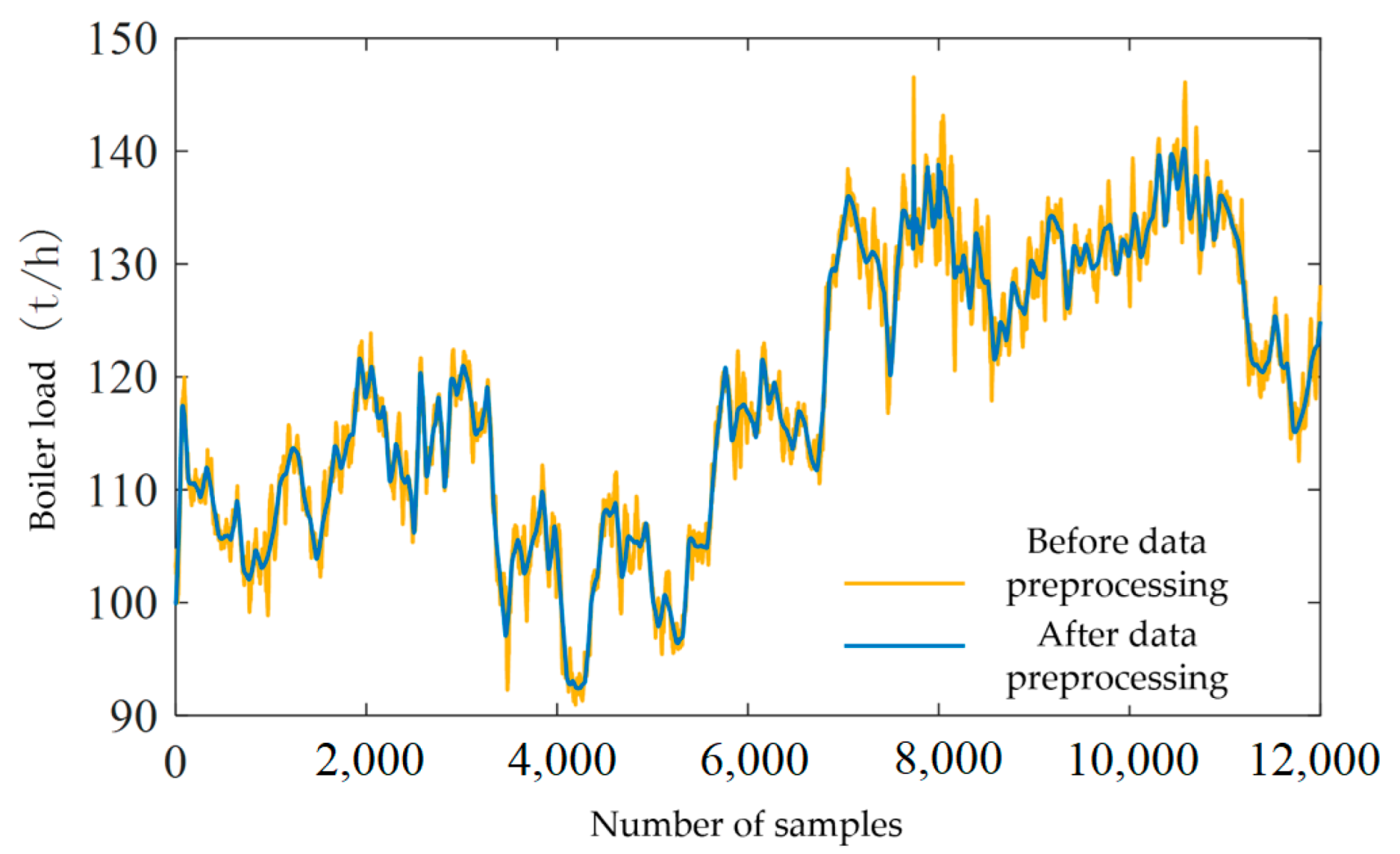
Taking the boiler load of this boiler as an example, Figure 5 shows the results of data pre-processing.

4.2. Model Evaluation Indicators

In order to evaluate the prediction accuracy and generalization performance of the model, the decision coefficient R 2 and the root mean square error R M S E were selected as evaluation indicators, and the evaluation indicators were used for comparing the prediction performance of different models. R 2 and R M S E are defined as follows:
R 2 = y i y ¯ i y ^ i y ^ ¯ i 2 y i y ¯ i 2 y ^ i y ^ ¯ i 2
R M S E = 1 n y i y ^ i 2
where y i , y ¯ i , y ^ i , and y ^ ¯ i , respectively, represent the oxygen content in the flue gas of the sample boiler, the mean of true values, the predicted value, and the mean of predicted values.

4.3. Modeling and Result Analysis

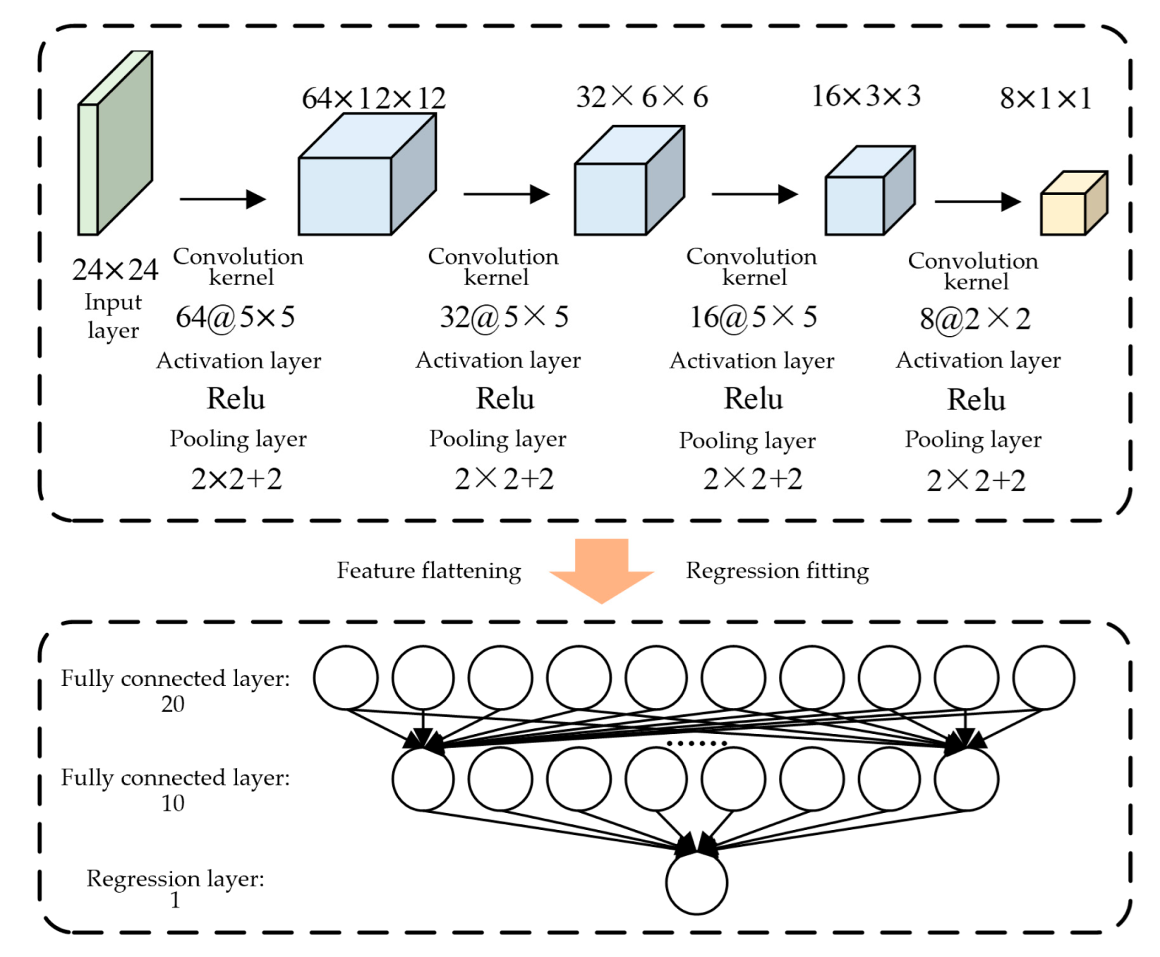
The framework of the prediction model for oxygen content in flue gas based on the CNN is shown in Figure 6, and the hyper-parameter values are shown in Table 3. The hyper-parameters of the TS-CNN model include the maximum number of iterations, the sample size of the minimum training batch, the initial learning rate, the learning rate decline factor, the learning rate decline frequency interval, the discard rate, the optimization algorithm, etc. The optimal values of the hyper-parameters are determined through several experiments as well as empirical values. Cross-validation was performed throughout the test. A total of 80% of the data in the training set were used to create a new training set and the remaining 20% of the data were utilized as a validation set, and each iteration was accompanied by one validation of the model parameters.
The feature extraction module includes four convolution layers, an activation layer, and a pooling layer, respectively. The eight extracted features were flattened and then input into the full connection layer, and there are two full connection layers in total, with 20 and 10 neurons on each layer, respectively, and the last layer is regression layer.
In order to verify the effectiveness of the CNN in the prediction of oxygen content in the flue gas, the following four groups of experiments were designed with different modeling algorithms:
(1)
Time series prediction model (TS-CNN), y n + 1 = f X n ;
(2)
Conventional prediction model (CNN), y n = f X n ;
(3)
BP neural network model (BPNN) with a single hidden layer and 10 neurons;
(4)
Least squares support vector machine model with model parameter γ = 100 ,     σ 2 = 3 (LSSVM).
According to Pearson’s correlation coefficient between variables and oxygen content in the flue gas, boiler load with a correlation coefficient greater than 0.6, lower furnace temperature, furnace outlet temperature, feed water flow, and total feed coal flow were taken as input variables of tests (3) and (4).
The training results of the TS-CNN model and the test results of each model are shown in Figure 7a,b, respectively. It can be seen in Table 4 that the TS-CNN model has the best fitting effect, followed by the CNN model, which indicates that the use of convolution operation for feature extraction of the input matrix can effectively improve the generalization performance of the model. The BPNN model and LSSVM model both have a poor fitting effect, and their prediction curves deviate from the real curves seriously after the 100th test point. The main reasons for the above results are as follows. (1) The boiler has the state accumulation feature, (2) the oxygen content in the boiler flue gas is not only related to other variables but also affected by its own historical change trends, and (3) the feature extraction module in the CNN can extract time sequence features from the input matrix.

5. Conclusions

The boiler system is a complicated nonlinear system with a time lag, where the current value of each operational variable does not accurately describe the current operating state of the boiler, which may be the accumulation of states over a period of time in the past. In order to improve the prediction accuracy of oxygen content in the flue gas, a prediction model for oxygen content in the boiler flue gas based on the CNN was proposed. First of all, the original data were pre-processed using the 3sigam criterion and wavelet denoising. Then, the data were analyzed, and the time series samples in a fixed time window were taken as the input of the model. Additionally, the effect of historical trends of oxygen content in the flue gas on the performance of the model was studied. Considering the boiler flue gas oxygen content may also be affected by its own historical trend, the historical values of the boiler flue gas oxygen content were added to the input of the model for the prediction of the boiler flue gas oxygen content in the next moment. To solve the low efficiency problem of model training caused by too large of a scale of features, a convolution kernel was used to extract the effective features from the input matrix, and a pooling layer was used for dimension reduction in the features. Finally, the TS-CNN model was tested by the actual operating data. The R 2 and R M S E of the TS-CNN model were 0.8929 and 0.1684, respectively, and its prediction accuracy was improved by 18.6%, 31.2%, and 54.6% compared with that of the CNN model, LSSVM model, and BPNN model, respectively. The test results show that the proposed model can effectively predict the oxygen content in the boiler flue gas.
Since all boilers are characterized by complex nonlinearities and time lags, the method proposed in this paper may also be potentially applicable to predict the flue gas oxygen content of a wide range of boilers. In our future research, we will also make an effort to confirm the performance of the proposed method for predicting the flue gas oxygen content of different types of boilers.

Author Contributions

Conceptualization and project administration, B.S.; methodology, Z.L. and G.L.; writing—original draft, Z.L and G.L.; supervision, review, and editing, B.S. All authors have read and agreed to the published version of the manuscript.

Funding

This research was funded by the National Natural Science Foundation of China, funding number 21878238.

Data Availability Statement

The data that support the findings of this study are available from the corresponding author upon reasonable request.

Conflicts of Interest

The authors declare no conflict of interest.

References

  1. Da, B.-W. Strategies for Clean Coal Technologies and Carbon Reduction Investment of Coal-Electric Supply Chain under Cap-and-Trade Model; China University of Mining and Technology: Xuzhou, China, 2021. [Google Scholar]
  2. Liu, C.-L.; Li, S.-N. Soft measurement of flue gas oxygen content based on LS-SVM and simplex. J. Eng. Therm. Energy Power 2010, 25, 292–296. [Google Scholar]
  3. Zhao, C.-Y. Discussion on logic calculation of oxygen content in boiler flue gas for 300MW unit. North China Electr. Power 2007, 8, 12–15. [Google Scholar]
  4. Luo, J.; Wu, L. Research status of soft measurement technology of typical thermal parameters for utility boilers. Therm. Power Gener. 2015, 44, 1–9+13. [Google Scholar]
  5. Liu, F.-G.; Hao, W.-D.; Yang, J.-Z.; Guo, Y.-Q.; Zhang, Q.-G.; Hou, F.-J. Economic analyze for utility boiler operated in different oxygen content outlet furnace and it’s optimization. Proc. CSEE 2003, 23, 172–176. [Google Scholar]
  6. Peng, X.; Lv, Y.-K. Study on analytical solutions on optimal economics of power boiler based on flue gas oxygen content. Electr. Power Sci. Eng. 2009, 25, 40–44. [Google Scholar]
  7. Liang, T.; Jin, Y.-J.; Jiang, W.; Liu, Z.-H. Optimization of NOx emissions from coal-fired boilers based on improved MVO and WLSSVM. China Meas. Test 2021, 47, 148–154. [Google Scholar]
  8. Xie, L.; Mao, G.-M.; Jin, X.-M.; Su, H.-Y. Predictive control and economic performance optimization of CFBB combustion process. CIESC J. 2016, 67, 695–700. [Google Scholar]
  9. Chui, E.-H.; Gao, H. Estimation of NOx emissions from coal-fired utility boilers. Fuel 2010, 89, 2977–2984. [Google Scholar] [CrossRef]
  10. Ma, L.Y.; Wang, Y.; Zuo, X. ANN-based soft sensing of oxygen content in boiler air-flue gas system. In Proceedings of the 2019 Chinese Control and Decision Conference, Nanchang, China, 3–5 June 2019. [Google Scholar]
  11. Zhang, W.; Chen, C.-B.; Wang, J.-C.; Li, J.-C.; Hao, S.-J. Prediction of the oxygen content in flue gas of power plant based on PSO-elman model. Autom. Instrum. 2020, 35, 75–79+85. [Google Scholar]
  12. Geng, M.-Y.; Hu, R.; Li, L. Prediction of oxygen content in boiler flue gas of thermal power unit. J. Univ. Shanghai Sci. Technol. 2021, 43, 319–324+359. [Google Scholar]
  13. Su, T.; Pan, H.-G.; Huang, X.-D.; Shao, X.-Q.; Ma, B. Soft sensor of flue gas oxygen content based on improved PSO-SVM in coal-fired power plant. J. Xi’an Univ. Sci. Technol. 2020, 40, 342–348. [Google Scholar]
  14. Zhang, Y.-F.; Wang, J.-C.; Shi, Y.-H.; Fei, L. Soft sensors model based on state constrained moving window. Control. Eng. China 2014, 21 (Suppl. 1), 115–117+120. [Google Scholar]
  15. Li, J.-Q.; Zhang, Y.-Y.; Niu, C.-L. Prediction of the oxygen content in flue gas of power plant based on PSO-LSSVM model. J. Eng. Therm. Energy Power 2018, 33, 49–55. [Google Scholar] [CrossRef] [Green Version]
  16. Tang, Z.-H.; Chai, X.-Y.; Cao, S.-X.; Mou, Z.-H.; Pang, X.-Y. Deep learning modeling for the NOx emissions of coal-fired boiler considering time-delay characteristics. Proc. CSEE 2020, 40, 6633–6644. [Google Scholar]
  17. Tang, Z.-H.; Li, Y.; Kusiak, A. A deep learning model for measuring oxygen content of boiler flue gas. IEEE Access 2020, 8, 12268–12278. [Google Scholar] [CrossRef]
  18. Tang, Z.-H.; Zhu, D.-Y.; Li, Y. Data driven based dynamic correction prediction model for NOx emission of coal fired boiler. Proc. CSEE 2022, 42, 5182–5193. [Google Scholar]
  19. Li, G.Q.; Qi, X.B.; Chan, K.-C.-C.; Chen, B. Deep bidirectional learning machine for predicting NOx emissions and boiler efficiency from a coal-fired boiler. Energy Fuels 2017, 31, 11471–11480. [Google Scholar] [CrossRef]
  20. Pan, H.; Su, T.; Huang, X.-D.; Wang, Z. LSTM-based soft sensor design for oxygen content of flue gas in coal-fired power plant. Trans. Inst. Meas. Control 2021, 43, 78–87. [Google Scholar] [CrossRef]
  21. Hu, H.-Z.; Zhang, J.-B.; Liu, H.-Q.; Li, M.-D.; Yang, Q.-Y. Power plant boiler combustion efficiency modeling approach based on convolutional neural networks. J. Xi’an Jiaotong Univ. 2019, 53, 10–15. [Google Scholar]
  22. Wang, Z.-Y.; Song, C.-F.; Chen, T. Deep learning based monitoring of furnace combustion state and measurement of heat release rate. Energy 2017, 131, 106–112. [Google Scholar] [CrossRef]
  23. Liu, Y.; Fan, Y.; Chen, J.-H. Flame images for oxygen content prediction of combustion systems using DBN. Energy Fuels 2017, 31, 8776–8783. [Google Scholar] [CrossRef]
  24. Han, Z.-Z.; Li, J.; Zhang, B.; Hossain, M.-M.; Xu, C.-L. Prediction of combustion state through a semi-supervised learning model and flame imaging. Fuel 2020, 289, 119745. [Google Scholar] [CrossRef]
  25. Xing, H.-T.; Guo, J.-L.; Liu, S.-A.; Yan, B.; Yang, Y.-Y. NOx emission forecasting based on CNN-LSTM hybrid neural network. Electron. Meas. Technol. 2022, 45, 98–103. [Google Scholar]
  26. Li, N.; Hu, Y. The deep convolutional neural network for NOx emission prediction of a coal-fired boiler. IEEE Access 2020, 8, 85912–85922. [Google Scholar] [CrossRef]
  27. Jia, X.-J.; Sang, Y.-C.; Li, Y.-J.; Du, W.; Zhang, G.-L. Short-term forecasting for supercharged boiler safety performance based on advanced data-driven modelling framework. Energy 2022, 239, 122449. [Google Scholar] [CrossRef]
Figure 1. Example of the 2D convolution operation.
Processes 11 00990 g001
Figure 2. Example of the multi-channel convolution operation.
Processes 11 00990 g002
Figure 3. Example of max pooling.
Processes 11 00990 g003
Figure 4. The fully connected layer.
Processes 11 00990 g004
Figure 5. The result of data preprocessing.
Processes 11 00990 g005
Figure 6. Framework of the CNN-based model.
Processes 11 00990 g006
Figure 7. (a) Training results of the TS-CNN model. (b) Testing results of different models.
Processes 11 00990 g007
Table 1. Variables of the 130 t/h CFB boiler.
Variable NameUnitScope
Main steam flow ratet/h[90.84, 162.25]
Main steam temperature°C[452.63, 470.31]
Main steam pressureMPa[4.45, 5.04]
Boiler loadt/h[92.40, 140.22]
Drum pressureMPa[4.95, 5.51]
Furnace chamber differential pressurePa[683.05, 1292.18]
Lower furnace temperature°C[854.78, 946.58]
Furnace outlet gas temperature°C[793.60, 919.27]
Furnace outlet air pressurekPa[−607.46, −203.32]
Economizer inlet temperature°C[269.64, 290.63]
Economizer inlet pressurekPa[−2767.96, −1463.91]
Secondary fan outlet temperature°C[4.07, 13.34]
Primary fan outlet temperaturekPa[7.34, 8.46]
Secondary fan outlet pressurekPa[2.64, 5.64]
Feed water pressureMPa[5.36, 6.03]
Feed water temperature°C[149.52, 156.53]
Exhaust outlet temperature°C[123.43, 132.61]
Primary air volumeNm3/h[94,450.76, 102,729.19]
Secondary air volumeNm3/h[69,768.91, 136,108.61]
Feed water flowt/h[85.39, 160.62]
Total coal feed flowt/h[14.09, 23.66]
Current of 1# induced draft fanA[23.86, 32.37]
Current of 2# induced draft fanA[21.84, 33.74]
Oxygen content in boiler flue gas%[3.62, 7.09]
The scope in the above table represents the upper and lower bounds of each variable.
Table 2. Sample example.
VariableUnitSample 1Sample 2Sample 12,000VariableUnitSample 1Sample 2Sample 12,000
Main steam flow ratet/h111.38113.38128.15Primary fan outlet temperaturekPa7.577.588.00
Main steam
temperature
°C464.18464.18464.76Secondary fan outlet pressurekPa3.002.984.50
Main steam
pressure
MPa4.904.884.89Feed water pressureMPa5.625.615.81
Boiler loadt/h103.12103.52128.13Feed water
temperature
°C151.84151.94153.75
Drum pressureMPa5.225.215.37Exhaust outlet
temperature
°C124.88124.91128.18
Furnace chamber differential
pressure
kPa0.750.741.00Primary air volumeNm3/h97,230.7797,406.6094,989.02
Lower furnace temperature°C899.78899.68914.63Secondary air
volume
Nm3/h77,714.2980,263.73108,131.9
Furnace outlet gas temperature°C839.41839.12882.20Feed water flowt/h98.1198.29111.91
Furnace outlet air pressurePa−257.02−255.80−479.24Total coal feed flowt/h15.7315.7819.95
Economizer inlet temperature°C270.70270.70282.42Current of 1#
induced draft fan
A26.4326.5028.37
Economizer inlet pressurekPa−1.589−1.58−2.11Current of 2#
induced draft fan
A21.9421.9626.58
Secondary fan
outlet temperature
°C12.1912.119.21Oxygen content in boiler flue gas%5.575.634.79
Table 3. Parameters for CNN-based model.
Hyper-ParameterNameValue
Maximum number of iterationsMaxEpochs50
Sample size of the minimum training batchminiBatchSize25
Initial learning rateInitialLearnRate0.003
Learning rate decline factorLearnRateDropFactor0.2
Learning rate decline frequency intervalLearnRateDropPeriod8
Discard ratedropout0.2
Optimization algorithmGradient descent with momentum (SGDM)
Table 4. R 2 and R M S E for each model.
TS-CNNCNNBPNNLSSVM
Training set R 2 0.98380.97980.96360.9660
R M S E 0.09030.09860.12830.1240
Test set R 2 0.89290.84430.79630.8251
R M S E 0.16840.20700.37070.2448
Disclaimer/Publisher’s Note: The statements, opinions and data contained in all publications are solely those of the individual author(s) and contributor(s) and not of MDPI and/or the editor(s). MDPI and/or the editor(s) disclaim responsibility for any injury to people or property resulting from any ideas, methods, instructions or products referred to in the content.