Abstract
This study investigates the impact of changes in velocity profiles on the measurement inaccuracies of gas flow streams detected by an ultrasonic flowmeter. The cross-sectional velocity profile was influenced by the downhill flow rate, causing variations in the shape factor coefficient. The flowmeter processing equation should consider the factor of shape coefficient variations. Consideration for these variations can result in errors in the measurement of the flow stream. The processing equation assumes a single, constant value for the shape factor coefficient, which can lead to inaccuracies. This article covers the inaccuracies of the transit-time ultrasonic flowmeter caused by a change in the velocity profile of the flowing gas, such as air. A realistic flow system was established with measured flow rates ranging from 43 m3/h to 225 m3/h. The findings of this study can serve as a valuable reference for the design and implementation of more accurate and efficient flow measurement systems that can enhance process efficiency.
1. Introduction
Flow measurement is essential for precise process control in the engineering field [1,2,3]. Flowmeters employ a range of ways to measure flow, including turbine, orifice, electromagnetic, volumetric, and vortex meters. Nonetheless, the ultrasonic flowmeter (USF) transit-time technique has many advantages [4,5]. When contrasted with conventional membrane gas meters, ultrasonic gas flowmeters exhibit remarkable advantages such as noncontact operation, minimal pressure loss, broad range ratio, and high accuracy [6]. USFs have several applications in the engineering, chemical, and biomedical sectors [7,8]. These devices utilize ultrasonic waves to measure the volumetric flow rate based on the velocity of a fluid moving through a pipe [9]. In the engineering sector, ultrasonic flowmeters are used to monitor water flow in irrigation systems, HVAC systems, and industrial processes [10,11,12]. In the chemical industry, USFs are utilized to measure the flow rate of various chemicals and gases, including corrosive and abrasive substances [13]. Additionally, USFs are also used in the biomedical sector to measure blood flow in veins and arteries, and to monitor the flow rate of liquids in medical devices [14]. Due to their versatility and accuracy, ultrasonic flowmeters have become an essential tool in various industries, providing crucial data for process optimization, equipment maintenance, and quality control [15,16].
Transit-time ultrasonic flowmeters are frequently utilized to perform continuous measurements of medium flow under both steady-state and perturbed conditions [17,18,19,20,21]. Because they are non-contact flow meters, they do not disrupt the flow rate or develop further pressure loss. Their limit error is around +/−2% of the value indicated for the flow stream [22]. High-volume flow rates with high sensitivity can be measured by transmitting ultrasonic frequency between upstream and downstream fixed transducers; liquid velocity can be estimated with 1% accuracy [23]. The installation conditions of the head cap, collection precision, and changes in reference conditions all contribute to inaccuracies in measuring flow streams [24]. Willigen et al. [25] highlighted the challenges faced by ultrasonic flowmeters in measuring fluid flow in industries. The authors presented a new method to minimize zero-flow errors while maintaining a low random error, regardless of the hardware used. The algorithm could adapt to changing zero-flow errors during flow and could combine cross-correlation and zero-crossing detection techniques. Experimental results showed a significant reduction in zero-flow errors without compromising the random error or circuit complexity. The effect of vortices formed in the fluid flow on USF measurements has been investigated [26]. These vortices can cause disturbances in the flow regime, leading to measurement errors in flow rate [27]. To mitigate the effect of vortices on USF measurements, various techniques have been proposed, such as using specialized transducers and signal processing algorithms [28]. Additionally, the location and configuration of the USF in the pipeline can also affect the measurement accuracy [29]. Xuesong [30] conducted a flow field simulation on the pipeline of a mono ultrasonic flowmeter. The flow field characteristics of different shapes and sizes in the pipeline are studied, and the best tapered pipeline model is designed. Studies [20,31] have shown that the positioning of the ultrasonic flowmeters downstream of any obstacles or fittings can minimize the effects of vortices on the measurements. Understanding the effect of vortices on USF measurements is crucial for accurate flow measurement, particularly in applications such as water distribution systems and industrial processes, where vortices are likely to occur. By implementing appropriate techniques and placement of the USF, measurement accuracy can be significantly improved, making it an essential consideration in USF applications [32].
A theoretical design of transit-time USF was performed to improve measurement accuracy [33]. Li et al. [34] presented a novel flow conditioner design for ultrasonic gas flowmeters to enhance measurement accuracy by homogenizing velocity profiles. The effectiveness of the flow conditioner was evaluated using theoretical analysis and numerical simulations, with a 10:1 aspect ratio rectangular fluid channel identified as optimal. A Computational Fluid Dynamics (CFD) model was simulated and validated by an experimental study, showing that the flowmeter with the designed flow conditioner can reduce indication errors by up to 6% and improve repeatability by 0.15%. Nguyen and Park [35] presented a non-invasive ultrasonic flowmeter that utilized a linear array transducer and transmit delay control to vary the incidence angles of ultrasound wave transmission. The flowmeter was evaluated in a specially designed pipe system using the transit-time method with cross-correlation and phase zero-crossing for sub-sample estimation. The proposed multiple angular compensation method with 24 angles was proved to significantly improve the accuracy of measurements up to 93%, compared to invasive electromagnetic measurements with only 74% accuracy. The results suggested that the proposed flowmeter has potential for accurate and non-invasive measurement of the liquid flow in metal pipe systems. Two-phase (gas—liquid) flow measurement models and transit-time were analyzed [36,37,38]. USFs can be used to measure different liquid flows, to operate as autonomous measurement equipment, or as a part of a complex measuring system for automated process control. Energy, attenuation, and noise interference can cause signal fluctuation or even distortion, making it difficult to establish the proper transit time for unstable flow fields. For ultrasonic flowmeters, a peak ratio matching method-based signal processing was proposed [39]. Murakawa et al. [40] highlighted the challenges of accurately measuring steam flow rates in industrial plants using clamp-on time-of-flight ultrasonic flowmeters due to the large acoustic impedance difference between the pipe material and fluid, strong signal attenuation, and high temperature. A new signal processing method was proposed using two ultrasonic transducers to measure the ultrasonic time-of-flight that varied with flow rate. The standard deviation of target signals was proposed for estimating the transit-time difference, which also varied with flow regime and can be used to identify the flow regime. USFs are also used to measure gas flow; an adaptive pulse repetition frequency approach was utilized to measure the transit time of a hot gas flow, and a time-sharing technique was used to run flowmeters concurrently without mutual interference in harsh environmental conditions [41,42]. The measurement accuracy is also affected by changes in the velocity profile of the flowing medium in the pipeline, which relies on the Reynolds number (Re) [43]. Turbulence induced by invading structures in pipes adds uncertainty to measurements, introducing an average relative error for laminar and turbulent flows [44]. A multipath arrangement was employed in implementing gas flow measurement; flowmeter modules, comprising the acoustic path arrangement, ultrasonic emission, and reception module, were constructed systematically [45,46]. Sakhavi and Nouri [47] presented a generalized velocity model for multipath ultrasonic phased array flowmeters. These flowmeters use phased array transducers to electronically sweep ultrasonic beams, reducing the number of transducers required. However, the accuracy of the flow measurement is affected when the flow field deviates from the assumed velocity model. The results showed that the generalized model can reduce the sensitivity of the flowmeters to flow field deviations, with a minimum mean relative error of 1.64% under symmetric and asymmetric flow fields. A recent study by the same authors introduced a multipath ultrasonic flowmeter that utilized phased array transducers and numerical integration [48]. The performance of the flowmeter was studied for different flow fields, and the impact of various factors, such as the number of paths, beam angle, and installation angle, was analyzed. The flowmeter achieved a low relative error of 0.03% under symmetric velocity profiles and a minimum error range of 0.14% under a 5-path arrangement for asymmetric velocity profiles. The validity of the flowmeter was confirmed through computational fluid dynamics simulation, with a maximum absolute relative error of about 3%.
Recently, studies on enhancing USF for gas flow measurements have been conducted by studying non-linearity using the ray tracing approach or the Gaussian beam method [49,50]. Zheng et al. [49] analyzed the non-linearity in gas ultrasonic flowmeter measurements using the ray acoustics theory. The study utilized two-dimensional ray tracing methods and simulations of DN100 and DN500 diametric single path gas ultrasonic flowmeters to propose a corrected model for velocity measurements that improved measurement accuracy by reducing non-linearity. The corrected model reduced measurement errors by up to 4%. Zheng et al. [50] proposed a novel method based on Gaussian beams to analyze the ultrasonic propagation trajectory, propagation time, and sound pressure distribution in gas ultrasonic flowmeters. This method incorporates flow information into the Gaussian beam equation and was verified through simulations and experiments. The errors between the new method and the COMSOL simulation were found to be less than 1%, and the errors between experiments using different ultrasonic transducers were within ±6%. Sakhavi and Nouri [51] used a phased array transducer in multipath ultrasonic flow meters for non-mechanical velocity measurements. The performance of the flowmeter downstream of a single bend was evaluated using Gaussian quadrature integration formulas with different velocity profile models, and CFD simulation modelled the flow field downstream of the bend. The study revealed that the standard deviations of relative errors vary based on the distance from the bend and the model used, with the single bend model exhibiting a higher error rate compared to symmetric models. Chen et al. [52] developed a high-precision USF for gas flow in 2019. In a realistic ultrasonic flowmeter, the flow stream recovery equation includes the shape factor [52]. For laminar flows, this coefficient has a constant value of K = 0.75. In the case of turbulent flows, it is determined by the Reynolds number and the roughness of the pipeline. The profile of the velocity curve in the cross section varies as the flow stream changes, leading to the parabolic shape for laminar flow. Consequently, the value of the shape factor varies, which may result in further measurement inaccuracy.
After surveying the published studies, the influence of shape factor coefficient variations on flow measurement accuracy has received little attention in published studies, which have primarily focused on other factors such as turbulence and vortices. Therefore, the impact of the shape factor variation on flow stream measurement inaccuracy was examined in this study. Furthermore, the effect of the velocity profile variations on the flow stream measurement error measured using a transit-time ultrasonic flowmeter was investigated. The medium that flowed through the system was maintained at a constant temperature and relative humidity. The ultrasonic flowmeter was a Z-shaped ultrasonic wave path meter with sensors installed on the pipeline wall.
2. Airflow Measurement Method
Figure 1 depicts the method for determining the flow rate of a Z-shaped ultrasonic flowmeter of the transit-time type.

Figure 1.
Principle of flow measurement by Z-shaped ultrasonic flow meter Transit—Time types.
Where c is the velocity of an ultrasonic wave in a fluid; w represents the local velocity of the air; L represents the distance traveled by the ultrasonic wave between the UT1 and UT2 sensors; Φ denotes the angle between the velocity components; WMax represents the maximum velocity of the fluid; R denotes the radius of the pipeline; and r represents a radial distance from the center of the pipeline and is bounded by 0 and R (0 ≤ r ≤ R).
The flow rate is determined by measuring the time difference of the ultrasonic wave as it travels from the UT1 sensor to the UT2 sensor and back. On the elementary path of length dL, the time of flight (dt1) of the ultrasonic wave traveling from the UT1 sensor to the UT2 sensor can be expressed:
where c is the ultrasonic wave velocity in the fluid, and w is the fluid velocity. However, the transition time dt2 from sensor direction UT2 to UT1 is:
Using the subsequent relation that:
The difference in ultrasonic wave transit times between the two sensors (Δt) is calculated to be:
where R is pipeline radius.
Equation (4) can be solved by assuming that the velocity of the medium in the cross-section of the pipeline is constant for w << c. Set the velocity to the maximum velocity Wmax and compute the integral to get:
where R is the pipeline radius; and is the difference in time of flight of the ultrasonic wave from the UT1 to UT2 sensor and back for the condition w = Wmax.
The flow rate in a pipeline (m3/s) can be determined using Equation (6) for a constant flow velocity of the medium:
In the second scenario, a particular velocity model is presumed while computing the integral from Equation (4). The Prandtl equation is one of the well-known models of velocity distribution in a pipeline and is often used as follows [53]:
The Reynolds number and pipeline roughness both affect the exponent 1/n. After solving Equation (4), the time difference Δt for the transition of the ultrasonic wave for this model is:
The flow rate equation (m3/s) may also be written as follows:
In comparing formula Equations (6) and (9) for the same t, we obtain:
The profile is defined as K = 2n/(2n + 1) in Equation (10).
It is obvious from Equation (10) that the shape factor of the actual flow rate is dependent on the coefficient n in the Prandtl equation. However, the value shape factor handled into the computational system in a realistic ultrasonic flowmeter is constant, regardless of the Reynolds number. The value of the coefficient n fluctuates as the flow stream rate changes, and the computation system should consider this change in the flow stream rate equation. Otherwise, the change in the velocity profile causes the flow rate measurement to be inaccurate.
3. Determine n Coefficient Value
The equation given by Troskolaski [54] for hydraulically smooth pipes is one way to figure out the value of n coefficient:
Another way to evaluate the n value in reference [55]:
However, in references [56,57], the n coefficient can be calculated regardless of pipe type, as

Table 1.
Dependence of the n coefficient on the Reynolds number.
However, Waluś [58] recommended using the n coefficient derived from the following equation (Equation (14)):
Errors in the K shape coefficient were obtained using the n coefficient determined from Table 1. The shape coefficients of K11, K12, K13, and K14 were calculated using the n coefficient calculated from Equations (11)–(14) are listed in Table 2, respectively. According to Table 1, the Reynolds number changed from 4000 to 428,000.
Table 2.
Values of the K shape coefficient and errors of this coefficient in relation to selected equations for the n coefficient.
Figure 2 depicts the graphs showing the dependency of the n coefficient on the Reynolds number and the K coefficient errors according to Table 2.
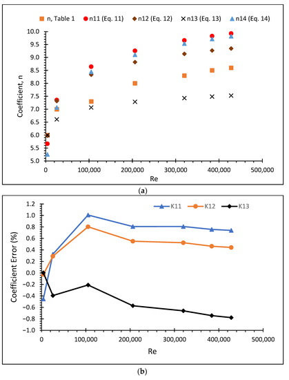
Figure 2.
Relationships of the n coefficient for (a) selected equations and (b) errors of the K shape coefficient in relation to the value of the n coefficient from Table 1.
The calculations demonstrate that the errors associated with the assumption of the K coefficient, regardless of which equation is used, do not exceed 1% when compared to the values in Table 1. They also demonstrate that changing the velocity profile in the Reynolds number range 4000–428,000 and using the n coefficient for any preceding equations, results in a measurement error of less than ±1%.
4. Experimental Procedure
Figure 3 shows the measurements obtained on the stand with an ultrasonic flowmeter of type Prosonics Flow B 200 mounted in a pipeline with an internal diameter dw = 82.6 mm at a distance of approximately 1.8 m behind the elbow. The volume flow rate of the flowing air was computed as the average of 20 measurements obtained directly from the flowmeter display and 20 measurements derived from the current signal reading in the range of (4–20) mA. The airflow was controlled using an inverter in the range of 50 Hz to 10 Hz with a step of 5 Hz to a value of 20 Hz, and then the values of 17 Hz, 15 Hz, 13 Hz, 11 Hz, and 10 Hz were established. The actual volume flow was determined by measuring the volume of 3 m3 of air flowing in time using a turbine gas meter with a maximum range of qvmax = 400 m3/h and an accuracy not exceeding 1% of the observed value. Figure 4 shows a photograph of the installed ultrasonic and turbine flowmeters.

Figure 3.
Real image of measuring system.
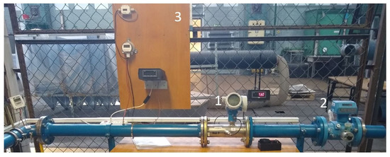
Figure 4.
The measuring system components: (1) ultrasonic flow meter, (2) turbine flow meter, and (3) system for measuring physical parameters of the flowing air.
To ensure the accuracy and reliability of the results obtained from the turbine flowmeter, several measures were taken to minimize measurement errors. Prior to the measurements, the indications of the turbine flowmeter were compared with the values obtained from the measurements of the flows using Proline t-mass F calorimetric flowmeters with a limit error of 1% of the flow rate, vortex type PROWIRL F flowmeters (up to the minimum flow rate that they were capable of measuring) with a limiting error of 1% of the flow rate, and a venturi with a three-disc pressure pickup of the Deltatop type, for several flow streams. The limiting error of the orifice flowmeter was also not greater than 1% of the flow rate. All of these flowmeters were installed in the measurement system.
Furthermore, the turbine flowmeter indications were compared with the results of flow rate measurements performed using a very thin Prandtl tube, which was developed by dividing the cross-section into 6 rings of equal areas. This procedure added an extra layer of assurance to the accuracy and reliability of the results obtained from the turbine flowmeter. Figure 5 shows the vortex and thermal flowmeters installed in the flow system, which were carefully selected for their high accuracy and reliability in measuring flow rates.

Figure 5.
Photos of the: (1) vortex, and (2) thermal flowmeter.
Furthermore, the temperature of the gas was evaluated using a Pt 100 thermometer, and its relative pressure was measured using a magnesense pressure gauge in each measuring cross-section with an accuracy of 1% of the stated value. The calculated flow stream (qv) ranged from 41.87 to 227.28 m3/h.
5. Results and Discussion
The processing equation for the tested ultrasonic flowmeter incorporated both the factor K = 0.933 for n = 7 and an additional factor resulting from the calibration of the flowmeter K* = 1.003. Table 3 summarizes the results of the measurements, displaying the extreme outcomes of the flow stream measurement, i.e., the findings that would be obtained without considering these two factors. This table presents a set of data with various parameters for different values of frequency set on an inverter (F). The other parameters include volume flow measured by an ultrasonic flowmeter (), volume flow measured by a turbine flowmeter (), and volume flow measured by the ultrasonic flowmeter without taking into account the K and K* factors (). The n coefficient value was calculated according to Equation (13). The K** coefficient refers to Equation (15), and the relative error () of the K** factor was evaluated according to Equation (16).
Table 3.
Results of the conducted measurements and calculations.
Figure 6 illustrates how the Reynolds number affects the K** coefficient, whereas Figure 7a shows the relative error of the K** coefficient based on the value of the K coefficient when Equation (13) was utilized to derive the n coefficient values. Figure 7b displays the error of the K** coefficient in relation to the fixed value of the coefficient K = 0.933, which was employed by the manufacturer of the device.
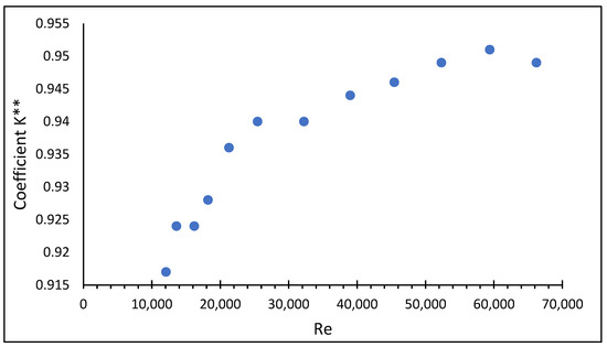
Figure 6.
The values of the K** coefficient versus the Reynolds number.
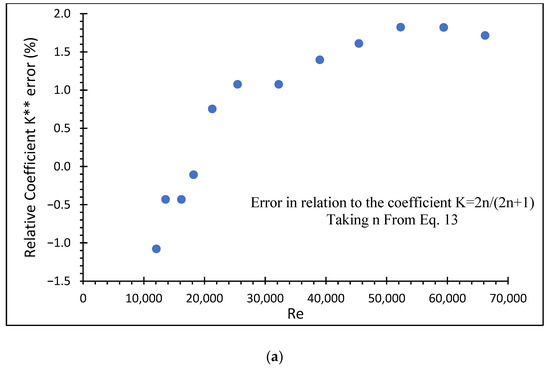

Figure 7.
Relative coefficient K** error (%) versus Reynolds number based on: (a) the value of the K coefficient when Equation (13) was utilized to derive the n coefficient values, and (b) coefficient K = 0.933 according to manufacturer device.
The values of the coefficient n in the studied flow streams range from 6.92 to 6.36, as shown in Table 2. For these n coefficient values, the computed velocity profile shape coefficient K was in the range of K = 0.927–0.933. The percentage difference between the lowest and highest values of the K ratio was 0.64%. As a result, adopting a single, constant value of the aspect ratio in the examined range of Reynolds numbers has little effect on the flow stream measurement inaccuracy. The K** factor comprises all ultrasonic flowmeter adjustments, and its value fluctuated between 0.917–0.949. The relative error of the K shape coefficient ranges from −1.1% to +1.8% compared to the current value of this coefficient. However, compared to the manufacturer’s value of K = 0.933, the relative error of the K** coefficient does not exceed ±2%, as shown in Figure 7. Adopting that the main sources of error are changes in the velocity profile of the flowing gas, even assuming a single, constant value of the K coefficient in the flowmeter processing equation will not result in flow rate errors of more than ±2%. Therefore, in the tested range of the flow streams, the effect of the velocity profile changes associated with the change in the gas flow stream was within the mean limit error of the ultrasonic flowmeter, which was ±2% of the indicated value.
6. Conclusions
This study focuses on the effect of velocity profile variations on the flow stream measurement error measured using a transit-time ultrasonic flowmeter. Measurements were performed at the authors’ initial installation, where the airflow rate was varied from approximately 42 m3/h to 228 m3/h. A turbine flowmeter was used to determine the actual flow rate, which was verified using vortex, thermal, and orifice flowmeters before the measurement. Based on the experimental data, the following conclusions were drawn.
- It can be assumed that the coefficient n, regardless of which equation is used, does not considerably affect the measurement error of the flow stream. For the three selected equations, the error in the K shape coefficient was less than ±1%.
- The correction factor K** was in the range 0.917–0.949, whereas the shape coefficient K ranged from 0.927–0.933. The relative error of the correction factor K** ranged from −1.1% to +1.8%.
- The calculated error value of the correction factor K** for the constant value adopted by the manufacturer, which is equal to K = 0.933, does not exceed the value of ±2%.
- The change in the velocity profile of the air flowing in the installation due to the cold flow stream results in a measurement error of no more than ±2% of the indicated value of the flowmeter, which is within its limit error.
In future studies, the impact of velocity profile changes on flow measurement accuracy in other types of flowmeters, such as Coriolis and electromagnetic flowmeters, will be thoroughly investigated. The effects of fluid viscosity, temperature, and pressure on the accuracy of flow measurement using ultrasonic flowmeters will also be studied in depth. Additionally, more advanced algorithms will be developed to process ultrasonic flowmeter data and account for variations in velocity profile, which could potentially enhance flow measurement accuracy and increase the reliability of ultrasonic flowmeters in various applications. Moreover, the feasibility of using multiple ultrasonic flowmeters to measure the flow in complex systems with varying cross-sectional areas or flow regimes will be explored, aiming to improve flow measurement accuracy in such systems.
Author Contributions
Conceptualization, P.P., W.W., A.A. (Artur Andruszkiewicz) and P.K.; methodology, P.P., W.W., A.A. (Artur Andruszkiewicz) and P.K.; validation, A.A. (Ali Alahmer) and W.W.; formal analysis, S.A. (Sameh Alsaqoor), P.P., A.A. (Ali Alahmer), S.A. (Samer As’ad) and A.A. (Artur Andruszkiewicz); investigation, S.A. (Sameh Alsaqoor), P.P., A.A. (Ali Alahmer), W.W. and P.K.; resources, P.P., W.W., A.A. (Artur Andruszkiewicz) and P.K.; writing—original draft preparation, S.A. (Sameh Alsaqoor), P.P., A.A. (Ali Alahmer) and N.B.; writing—review and editing, A.A. (Ali Alahmer) and A.A. (Artur Andruszkiewicz); visualization, A.A. (Ali Alahmer), S.A. (Samer As’ad) and N.B.; funding, S.A. (Samer As’ad). All authors have read and agreed to the published version of the manuscript.
Funding
This research received no external funding.
Data Availability Statement
Not available.
Acknowledgments
The authors express their gratitude to the Middle East University in Amman, Jordan for providing financial support to cover the publication fees associated with this research article.
Conflicts of Interest
The authors declare no conflict of interest.
References
- Ferrari, A.; Pizzo, P.; Rundo, M. Modelling and Experimental Studies on a Proportional Valve Using an Innovative Dynamic Flow-Rate Measurement in Fluid Power Systems. Proc. Inst. Mech. Eng. Part C J. Mech. Eng. Sci. 2018, 232, 2404–2418. [Google Scholar] [CrossRef]
- Mohammed, S.; Abdulkareem, L.; Roshani, G.H.; Eftekhari-Zadeh, E.; Haso, E. Enhanced Multiphase Flow Measurement Using Dual Non-Intrusive Techniques and ANN Model for Void Fraction Determination. Processes 2022, 10, 2371. [Google Scholar] [CrossRef]
- Aljabarin, N.; Al-Amayreh, M.; Alahmer, A.; Alsaqoor, S. Experimental Determination of a Minimum Spouting Velocity for Ceramic-Coated Bearings in Conical-Cylindrical Spouted Beds. J. Porous Media 2022, 25, 1–13. [Google Scholar] [CrossRef]
- Lynnworth, L.C.; Liu, Y. Ultrasonic Flowmeters: Half-Century Progress Report, 1955–2005. Ultrasonics 2006, 44, e1371–e1378. [Google Scholar] [CrossRef] [PubMed]
- Qiu, Y.; Chen, H.; Li, W.; Wu, F.; Li, Z. Optimization of the Tracer Particle Addition Method for PIV Flowmeters. Processes 2021, 9, 1614. [Google Scholar] [CrossRef]
- Fonseca, G.E.; Dube, M.A.; Penlidis, A. A Critical Overview of Sensors for Monitoring Polymerizations. Macromol. React. Eng. 2009, 3, 327–373. [Google Scholar] [CrossRef]
- Güler, I.; Güler, N.F. Precision of the Time-Domain Correlation Ultrasonic Flowmeter. Med. Biol. Eng. Comput. 1991, 29, 447–450. [Google Scholar] [CrossRef]
- Awad, A.S.; Abulghanam, Z.; Fayyad, S.M.; Alsaqoor, S.; Alahmer, A.; Aljabarin, N.; Piechota, P.; Andruszkiewicz, A.; Wędrychowicz, W.; Synowiec, P. Measuring the Fluid Flow Velocity and Its Uncertainty Using Monte Carlo Method and Ultrasonic Technique. Wseas Trans. Fluid Mech. 2020, 15, 172–182. [Google Scholar] [CrossRef]
- Schulenberg, T.; Stieglitz, R. Flow Measurement Techniques in Heavy Liquid Metals. Nucl. Eng. Des. 2010, 240, 2077–2087. [Google Scholar] [CrossRef]
- Abu-Mahfouz, I. Flow Rate Measurements. In Instrumentation: Theory and Practice Part II: Sensors and Transducers; Springer: Berlin/Heidelberg, Germany, 2022; pp. 77–102. [Google Scholar]
- Doyle, F.; Duarte, M.-J.R.; Cosgrove, J. Design of an Embedded Sensor Network for Application in Energy Monitoring of Commercial and Industrial Facilities. Energy Procedia 2015, 83, 504–514. [Google Scholar] [CrossRef]
- AlSaqoor, S.; Alahmer, A.; Al Quran, F.; Andruszkiewicz, A.; Kubas, K.; Regucki, P.; Wędrychowicz, W. Numerical Modeling for the Retrofit of the Hydraulic Cooling Subsystems in Operating Power Plant. Therm. Eng. 2017, 64, 551–558. [Google Scholar] [CrossRef]
- Irshad, H.M.; Toor, I.U.; Badr, H.M.; Samad, M.A. Evaluating the Flow Accelerated Corrosion and Erosion–Corrosion Behavior of a Pipeline Grade Carbon Steel (AISI 1030) for Sustainable Operations. Sustainability 2022, 14, 4819. [Google Scholar] [CrossRef]
- Yáñez, C.; DeMas-Giménez, G.; Royo, S. Overview of Biofluids and Flow Sensing Techniques Applied in Clinical Practice. Sensors 2022, 22, 6836. [Google Scholar] [CrossRef] [PubMed]
- Fonseca, V.D.; Duarte, W.M.; de Oliveira, R.N.; Machado, L.; Maia, A.A.T. Mass Flow Prediction in a Refrigeration Machine Using Artificial Neural Networks. Appl. Therm. Eng. 2022, 214, 118893. [Google Scholar] [CrossRef]
- Javaid, M.; Haleem, A.; Singh, R.P.; Rab, S.; Suman, R. Significance of Sensors for Industry 4.0: Roles, Capabilities, and Applications. Sens. Int. 2021, 2, 100110. [Google Scholar] [CrossRef]
- Ma, L.; Liu, J.; Wang, J. Study of the Accuracy of Ultrasonic Flowmeters for Liquid. AASRI Procedia 2012, 3, 14–20. [Google Scholar] [CrossRef]
- Synowiec, P.; Andruszkiewicz, A.; Wędrychowicz, W.; Piechota, P.; Wróblewska, E. Influence of Flow Disturbances behind the 90° Bend on the Indications of the Ultrasonic Flow Meter with Clamp-On Sensors on Pipelines. Sensors 2021, 21, 868. [Google Scholar] [CrossRef]
- Papathanasiou, P.; Kissling, B.; Berberig, O.; Kumar, V.; Rohner, A.; Bezděk, M. Flow Disturbance Compensation Calculated with Flow Simulations for Ultrasonic Clamp-on Flowmeters with Optimized Path Arrangement. Flow Meas. Instrum. 2022, 85, 102167. [Google Scholar] [CrossRef]
- Alsaqoor, S.; Alahmer, A.; Andruszkiewicz, A.; Piechota, P.; Synowiec, P.; Beithu, N.; Wędrychowicz, W.; Wróblewska, E.; Jouhara, H. Ultrasonic Technique for Measuring the Mean Flow Velocity behind a Throttle: A Metrological Analysis. Therm. Sci. Eng. Prog. 2022, 34, 101402. [Google Scholar] [CrossRef]
- Mahadeva, D.V.; Baker, R.C.; Woodhouse, J. Further Studies of the Accuracy of Clamp-on Transit-Time Ultrasonic Flowmeters for Liquids. IEEE Trans. Instrum. Meas. 2009, 58, 1602–1609. [Google Scholar] [CrossRef]
- Brassier, P.; Hosten, B.; Vulovic, F. High-Frequency Transducers and Correlation Method to Enhance Ultrasonic Gas Flow Metering. Flow Meas. Instrum. 2001, 12, 201–211. [Google Scholar] [CrossRef]
- Swengel, R.C.; Hess, W.B.; Waldorf, S.K. Demonstration of the Principles of the Ultrasonic Flowmeter. Electr. Eng. 1954, 73, 1082–1084. [Google Scholar] [CrossRef]
- Waluś, S. Przepływomierze Ultradźwiękowe: Metodyka Stosowania; Wydawnictwo Politechniki Śląskiej: Gliwice, Poland, 1997; ISBN 8385718435. [Google Scholar]
- van Willigen, D.M.; van Neer, P.L.M.J.; Massaad, J.; de Jong, N.; Verweij, M.D.; Pertijs, M.A.P. An Algorithm to Minimize the Zero-Flow Error in Transit-Time Ultrasonic Flowmeters. IEEE Trans. Instrum. Meas. 2020, 70, 1–9. [Google Scholar] [CrossRef]
- Lo̸land, T.; Sætran, L.R.; Olsen, R.; Gran, I.R.; Sakariassen, R. Fluid Motion in Ultrasonic Flowmeter Cavities. J. Fluids Eng. 1999, 12, 422–426. [Google Scholar] [CrossRef]
- Geoghegan, P.H.; Buchmann, N.A.; Soria, J.; Jermy, M.C. Time-Resolved PIV Measurements of the Flow Field in a Stenosed, Compliant Arterial Model. Exp. Fluids 2013, 54, 1528. [Google Scholar] [CrossRef]
- Ren, R.; Wang, H.; Sun, X.; Quan, H. Design and Implementation of an Ultrasonic Flowmeter Based on the Cross-Correlation Method. Sensors 2022, 22, 7470. [Google Scholar] [CrossRef] [PubMed]
- Mousavi, S.F.; Hashemabadi, S.H.; Jamali, J. Calculation of Geometric Flow Profile Correction Factor for Ultrasonic Flow Meter Using Semi-3D Simulation Technique. Ultrasonics 2020, 106, 106165. [Google Scholar] [CrossRef] [PubMed]
- Zhao, X. Development of Single-Path Ultrasonic Flowmeter. Master’s Thesis, China Jiliang University, Hangzhou, China, 2013. [Google Scholar]
- Martins, R.S.; Andrade, J.R.; Ramos, R. On the Effect of the Mounting Angle on Single-Path Transit-Time Ultrasonic Flow Measurement of Flare Gas: A Numerical Analysis. J. Braz. Soc. Mech. Sci. Eng. 2020, 42, 13. [Google Scholar] [CrossRef]
- Webster, J.G.; Eren, H. Measurement, Instrumentation, and Sensors Handbook: Two-Volume Set; CRC Press: Boca Raton, FL, USA, 2018; ISBN 1439863261. [Google Scholar]
- Chen, G.; Liu, G.; Zhu, B.; Tan, W. 3D Isosceles Triangular Ultrasonic Path of Transit-Time Ultrasonic Flowmeter: Theoretical Design and CFD Simulations. IEEE Sens. J. 2015, 15, 4733–4742. [Google Scholar] [CrossRef]
- Li, L.; Zheng, X.; Gao, Y.; Hu, Z.; Zhao, J.; Tian, S.; Wu, Y.; Qiao, Y. Experimental and Numerical Analysis of a Novel Flow Conditioner for Accuracy Improvement of Ultrasonic Gas Flowmeters. IEEE Sens. J. 2022, 22, 4197–4206. [Google Scholar] [CrossRef]
- Nguyen, T.H.L.; Park, S. Multi-Angle Liquid Flow Measurement Using Ultrasonic Linear Array Transducer. Sensors 2020, 20, 388. [Google Scholar] [CrossRef] [PubMed]
- Xing, L.; Hua, C.; Zhu, H.; Drahm, W. Flow Measurement Model of Ultrasonic Flowmeter for Gas-Liquid Two-Phase Stratified and Annular Flows. Adv. Mech. Eng. 2014, 6, 194871. [Google Scholar] [CrossRef]
- Simurda, M.; Lassen, B.; Duggen, L.; Basse, N.T. A Fourier Collocation Approach for Transit-Time Ultrasonic Flowmeter under Multi-Phase Flow Conditions. J. Comput. Acoust. 2017, 25, 1750005. [Google Scholar] [CrossRef]
- Synowiec, P.; Andruszkiewicz, A.; Wędrychowicz, W.; Regucki, P. Research on the Possibility of Measuring the Flow Rate of a Two-Phase Medium with an Ultrasonic Flowmeter. J. Przegląd Elektrotechniczny 2015, 10, 179–182. [Google Scholar]
- Chen, J.; Chen, S.; Li, B.; Lu, J. Research on a Transit-Time Liquid Ultrasonic Flowmeter under Unstable Flow Fields. Meas. Sci. Technol. 2019, 30, 55902. [Google Scholar] [CrossRef]
- Murakawa, H.; Ichimura, S.; Sugimoto, K.; Asano, H.; Umezawa, S.; Sugita, K. Evaluation Method of Transit Time Difference for Clamp-on Ultrasonic Flowmeters in Two-Phase Flows. Exp. Therm. Fluid Sci. 2020, 112, 109957. [Google Scholar] [CrossRef]
- Kupnik, M.; Schroder, A.; O’Leary, P.; Benes, E.; Groschl, M. Adaptive Pulse Repetition Frequency Technique for an Ultrasonic Transit-Time Gas Flowmeter for Hot Pulsating Gases. IEEE Sens. J. 2006, 6, 906–915. [Google Scholar] [CrossRef]
- Kupnik, M.; Gröschl, M. Ultrasonic-Based Gas Flowmeter for Harsh Environmental Conditions. e&i Elektrotechnik Informationstechnik 2009, 126, 206–213. [Google Scholar]
- Zhang, H.; Guo, C.; Lin, J. Effects of Velocity Profiles on Measuring Accuracy of Transit-Time Ultrasonic Flowmeter. Appl. Sci. 2019, 9, 1648. [Google Scholar] [CrossRef]
- Jie, G.; Dong, L.; Guang-Sheng, D.; Zheng-Gang, L.; De-Cai, H. Detection of Turbulent Error by Helicity in an Ultrasonic Flowmeter. Trans. Inst. Meas. Control 2019, 41, 1110–1122. [Google Scholar] [CrossRef]
- Chen, Q.; Li, W.; Wu, J. Realization of a Multipath Ultrasonic Gas Flowmeter Based on Transit-Time Technique. Ultrasonics 2014, 54, 285–290. [Google Scholar] [CrossRef] [PubMed]
- Kurniadi, D. Transit Time Multipath Ultrasonic Flowmeter: An Issue on Acoustic Path Arrangement. In Applied Mechanics and Materials; Trans Tech Publications Ltd.: Zurich, Switzerland, 2015; Volume 771, pp. 3–8. [Google Scholar]
- Sakhavi, N.; Nouri, N.M. Generalized Velocity Profile Evaluation of Multipath Ultrasonic Phased Array Flowmeter. Measurement 2022, 187, 110302. [Google Scholar] [CrossRef]
- Nouri, N.M.; Sakhavi, N. Numerical Analysis of Liquid Flow Measurement Using Multipath Ultrasonic Phased Array Flowmeter. Ultrasonics 2023, 128, 106859. [Google Scholar] [CrossRef]
- Zheng, D.; Mei, J.; Wang, M. Improvement of Gas Ultrasonic Flowmeter Measurement Non-linearity Based on Ray Tracing Method. IET Sci. Meas. Technol. 2016, 10, 602–606. [Google Scholar] [CrossRef]
- Zheng, D.; Lv, S.-H.; Mao, Y. A New Method for Researching the Acoustic Field of a Gas Ultrasonic Flowmeter Based on a Gaussian Beam. Meas. Sci. Technol. 2019, 30, 45004. [Google Scholar] [CrossRef]
- Sakhavi, N.; Nouri, N.M. Performance of Novel Multipath Ultrasonic Phased Array Flowmeter Using Gaussian Quadrature Integration. Appl. Acoust. 2022, 199, 109004. [Google Scholar] [CrossRef]
- Chen, J.; Zhang, K.; Wang, L.; Yang, M. Design of a High Precision Ultrasonic Gas Flowmeter. Sensors 2020, 20, 4804. [Google Scholar] [CrossRef] [PubMed]
- White, F.M.; Majdalani, J. Viscous Fluid Flow; McGraw-Hill: New York, NY, USA, 2006. [Google Scholar]
- Troskolański, A.T. Hydromechanika Techniczna: Hydraulika; Państwowe Wydawn Techniczne: Warszawa, Poland, 1954. [Google Scholar]
- Miller, R.W. Flow Measurement Engineering Handbook; Instrument Society of America: Research Triangle Park, NC, USA, 1983. [Google Scholar]
- Spitzer, D.W. Industrial Flow Measurement; Instrument Society of America: Research Triangle Park, NC, USA, 1984. [Google Scholar]
- Kegel, T.M. Insertion (Sampling) Flow Measurement. In Flow Measurement; Instrument Society of America: Research Triangle Park, NC, USA, 1991. [Google Scholar]
- Waluś, S. Optymalizacja Metrologiczna Pomiaru Strumienia Płynu za Pomocą Przepływomierzy Próbkujących; Wydawnictwo Politechniki Śląskiej: Gliwice, Poland, 2003; ISBN 8373351043. [Google Scholar]


Disclaimer/Publisher’s Note: The statements, opinions and data contained in all publications are solely those of the individual author(s) and contributor(s) and not of MDPI and/or the editor(s). MDPI and/or the editor(s) disclaim responsibility for any injury to people or property resulting from any ideas, methods, instructions or products referred to in the content. |
© 2023 by the authors. Licensee MDPI, Basel, Switzerland. This article is an open access article distributed under the terms and conditions of the Creative Commons Attribution (CC BY) license (https://creativecommons.org/licenses/by/4.0/).