Article

Multi-Period Production Optimization Decision Models under Net-Zero Transformation

Department of Business Administration, National Central University, Jhongli, Taoyuan 32001, Taiwan
Processes 2023, 11(5), 1439; https://doi.org/10.3390/pr11051439
Submission received: 29 March 2023 / Revised: 26 April 2023 / Accepted: 29 April 2023 / Published: 9 May 2023
(This article belongs to the Topic Multiple Roads to Achieve Net-Zero Emissions by 2050)

Abstract

:
Facing the goal of net-zero emissions in 2050, the EU will pilot the European Carbon Boundary Adjustment Mechanism (CBAM) in 2023 and formally implement it in 2026. The scope of control includes cement, electricity, fertilizer, steel, aluminum, and five high-carbon emission industries. In response to global net-zero emissions and CBAM trends, net-zero transformation is not only an environmental issue but also a major economic issue related to Taiwan’s aluminum wheel frame industry. This study aims to bridge this gap by developing novel decision-making models that consider the unique requirements and constraints of net-zero transition, leading to more efficient and sustainable production optimization strategies based on activity-based costing (ABC). This study proposes four possible multi-period production optimization decision-making models (carbon tax and credit combination models) under the net-zero emission transformation of the aluminum wheel frame industry, and it compares the models to test their differences. The results of the study point out that, due to the different roles of carbon tax and carbon credit, the profit and product structure under the net-zero transformation will be very different. Enterprises should formulate carbon emission reduction targets and carbon inventories as soon as possible.

1. Introduction

According to data released by the United Nations Intergovernmental Panel on Climate Change (IPCC) at the end of October 2022, the global average temperature will have increased by 1.1 °C by 2021 compared with before the Industrial Revolution. The parties to the United Nations Framework Convention on Climate Change pledged in November 2021 to halve carbon emissions by 2030, and to achieve net zero by 2050 at the latest, in order to achieve this century’s target increase in temperature within 1.5 °C. Governments and businesses around the world are looking for possible solutions to help maintain the environment [1,2,3]. According to the 2018 Greenhouse Gas Emissions List released by the Environmental Protection Agency of the Executive Yuan in Taiwan, among all industries, the second highest industry is the industrial process sector in addition to the general energy consumption sector. Facing the goal of net-zero emissions in 2050, the European Union will implement the European Carbon Border Adjustment Mechanism (CBAM) on a trial basis in 2023 and implement it formally in 2026. The CBAM will set a carbon price based on the average price of carbon trading in the EU Emissions Trading System (EU ETS). Imported products in the EU need to pay the same carbon cost as their domestically produced goods and use CBAM vouchers to offset imported carbon emissions. If the carbon emission cost of the manufacturer has paid the carbon price in the production country and can issue a complete certificate, the relevant costs can be offset when importing into the EU [4,5,6,7,8]. This system must rely on the close cooperation between the government and enterprises to reduce environmental damage. The company’s most direct method is to reduce the total carbon emissions in the entire production process by comparing the costs and profits of different production models and measuring the carbon tax and carbon trading settings [9]. The control scope includes cement, electricity, fertilizer, steel, aluminum, and five high-carbon emission industries. Therefore, this article takes the production cost planning model of the aluminum rim industry as an example to discuss net-zero transformation.
In response to the global net-zero emissions and CBAM trends, net-zero transformation is not only an environmental issue, but also a major economic issue related to Taiwan’s aluminum wheel frame industry. The purpose of this article is to propose a production planning and control framework under Industry 4.0, taking the aluminum wheel industry as an example [10,11]. As shown in Figure 1. The main focus is on designing different production cost models, matching different carbon tax cost equations and carbon rights trading mechanisms to find the best solution for the product process, and to simulate the product sales and production quantities for enterprises to maximize profits and cost consumption. Through activity-based costing (ABC), enterprise costs are accurately estimated, and system constraints are identified and managed through Theory of Constraints (TOC). Production managers can learn about the best combination of products through the production planning section and seek the greatest profit [12]. Obtaining the highest profit at the lowest cost is always the main goal pursued by all companies. One of the well-known methods to solve the cost problem is activity-based costing, which examines each operation to determine the most accurate cost for each product [12,13]. This study uses the basic model of Tsai, W.-H., and Chu, P.-Y. (2019) for further analysis [11]. Ruidas’ (2022) study discusses four different policies (simple tax policy, cap and buy policy, cap and incentive policy, and strictly permitted cap policy) and develops four different inventory models based on these policies [14]. The features of the current research compared to other ones with a focus on solving production optimization decision are shown in Table 1. The paper proposes five models under Industry 4.0. The cost of carbon tax and the carbon trading function are the second and fourth models. This article further analyzes the impact of different carbon taxes and carbon trading models on profits. The contribution of this article is to enable the government and enterprises to understand all the possible situations of carbon tax and carbon rights well [15]. Therefore, four models are proposed in this article: the carbon tax model with an incremental tax rate without allowance, an incremental tax rate without allowance and the carbon trading model, the carbon tax model with an incremental tax rate with allowances, and an incremental tax rate with allowances and the carbon trading model. This article also compares each model to help companies understand the possible situation well after the policy is announced, and to make it easier for the government to understand the impact that each policy may have on the company.
The rest of this article is arranged as follows. The background of this study is described in Section 2. The green production planning model under the four kinds of activity-based costing methods is depicted in Section 3. Section 4 is the internal data of the aluminum wheel industry sample company. These data are the basic parameters of the model in Section 3. Section 4 also compares and analyzes each model. Finally, Section 5 proposes a brief discussion and conclusion.

2. Research Background

In all industries, “green” is the main trend. Green products are safer for people and the planet and contain varying degrees of reusability, thereby saving costs. The concept of “green enterprise” makes people consider the purpose of the company’s existence [17] and how to coexist with the environment. In the past, the goal of enterprises was to maximize economic profits or improve customer service [18], but now the environmental theme plays a very important role, becoming the central point of strategy and operational management policies. Whether it is nickel-aluminum bronze, manganese bronze, or any of the two, green alloys are environmentally friendly metal alloys with extremely low lead content, and in some cases even no lead at all. Usually, they do not contain elements known to be harmful to the environment or humans and animals, and they are usually made from recycled ingredients. The Das, SK, Green, JAS, and Kaufman, JG (2007) study showed that the use of aluminum alloys in transportation continued to increase and stated the economic benefits of recycling vehicles rich in aluminum [19]. Ruidas’ (2021) study mainly explored the effect of joint investment in green innovation and the impact of emission reduction technology on the green production inventory model [16]. When recycling several aluminum recycling practices and systems for passenger cars, the possible components have been determined, and the use of direct recycling has been preliminary evaluated, and the specific components of possible new recyclable alloys have been suggested.
The net-zero transformation of the aluminum-alloy wheel frame industry refers to achieving carbon neutrality by reducing emissions. In terms of ESG (environment, society, governance), the impact on the environment can be reduced by reducing energy and resource consumption, for example by using renewable energy, recycling and reusing materials, etc. In addition, the industry should take steps to reduce emissions, for example by using clean energy, and implement programs to reduce waste and reduce chemical use. The aluminum wheel industry is expected to respect the rights and benefits of employees and ensure their safety and health in the workplace. In addition, the industry should ensure that its governance structures are sound and ensure compliance with laws and regulations and sustainability strategies and goals through transparent and accountable management practices to achieve net-zero transformation. In conclusion, the performance of the aluminum-alloy wheel frame industry in terms of ESG and net-zero transformation are key factors to achieve sustainable development, and companies need to take active measures to achieve it. The Aluminum Association proposed that aluminum has a long service life in its report (Aluminum: The Element of Sustainability) on the elements of sustainable aluminum development, and it involves many stakeholders at every stage of its life, which makes the sustainability of the cycle of managing life in an efficient manner become a challenge [20]. It is usually not feasible to track the fate of individual metals with long usage times, multiple ownership changes, and highly variable scrap recovery and recycling methods [21]. The study by Sarkar (2022) investigated variable production systems with substitute products under the influence of carbon emissions and green technologies [22]. Luo (2022) developed four game-theoretic models to assess the impact of carbon tax policies on manufacturing and remanufacturing decisions in a closed-loop supply chain (CLSC) consisting of manufacturers and retailers [23]. In order to make quantifiable progress in sustainability management, science must strive to develop appropriate methods to understand the exact level of material loss at the end of life and the cause of the loss. Scientists have developed many methods for understanding product recycling, including statistical surveys and system construction. In the face of rapid global population growth in the 21st century, natural population reduction in resources and environmental degradation, the aluminum industry must do more to guide society to expand and deepen the use of aluminum in order to achieve sustainable development solutions. This may include incorporating factors such as emission reduction technologies and sustainability considerations into the decision-making process.
The following introduces two methods commonly used in the mathematical programming model of this paper. Activity-based costing (ABC) is a method to help companies effectively estimate production and environmental costs [24,25]. This method measures the cost of related activities through all the resources used to manufacture the product. This method can also trace these related costs back to cost centers or departments [26,27,28]. Companies can effectively choose product combinations to reduce production costs and increase profits. However, in addition to using the ABC method, the product portfolio also incorporates the Theory of Constraints (TOC) [29]. The TOC is a method to achieve the optimal allocation of resources and can help enterprises to perform short-term optimization procedures [15]. The TOC theory is not only applicable to manufacturing to find the best production volume, but also to project management. It is a process of continual optimization of the system and continuous improvement by identifying the limitations of the system to find out the reasons that affect the progress of the project [30]. The existing literature may lack a holistic approach that adequately addresses the complexities and challenges associated with transitioning to a net-zero carbon economy in the context of production optimization decision models. Therefore, this study aims to bridge this gap by developing novel decision-making models that consider the unique requirements and constraints of net-zero transition, leading to more efficient and sustainable production optimization strategies.

3. Research Model

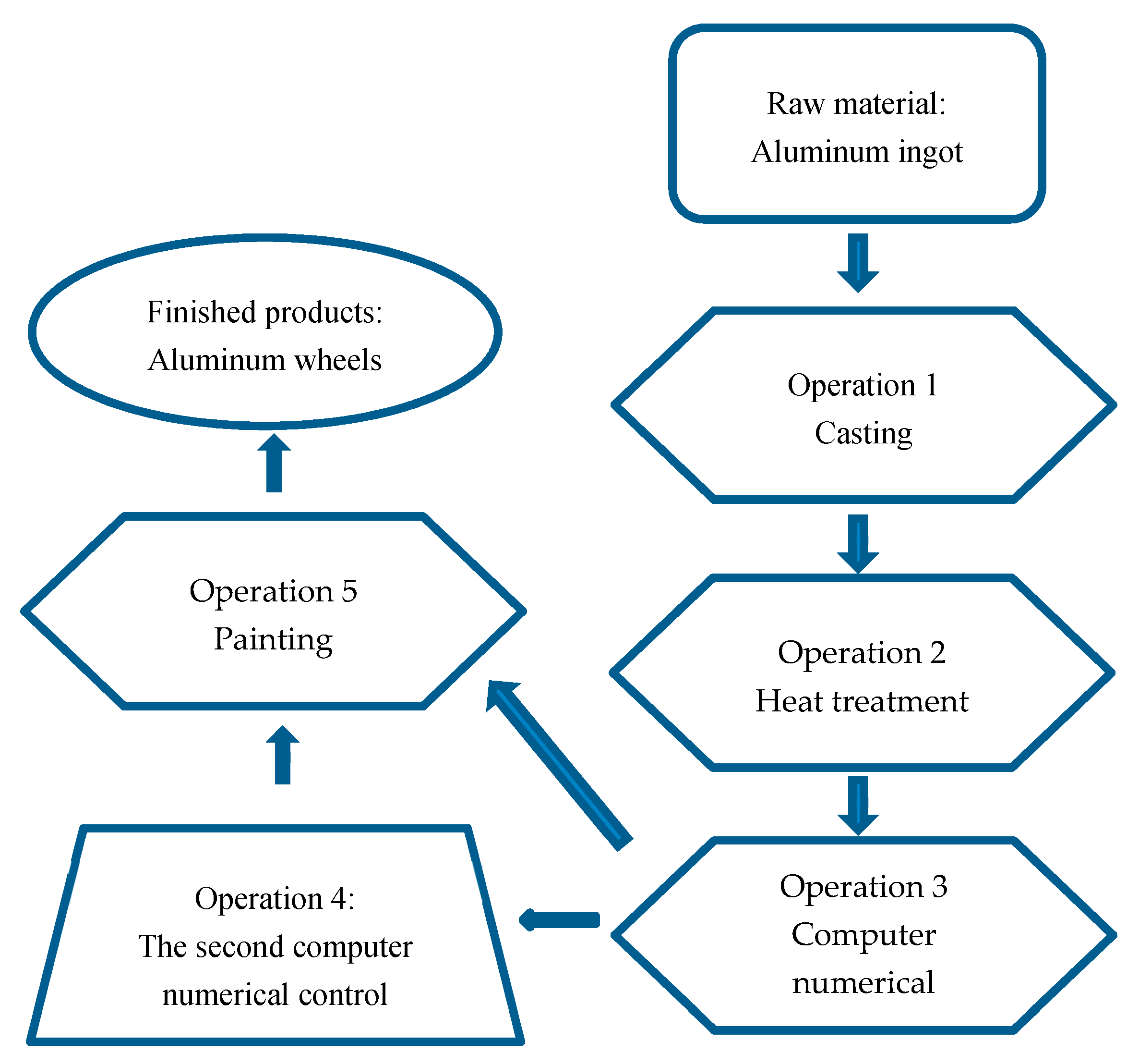
In this study, aluminum rim companies are used as an example. The common production process of aluminum rims can be simplified into four main steps, as shown in Figure 2. The production process includes casting (o = 1), heat treatment (o = 2), computer numerical control (CNC) (o = 3, 4), and painting (o = 5). The second step of CNC machining is an optional process and is only used for certain products that require a second machining for enhanced functionality. Basically, when changing from a single period to a multi-period, the unknown variables are assumed to be different in each period, and the variable symbols in the mathematical programming mode are added with the subscript t representing the time. In terms of known parameters, under all assumptions, only the parameters that are different in each period need to be added with the subscript t representing the time in the parameter symbols of the mathematical programming mode. This section extends the model of the previous research for illustration, including the multi-phase model of two models. Section 3.1 discusses the basic production model and Section 3.2 and Section 3.3 only list the multi-phase models of carbon tax costs and consider two other conditions: (1) In the multi-period situation, when carbon emission allowances or carbon rights can be stored or borrowed, the production decisions and total profits of each model are impacted; (2) In the case of multiple periods, the material requirement quantity specifies the upper limit quantity in the total period, which affects the production decision and profit of each model.

3.1. Multi-Phase Model of the Basic Production Model

3.1.1. Objective Function

The production process includes casting (o = 1), heat treatment (o = 2), computer numerical control (CNC) (o = 3, 4), and painting (o = 5). The second step of CNC machining is an optional process and is only used for certain products that require a second machining for enhanced functionality. Direct material discounts are very common in the current commercial situation. When the buyer or customer has greater power to bargain with the seller or supplier, or the seller or supplier is willing to negotiate with the buyer as a long-term company partner or negotiate with the buyer, direct labor usually refers to the human resources used in the production line. The third group of formulas in Equation (1), H R 1 + ω 1 ( H R 2 H R 1 ) + ω 2 ( H R 3 H R 1 ) represents the direct labor cost function at the unit level.
π = t = 1 T i = 1 n S i P i t t = 1 T ( D M C 1 D Q 1 t + D M C 2 D Q 2 t + D M C 3 D Q 3 t     i = 1 T j = 1 m M C j P i t q i j ) t = 1 T [ H R 1 + ω 1 t ( H R 2 H R 1 ) + ω 2 t ( H R 3 H R 1 ) ] t = 1 T i = 1 n ( d o S i o B i o t + d o H o B o t ) i = 1 T F t

3.1.2. Direct Material Discount Function

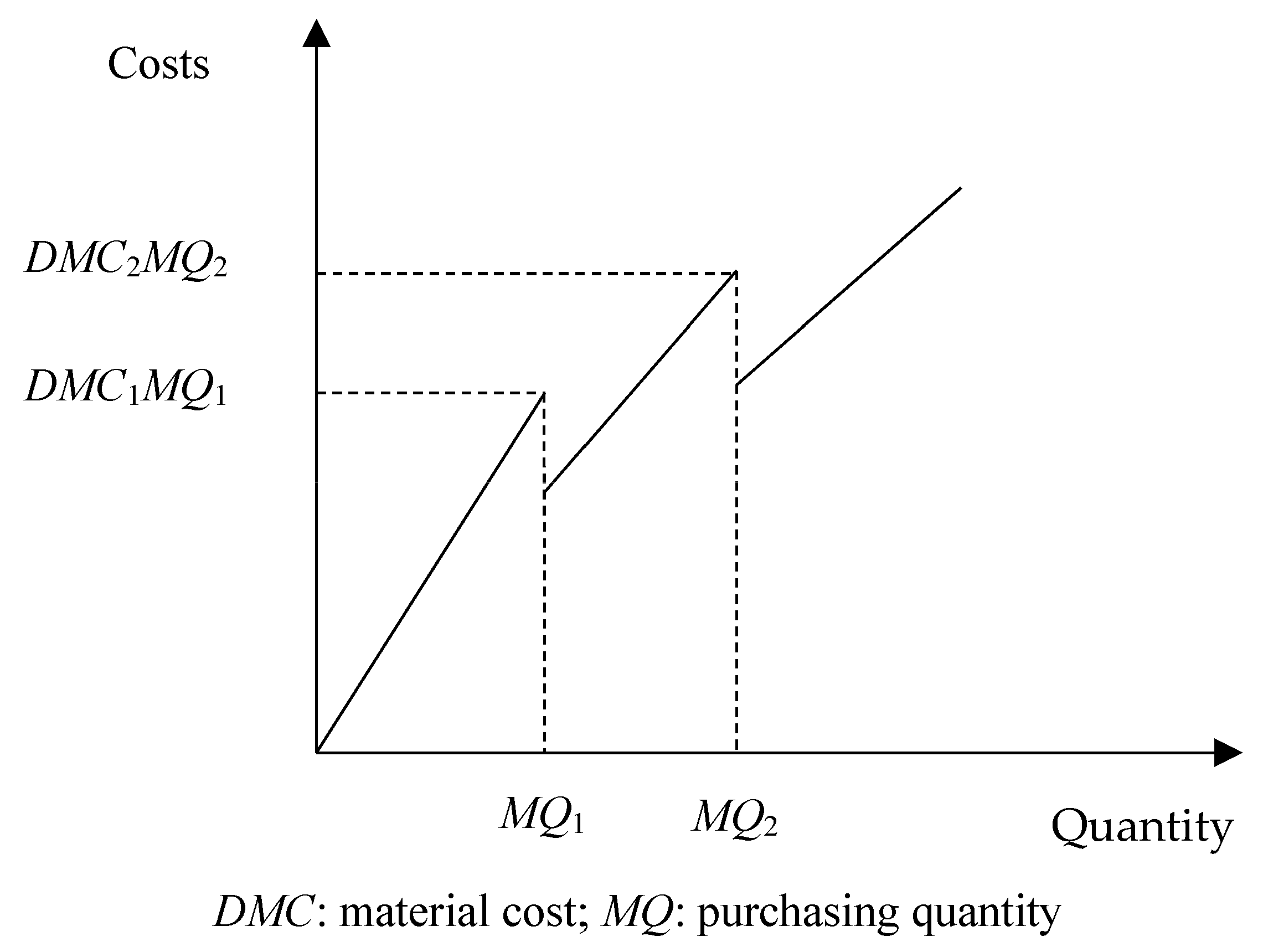
Direct material discounts are very common in the current commercial situation. Such discounts involve the buyer or customer having greater power to bargain with the seller or supplier, or the seller or supplier being willing to negotiate with the buyer as a long-term company partner or negotiate with the buyer. An contract has included the three purchase prices, namely the normal, the first discounted price, and the second discounted price. As shown in Figure 3, this section lists the multi-phase mode.
Constraints:
i = 1 n q i 1 P i t = D Q 1 t + D Q 2 t + D Q 3 t t = 1 , 2 T
0   D Q 1 t   α 0 t M Q 1 t = 1 , 2 T
α 1 t M Q 1 < D Q 2 t     α 1 t M Q 2 t = 1 , 2 T
α 2 t M Q 2 < D Q 3 t t = 1 , 2 T
α 0 t + α 1 t + α 2 t = 1 t = 1 , 2 T
In the case of multiple periods, the material requirement quantity specifies the upper limit quantity for the total period (UDQ):
t = 1 T D Q 1 t + D Q 2 t + D Q 3 t U D Q t = 1 , 2 T

3.1.3. Unit-Level Operations: Direct Labor Cost Function

Direct labor usually refers to the human resources used in the production line. The third group of formulas in Equation (1) H R 1 + ω 1 ( H R 2 H R 1 ) + ω 2 ( H R 3 H R 1 ) represents the direct labor cost function at the unit level. The correlation diagram and its restriction formulas are shown in Figure 4. This section lists the multi-phase mode.
Constraints:
i = 1 n o = 1 m u i o P i t C H 1 + ω 1 t ( C H 2 C H 1 ) + ω 2 t ( C H 3 C H 1 ) t = 1 , 2 T
ω 0 t β 1 t 0 t = 1 , 2 T
ω 1 t β 1 t β 2 t 0 t = 1 , 2 T
ω 2 t β 2 t 0 t = 1 , 2 T
ω 0 t + ω 1 t + ω 2 t = 1 t = 1 , 2 T
β 1 t + β 2 t = 1 t = 1 , 2 T

3.2. Multi-Phase Models without Allowance

3.2.1. Carbon Tax Function with Incremental Tax Rate without Allowance (Model A)

π = t = 1 T i = 1 n S i P i t t = 1 T ( D M C 1 D Q 1 t + D M C 2 D Q 2 t + D M C 3 D Q 3 t     i = 1 T j = 1 m M C j P i t q i j ) t = 1 T [ H R 1 + ω 1 t ( H R 2 H R 1 ) + ω 2 t ( H R 3 H R 1 ) ]     t = 1 T i = 1 n ( d o S i o B i o t + d o H o B o t ) t = 1 T ( φ 1 t T C C 1 + φ 2 t T C C 2 + φ 3 t T C C 3 ) i = 1 T F t
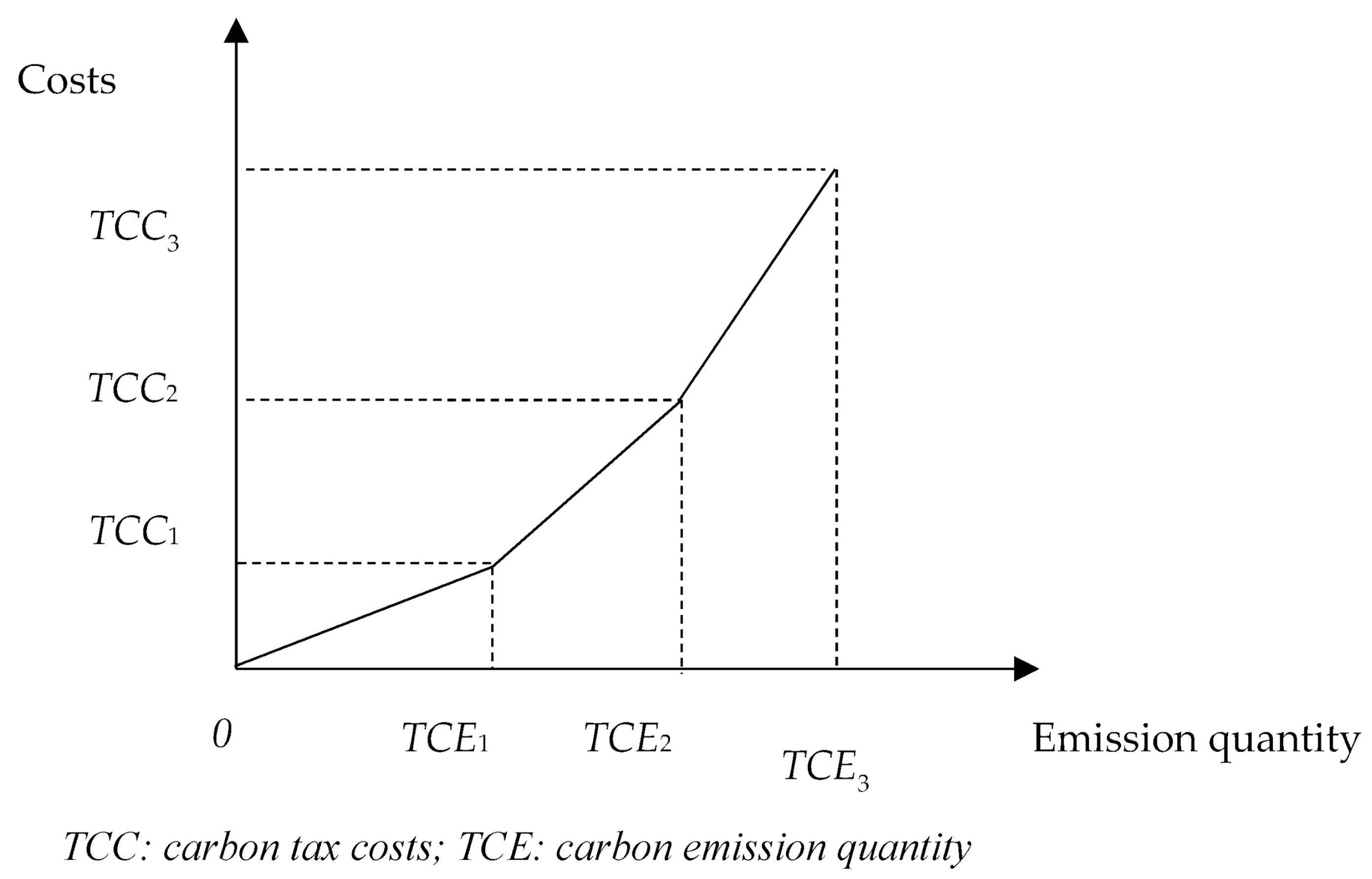
In this subsection, Model A1 takes into account a carbon tax, which is attached to each product, and it takes into account the carbon emissions cap set by the government, which is set in this model at 28,000 tons (CO2). The amount of product a company produces determines the amount of tax the company should pay. The correlation diagram and its restriction equations are shown in Figure 5. This section lists the multi-phase mode.
Constraints:
i = 1 n e i P i t = φ 1 t T C E 1 + φ 2 t T C E 2 + φ 3 t T C E 3 t = 1 , 2 T
φ 0 t γ 1 t 0 t = 1 , 2 T
φ 1 t γ 1 t γ 2 t 0 t = 1 , 2 T
φ 2 t γ 2 t γ 3 t   0 t = 1 , 2 T
φ 3 t γ 3 t 0 t = 1 , 2 T
φ 0 t + φ 1 t + φ 2 t + φ 3 t = 1 t = 1 , 2 T
γ 1 t + γ 2 t + γ 3 t = 1 t = 1 , 2 T
In the multi-period production decision mode, only the Model A1 needs to set this formula. Because there are no carbon rights trading, the total carbon emissions of multiple periods cannot exceed the upper limit of total carbon emissions of multiple periods stipulated by the government. Under the condition that carbon emission quotas or carbon rights can be stored or borrowed, the restriction formula of multi-phase enterprise carbon emission is less than or equal to the total carbon emission cap (GCE) stipulated by the government, which is as follows:
i = 1 n e i P i t i = 1 T G C E t t = 1 , 2 T
Functions:
f 1 ( C C E t ) = { c r 1 C C E t ,   0 C C E t T C E 1   T C C 1 + c r 2 ( C C E t T C E 1 ) ,   T C E 1 < C C E t T C E 2   T C C 2 + c r 3 ( C C E t T C E 2 ) ,   C C E t > T C E 2  

3.2.2. Carbon Tax Function with Incremental Tax Rate without Allowance (with Carbon Trading) (Model B)

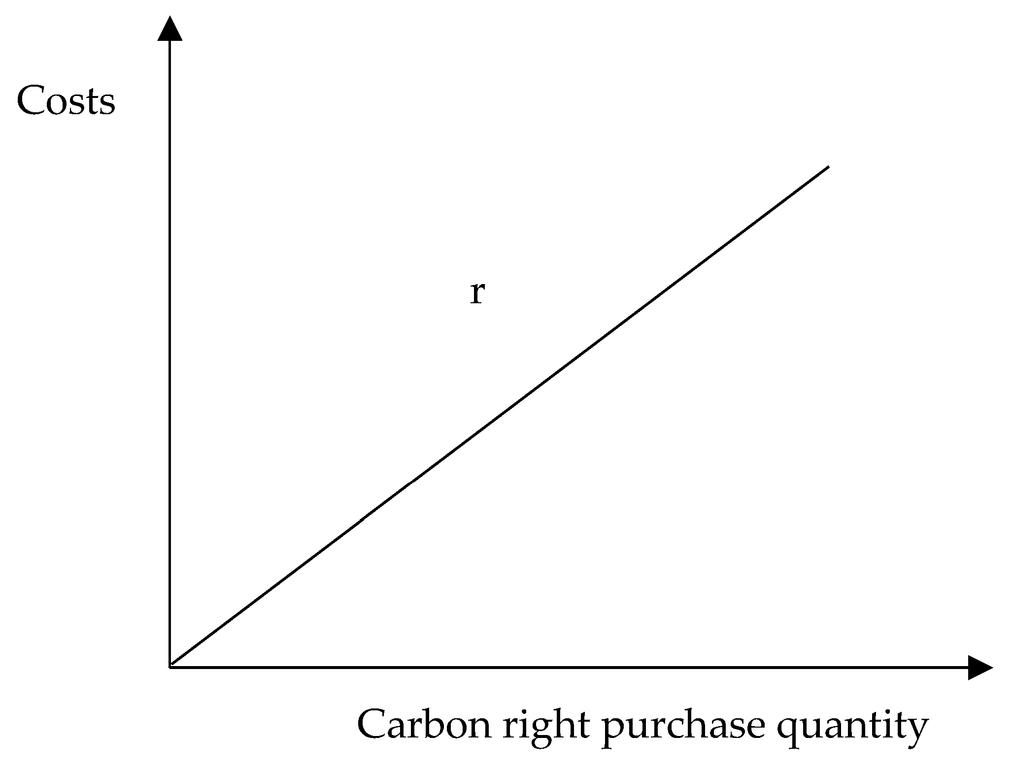
In the multi-period production decision-making model, the Model B adds a carbon right cost function. This must consider whether the total carbon emissions of the multi-period are less than or greater than the government regulations. In addition, the difference between GCEt and CCEt carbon emissions can still be compared in each period to indicate whether enterprises need to store or borrow carbon emissions in this period t. The correlation diagram and its restriction equations are shown in Figure 6.
π = t = 1 T i = 1 n S i P i t t = 1 T ( D M C 1 D Q 1 t + D M C 2 D Q 2 t + D M C 3 D Q 3 t     i = 1 T j = 1 m M C j P i t q i j ) t = 1 T [ H R 1 + ω 1 t ( H R 2 H R 1 ) + ω 2 t ( H R 3 H R 1 ) ] t = 1 T i = 1 n ( d o S i o B i o t + d o H o B o t ) { [ t = 1 T ( φ 1 t T C C 1 + φ 2 t T C C 2 + φ 3 t T C C 3 ) r ( i = 1 T G C E t t = 1 T C C E t ) ] λ 1 + [ t = 1 T ( φ 1 t T C C 1 + φ 2 t T C C 2 + φ 3 t T C C 3 ) + r ( t = 1 T C C E t i = 1 T G C E t ) ] λ 2   } i = 1 T F t
Constraints:
t = 1 T i = 1 n e i P i t = A C Q 1 + A C Q 2 = i = 1 T C C E t t = 1 , 2 T
0 A C Q 1 M Q λ 1 t = 1 , 2 T
M Q λ 2 < A C Q 2 ( M Q + T M B R ) λ 2 t = 1 , 2 T
λ 1 + λ 2 = 1 t = 1 , 2 T
Function:
f 2 ( C C E t G C E t ) = r ( C C E t G C E t )

3.3. Multi-Phase Modes with Allowance

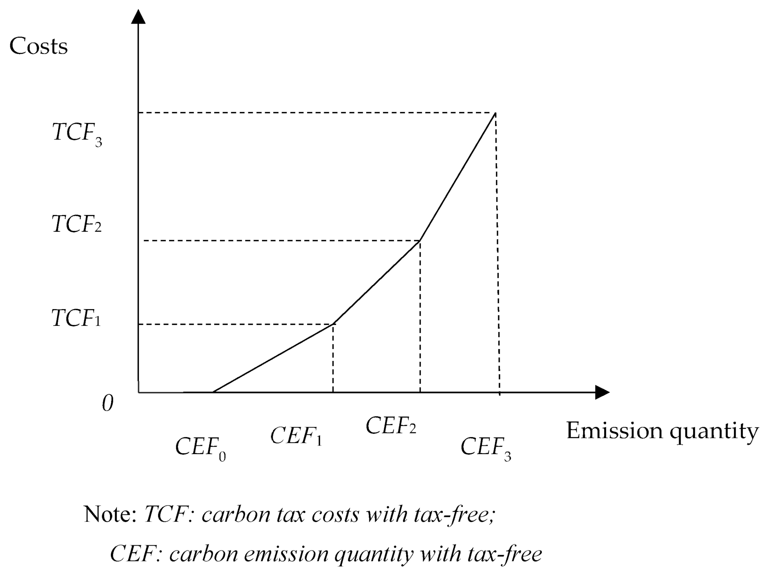
3.3.1. Carbon Tax Function with Incremental Incremental Tax Rate with Allowance (Model C)

In this subsection, Model C considers the carbon tax as a carbon tax function with an exemption amount and considers the carbon emission cap set by the government. This section lists the multi-phase mode.
π = t = 1 T i = 1 n S i P i t t = 1 T ( D M C 1 D Q 1 t + D M C 2 D Q 2 t + D M C 3 D Q 3 t     i = 1 T j = 1 m M C j P i t q i j ) t = 1 T [ H R 1 + ω 1 t ( H R 2 H R 1 ) + ω 2 t ( H R 3 H R 1 ) ] t = 1 T i = 1 n ( d o S i o B i o t + d o H o B o t ) t = 1 T ( σ 1 t T C F 1 + σ 2 t T C F 2 + σ 3 t T C F 3 ) i = 1 T F t
Constraints:
i = 1 n e i P i t C E F 0 + σ 1 t ( C E F 1 C E F 0 ) + σ 2 t ( C E F 2 C E F 0 ) + σ 3 t ( C E F 3 C E F 0 ) t = 1 , 2 T
σ 0 t μ 1 t 0 t = 1 , 2 T
σ 1 t μ 1 t μ 2 t 0 t = 1 , 2 T
σ 2 t μ 2 t μ 3 t   0 t = 1 , 2 T
σ 3 t μ 3 t 0 t = 1 , 2 T
σ 0 t + σ 1 t + σ 2 t + σ 3 t = 1 t = 1 , 2 T
μ 1 t + μ 2 t + μ 3 t = 1 t = 1 , 2 T
In the multi-period production decision mode, only the Model C needs to set this formula. Because there are no carbon rights trading, the total carbon emissions of multiple periods cannot exceed the upper limit of total carbon emissions of multiple periods stipulated by the government.

3.3.2. Carbon Tax Function with Incremental Incremental Tax Rate with Allowance (with Carbon Trading) (Model D)

In the multi-period production decision-making model, the Model D adds a carbon right cost function. This must consider whether the total carbon emissions of the multi-period are less than or greater than the government regulations. The correlation diagram and its restriction equations are shown in Figure 7.
π = t = 1 T i = 1 n S i P i t t = 1 T ( D M C 1 D Q 1 t + D M C 2 D Q 2 t + D M C 3 D Q 3 t     i = 1 T j = 1 m M C j P i t q i j ) t = 1 T [ H R 1 + ω 1 t ( H R 2 H R 1 ) + ω 2 t ( H R 3 H R 1 ) ] t = 1 T i = 1 n ( d o S i o B i o t + d o H o B o t ) { [ t = 1 T ( σ 1 t T C F 1 + σ 2 t T C F 2 + σ 3 t T C F 3 ) r ( i = 1 T G C E t t = 1 T C C E t ) ] λ 1 + [ t = 1 T ( σ 1 t T C F 1 + σ 2 t T C F 2 + σ 3 t T C F 3 ) + r ( t = 1 T C C E t i = 1 T G C E t ) ] λ 2   } i = 1 T F t
The multi-period total carbon emission cap is used as the basis for enterprises to purchase carbon rights. λ 1 and λ 2 are SOS1 variables; when one of these variables is set to 1, the other variables must be exactly zero. If λ 1 = 1, then λ 2 = 0, see Equation (40); ACQ1 ≥ 0 and ACQ1MQ, see Equation (38), which means that the total carbon emission is lower than the limit set by the government, so companies will not need buy additional carbon rights.
Constraints:
t = 1 T i = 1 n e i P i t = A C Q 1 + A C Q 2 = i = 1 T C C E t t = 1 , 2 T
0 A C Q 1 M Q λ 1 t = 1 , 2 T
M Q λ 2 < A C Q 2 ( M Q + T M B R ) λ 2 t = 1 , 2 T
λ 1 + λ 2 = 1 t = 1 , 2 T
Function:
f 5 ( C C E t G C E t ) = r ( C C E t G C E t )
TMBR Maximum number of carbon rights purchased in multi-period model

4. Research Analysis

In this section, according to the actual data, the best product combination in each model will be calculated. The chosen example company is an internationally renowned company with a strong focus on environmental sustainability. Recently, local governments announced carbon taxes and restrictions on carbon rights in future policies. This policy will have a huge impact on the company’s bottom line, even affecting the mix of original products. Therefore, this paper presents an example business to help businesses find possible product combinations under the new carbon tax and carbon entitlement policies. This paper also proposes different combinations of carbon taxes and carbon rights and compares each model, which will not only help companies better understand the differences, but also help governments choose which policies they should consider adopting. LINGO is the best software to solve this complex situation.

4.1. Sample Data

The company mainly produces three products: car rims (product 1, P = 1), truck rims (product 2, P = 2), and custom rims (product 3, P = 3). According to company policy, products 1 and 2 are make-to-stock (MTS) and product 3 is make-to-order (MTO), which means that products 1 and 2 require minimum production volume constraints, and usually car rims will be larger than truck wheels in use inventory. Since product 3 is a customized product, there is an upper limit on the production quantity. To ensure consistency, this study makes the following assumptions. All jobs in this ABC production process are divided into unit jobs and batch jobs. The selling price of the units remains unchanged. All machines and labor are 100% utilization: no breakdowns or other mishaps. All material costs remain the same, but the example company has control over the supplier, and the agreement discounts the material cost, which will directly affect the company’s final profit, and the agreement will not lapse during this period, as shown in the last column of Table 2.
Each operation has its capacity limit as shown in the last column of Table 3 and Table 4, while carbon emissions are calculated in tons.

4.2. Data Analysis

Model comparison and analysis are performed based on the sample data in Table 2, Table 3, Table 4 and Table 5, the best results of each model in Table 6, Table 7, Table 8 and Table 9, and the values used in the objective function and related constraints.

4.2.1. Carbon Tax Function with Incremental Incremental Tax Rate without Allowance (Model A)

The optimal solution, objective function, and related constraints of the basic production planning model under the ABC method of Model A are shown in Table 6.
Model B increases the carbon entitlement function. The optimal solution, objective function, and related constraints of Model B are shown in Table 7. The maximum profit is $28,886,270, an increase of $798,160 over model 1. The production volumes of the three products are 2000, 5058, and 5628, respectively. Truck rims (product 2) have significantly increased production due to the carbon rights trading mechanism. Through this model, it can be understood that if the government adopts the carbon rights trading mechanism, enterprises will have more profits and are more flexible than the general model.

4.2.2. Carbon Tax Function with Incremental Incremental Tax Rate with Allowance (Model C)

The optimal solution, objective function, and related constraints of the basic production planning model under the ABC method of Model C are shown in Table 8.
Model D increases the carbon entitlement function. The optimal solution, objective function, and related constraints of Model D are shown in Table 9. Through this model, it can be understood that if the government adopts the carbon rights trading mechanism, enterprises will have more profits and are more flexible than the general model, and because this model has a duty-free allowance, it is more attractive and an incentive for companies to produce more products.

4.2.3. Model Comparison

In terms of the quantity of goods, Model A and Model C produce the same quantity of goods, which may be due to setting the same upper limit of carbon emissions. Therefore, in order to achieve the same upper limit and product mix. In addition, the same is true for Model B, Model D.
In terms of carbon emissions, Model A and Model C will produce the carbon emissions stipulated by the government, and Model B and Model D will exceed the upper limit of emissions. By purchasing carbon rights to produce more products, the company will maximize profits. After comparing whether there is a carbon rights trading model, as explained in Section 4.2, we can understand the carbon rights trading mechanism, so that companies can flexibly adjust their output. The carbon trading tax rate in this study is set at $250. The result of running through the LINGO program is that more production is used to purchase carbon rights; if the carbon trading tax rate is increased, companies may obtain more profits by selling carbon rights instead of producing more products. In terms of carbon tax cost, for the comparison of models with carbon rights trading, the highest cost is Model C which is in line with the actual situation. This model is a continuous carbon tax function with no tax allowance and carbon rights trading. In terms of the cost of carbon rights, only Model C purchased 2000 carbon rights, while Model D was 4951. In the parts of material purchase quantity, labor cost, and labor hours, Model A and Model C will get the same results.

4.3. Multi-Period Sensitivity Analysis

Model A and Model C comparison of single-phase model as shown in Table 10. In the multi-period model, the parameter settings of the single-period model are extended, and the following two conditions are considered: (1) In the case of multiple periods, under the condition that carbon emission quotas or carbon rights can be stored or borrowed, they have an impact on the production decisions and total profits of each model. (2) In the case of multiple periods, the upper limit of the total period specified by the material demand quantity and the period consumption, the impact of the above two on the production decision and profit of each model, the relevant parameter settings are shown in Table 1 and Table 2. The research results of this paper take the Model D as an example and compare the carbon emissions cap with the original government’s carbon emissions cap under the condition that carbon emissions can be stored or borrowed to illustrate the impact of government policy formulation on corporate profits and carbon tax costs.
Taking Model D as an example, as shown in Table 11, the original data results set the carbon emission cap at 28,000 in the first phase, and the profit obtained is $28,923,600; in the second phase, the carbon emission cap is 25,200, and the profit is $28,557,480; in the third phase, the carbon emission cap was set at 22,400, and the profit obtained was $27,800,720. Overall, due to the fact that the carbon emission cap decreased gradually, the profit also decreased gradually.

4.4. Review

As shown in Table 10 these two elements are very sensitive and will experience some churn if any other resources change throughout the production environment. Even if a person leaves the job or a machine breaks down, it can lead to different outcomes. From the perspective of enterprises, they will prefer the model with higher profits, so Model D is the best model. This model has preferential tax exemptions and is more attractive to enterprises; from the government’s point of view, the goal is to allow enterprises to reduce carbon emissions, so Model A and Model C have the same effect. If the government pursues the largest carbon tax revenue, the Model A will have a greater impact on the government’s treasury. The carbon tax rate data assumed in this paper not only refer to the World Bank Group, but also refer to the pricing price in China. The implementation of the actual government is arranged and approved according to the fair price of each country. These regimes are very likely to happen in the real world in the future, and managers should pay more attention to the impact of carbon taxes and carbon rights. The results obtained show that for every 10% increase in the change in the unit cost of carbon rights, the profit decreases by 0.36%, and the impact of carbon rights on the profit is not much changed. When setting carbon rights, the government can consider the impact on corporate profits and set a reasonable price. In the multi-period sensitivity analysis, the original carbon emission cap and the storage and borrowing system are compared, and it is found that the profit and product production are similar, but the enterprise can make multi-phase deployment according to the carbon emission storage and borrowing system.
As mentioned above, carbon taxes and carbon rights affect not only a company’s profits but also its product mix. As pricing carbon emissions becomes the future trend in countries around the world, companies should start thinking about reducing their total carbon emissions across the production process, rather than doing nothing and just seeing taxes reduce overall profits. Governments must also carefully consider whether tax rates and carbon caps should vary by industry, and some industries may require more carbon emissions because of their size or other reasons. In addition, the government should think about whether to only impose a carbon tax or set up carbon trading, and which carbon tax or carbon right model should be selected. Once the policy is released, it will have a huge impact on businesses and even citizens. If the tax rate is too high, companies may move their production plants to other countries with no or less carbon tax, although the government will receive huge tax revenue to protect the environment. If the tax rate is too low, the benefits of environmental protection will not meet expectations. If the cost of taxation is reflected in future product prices, there may be derivative problems.

5. Conclusions and Suggestion

Environmental concerns continue to expand, and the United Nations Framework Convention on Climate Change (UNFCCC) announced the Paris Agreement in 2015 with a common goal: to confront the problem of global warming. Governments implementing relevant policies also face considerable work in dealing with environmental issues. However, countries implementing relevant policies generate less than 20% of global greenhouse gases. This article is based on an extended study of the green job costing system for the aluminum-alloy rim industry under Industry 4.0 released in 2019 [11]. This paper proposes four green ABC production planning models, which are the carbon tax model with an incremental tax rate without allowance, an incremental tax rate without allowance and the carbon trading model, the carbon tax model with an incremental tax rate with allowances, and an incremental tax rate with allowances and the carbon trading model. The results obtained show that for every 10% increase in the change in the unit cost of carbon rights, the profit decreases by 0.36%, and the impact of carbon rights on the profit is not much changed. When setting carbon rights, the government can consider the impact on corporate profits and set a reasonable price. In the multi-period sensitivity analysis, the original carbon emission cap and the storage and borrowing system are compared, and it is found that the profit and product production are similar, but the enterprise can make multi-phase deployments according to the carbon emission storage and borrowing system. The main research contributions of this study include the following aspects: First, this study introduces the concept of net-zero transformation into the production optimization decision-making model, which further promotes the green and sustainable development of the production process. Second, based on the characteristics of multi-period production, this research establishes a multi-period production optimization decision-making model, which can help enterprises formulate more scientific and effective production plans. Finally, this study applies the aluminum wheel frame industry case to prove the practicability and effect of the model, which can help enterprises improve production efficiency and cost control.
All models contain basic cost functions such as direct labor, direct material costs, and batch level operations: material handling and setup functions, and machine labor constraints. In Model B and Model D, the carbon rights trading function is considered, respectively. LINGO was chosen because it is the best program for solving such complex mathematical problems. Future research directions can be expanded from the following aspects: First, the current multi-period production optimization decision-making model under the net-zero transformation is mainly used in the manufacturing industry, and it can be applied to a wider range of industries in the future, such as the service industry and agriculture, to increase its practical value. Secondly, the existing research results mainly focus on the theoretical basis and algorithm design of the model. In the future, the uncertainty and variability in the actual production process can be further considered to improve the accuracy and applicability of the model. Third, in addition to production efficiency and resource utilization efficiency, the impact of decision-making models on environmental protection and social benefits can be explored in the future. Finally, in the future, artificial intelligence technology can be integrated into the decision-making model, such as machine learning and deep learning, which can improve the intelligence of the model.

Funding

The authors would like to thank the Ministry of Science and Technology of Taiwan for financial support of this research under Grant No. MOST109-2410-H-008-029-MY2.

Institutional Review Board Statement

This article does not contain any studies with human participants or animals performed by any of the authors.

Data Availability Statement

Data sharing not applicable.

Conflicts of Interest

The author declares that he has no conflicts of interest in this paper.

Nomenclature

SymbolDefinition
πCompany’s maximum profit
SiUnit sales price of the i-th product
PiThe output of the i-th product
DMC1,DMC2, DMC3Under normal circumstances, the unit cost of materials (DMC1), the first-stage discounted cost (DMC2)
DQ1, DQ2,
DQ3
The quantity consumed under normal conditions (DQ1), the quantity of the first segment of the discount section (DQ2)
MCjj material unit cost
qijWhen producing a unit of product i, the amount of material j consumed
HR1,HR2, HR3Direct labor costs under normal circumstances (HR1), the first period of overtime cost (HR2), the second period of overtime cost (HR3)
ω0, ω1, ω2SOS2 variable, must be a set of positive variables, at most two variables can be non-zero
doWhen performing a unit of operation o operation cost
BoNumber of batch operations under material handling operations (o ∈ B)
MQEquivalent to the sum of GCE1 + GCE2 +…GCEt
TMBRMaximum number of carbon rights purchased in multi-period model
λ1, λ2, SOS1 variables
ACQ1In the multi-period model, it is decided whether the company wants to purchase carbon rights
Sioi product demand under setting operation (o ∈ B)
BioThe batch quantity of the i product under the set operation (o ∈ B)
FOther fixed costs of example company

References

  1. Atwoli, L.; Erhabor, G.E.; Gbakima, A.A.; Haileamlak, A.; Kayembe Ntumba, J.-M.; Kigera, J.; Mulaudzi, F.M. COP27 Climate Change Conference: Urgent action needed for Africa and the worldWealthy nations must step up support for Africa and vulnerable countries in addressing past, present and future impacts of climate change. Nutr. Rev. 2022, 23, 19–21. [Google Scholar] [CrossRef]
  2. Nag, A.K.; Joshi, R. COP 26: Accelerating Efforts Towards Emission Reduction And Net Zero Pledge. Manag. Account. J. 2022, 57, 68–70. [Google Scholar] [CrossRef]
  3. O’riordan, T. COP 26 and Sustainability Science. Environ. Sci. Policy Sustain. Dev. 2022, 64, 2–3. [Google Scholar] [CrossRef]
  4. Ohlendorf, N.; Jakob, M.; Minx, J.C.; Schröder, C.; Steckel, J.C. Distributional Impacts of Carbon Pricing: A Meta-Analysis. Environ. Resour. Econ. 2021, 78, 1–42. [Google Scholar] [CrossRef]
  5. Stavins, R.N. The Relative Merits of Carbon Pricing Instruments: Taxes versus Trading. Rev. Environ. Econ. Policy 2022, 16, 62–82. [Google Scholar] [CrossRef]
  6. Folkens, L.; Schneider, P. Responsible Carbon Resource Management through Input-Oriented Cap and Trade (IOCT). Sustainability 2022, 14, 5503. [Google Scholar] [CrossRef]
  7. Carmona, R.; Fehr, M.; Hinz, J.; Porchet, A. Market Design for Emission Trading Schemes. SIAM Rev. 2010, 52, 403–452. [Google Scholar] [CrossRef]
  8. Kara, M.; Syri, S.; Lehtilä, A.; Helynen, S.; Kekkonen, V.; Ruska, M.; Forsström, J. The impacts of EU CO2 emissions trading on electricity markets and electricity consumers in Finland. Energy Econ. 2008, 30, 193–211. [Google Scholar] [CrossRef]
  9. Hervert-Escobar, L.; López-Pérez, J.F. Production planning and scheduling optimization model: A case of study for a glass container company. Ann. Oper. Res. 2020, 286, 529–543. [Google Scholar] [CrossRef]
  10. Lin, B.; Wu, W.; Song, M. Industry 4.0: Driving factors and impacts on firm’s performance: An empirical study on China’s manufacturing industry. Ann. Oper. Res. 2019. [Google Scholar] [CrossRef]
  11. Tsai, W.-H.; Chu, P.-Y.; Lee, H.-L. Green Activity-Based Costing Production Planning and Scenario Analysis for the Aluminum-Alloy Wheel Industry under Industry 4.0. Sustainability 2019, 11, 756. [Google Scholar] [CrossRef]
  12. Quesado, P.; Silva, R. Activity-Based Costing (ABC) and Its Implication for Open Innovation. J. Open Innov. Technol. Mark. Complex. 2021, 7, 41. [Google Scholar] [CrossRef]
  13. Al-Dhubaibi, A.A.S. Optimizing the value of activity based costing system: The role of successful implementation. Manag. Sci. Lett. 2021, 11, 179–186. [Google Scholar] [CrossRef]
  14. Ruidas, S.; Seikh, M.R.; Nayak, P.K. A Production Inventory Model for Green Products with Emission Reduction Technology Investment and Green Subsidy. Process. Integr. Optim. Sustain. 2022, 6, 863–882. [Google Scholar] [CrossRef]
  15. Chen, X.; Yang, H.; Wang, X.; Choi, T.-M. Optimal carbon tax design for achieving low carbon supply chains. Ann. Oper. Res. 2020. [Google Scholar] [CrossRef]
  16. Ruidas, S.; Seikh, M.R.; Nayak, P.K. A production inventory model with interval-valued carbon emission parameters under price-sensitive demand. Comput. Ind. Eng. 2021, 154, 107154. [Google Scholar] [CrossRef]
  17. Holmen, J.S. ABC vs. TOC: It’s a matter of time. Strateg. Financ. 1995, 76, 37. [Google Scholar]
  18. Shapiro, J.F. Modeling and IT Perspectives on Supply Chain Integration. Inf. Syst. Front. 2001, 3, 455–464. [Google Scholar] [CrossRef]
  19. Das, S.K.; Green, J.A.S.; Kaufman, J.G. The development of recycle-friendly automotive aluminum alloys. JOM 2007, 59, 47–51. [Google Scholar] [CrossRef]
  20. Association, A. Aluminum: The Element of Sustainability—A North American Aluminum Industry Sustainability Report; Retrieved 30 April 2013; The Aluminum Association: Arlington, VA, USA, 2011. [Google Scholar]
  21. Liu, G.; Bangs, C.E.; Müller, D.B. Unearthing Potentials for Decarbonizing the U.S. Aluminum Cycle. Environ. Sci. Technol. 2011, 45, 9515–9522. [Google Scholar] [CrossRef]
  22. Sarkar, B.; Kar, S.; Basu, K.; Guchhait, R. A sustainable managerial decision-making problem for a substitutable product in a dual-channel under carbon tax policy. Comput. Ind. Eng. 2022, 172, 108635. [Google Scholar] [CrossRef]
  23. Luo, R.; Zhou, L.; Song, Y.; Fan, T. Evaluating the impact of carbon tax policy on manufacturing and remanufacturing decisions in a closed-loop supply chain. Int. J. Prod. Econ. 2022, 245, 108408. [Google Scholar] [CrossRef]
  24. Cooper, R.; Kaplan, R.S. Profit priorities from activity-based costing. Harv. Bus. Rev. 1991, 69, 130–135. [Google Scholar]
  25. Malmi, T. Activity-based costing diffusion across organizations: An exploratory empirical analysis of Finnish firms. Account. Organ. Soc. 1999, 24, 649–672. [Google Scholar] [CrossRef]
  26. Toyabe, S.; Kurashima, S.; Okada, M.; Akazawa, K.; Cao, P. A Modified Method of Activity-based Costing for Objectively Reducing Cost Drivers in Hospitals. Methods Inf. Med. 2006, 45, 462–469. [Google Scholar] [CrossRef]
  27. Lin, B.Y.-J.; Chao, T.-H.; Yao, Y.; Tu, S.-M.; Wu, C.-C.; Chern, J.-Y.; Chao, S.-H.; Shaw, K.-Y. How can activity-based costing methodology be performed as a powerful tool to calculate costs and secure appropriate patient care? J. Med. Syst. 2007, 31, 85–90. [Google Scholar]
  28. Tsai, W.-H.; Lai, S.-Y.; Hsieh, C.-L. Exploring the impact of different carbon emission cost models on corporate profitability. Ann. Oper. Res. 2022, 322, 41–74. [Google Scholar] [CrossRef]
  29. Kee, R.; Schmidt, C. A comparative analysis of utilizing activity-based costing and the theory of constraints for making product-mix decisions. Int. J. Prod. Econ. 2000, 63, 1–17. [Google Scholar] [CrossRef]
  30. Rand, G.K. Critical chain: The theory of constraints applied to project management. Int. J. Proj. Manag. 2000, 18, 173–177. [Google Scholar] [CrossRef]
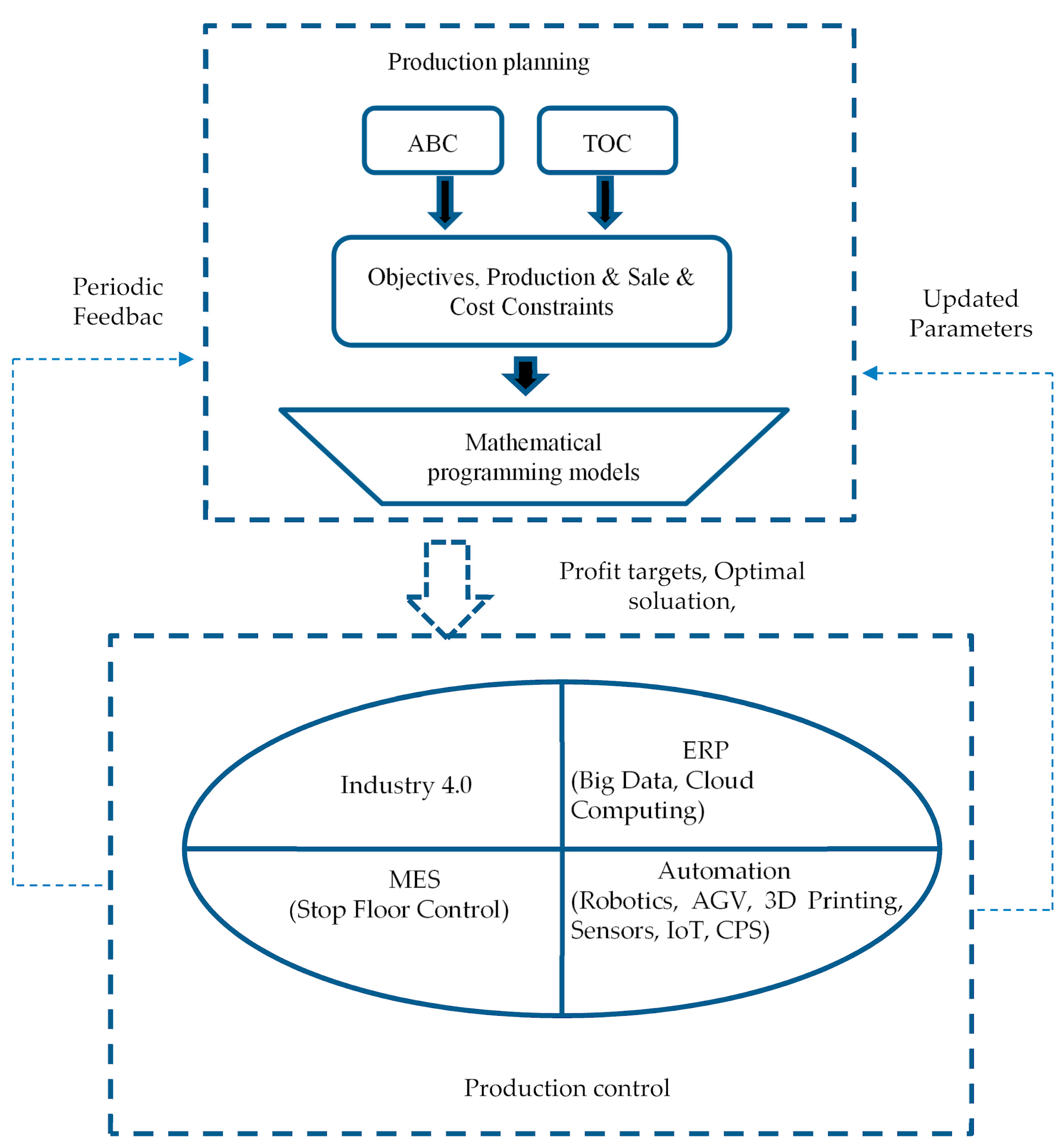
Figure 1. The relationship between mathematical modeling and Industry 4.0.
Processes 11 01439 g001
Figure 2. The common production process of aluminum rims.
Processes 11 01439 g002
Figure 3. Direct material discount function.
Processes 11 01439 g003
Figure 4. Direct labor cost function.
Processes 11 01439 g004
Figure 5. Carbon tax function with incremental tax rate without allowance.
Processes 11 01439 g005
Figure 6. Linear Carbon Entitlement Cost Function.
Processes 11 01439 g006
Figure 7. Carbon tax function with incremental tax rate with allowance.
Processes 11 01439 g007
Table 1. The features of the current research compared to other ones with a focus on solving production optimization decision.
ResearchersResearch Topic
Hervert-Escobar and López-Pérez, 2020 [9]Production planning and scheduling optimization model: a case of study for a glass container company.
Ruidas et al., 2021 [16]A production inventory model with interval-valued carbon emission parameters under price-sensitive demand.
Al-Dhubaibi, 2021 [13]Optimizing the value of activity-based costing system: The role of successful implementation.
Quesado and Silva, 2021 [12]Activity-based costing (ABC) and its implication for open innovation.
Ruidas et al., 2022 [14]A Production Inventory Model for Green Products with Emission Reduction Technology Investment and Green Subsidy.
Table 2. Example data.
Product ItemPiSiDirect Materials
at the Unit Level
Quantity
Cost
Maximum
/Minimum Production Volume
Selling Priceqi1
Aluminum Ingot (m = 1)
qi2
Coating (m = 2)
Car rim>20004000102MQ1 = 80,000D DMC1 = $70
Truck rim>10006000203MQ2 = 250,000 DMC2 = $69
Custom rims>2000,
<6000
8000104>250,000
DMC3 = $67
Table 3. Example data (operation capacity).
Product Itemc Material Handlingd SettingDirect Labor CostOther
Fixed
Costs
Decision-Making Mode of
Multi-Phase Production
H6ρ6Si7τi7CostLabor HoursSalary RateThe Upper Limit of Three-Phase Carbon EmissionThe Upper Limit of
Three-Phase
Material
Car rim17012HR1 = $7,022,400
HR2 = $14,018,400
HR3 = $23,337,600
CH1 = 52,800
CH2 = 79,200
CH3 = 105,600
$133/h
$177/h
$221 /h
F = 10,000,000GCE1 = 28,000
GCE2 = 25,200
GCE3 = 22,400
UDQ=39,000
Truck rim12
Custom rims2.51
Available capacityA6 = 8800A7 = 17,600
Note: c d6 = $2500/batch; d d7 = $200/batch.
Table 4. Example data (batch level operation).
Product ItemMachine HoursLabor Hours
rhi1
Casting
rhi2e
Heat treatment
rhi3
a CNC
rhi4
b CNC 2nd
Paintingui1
Casting
ui2
Heat treatment
ui3
a CNC
ui4
b CNC 2nd
ui5
Painting
Car rim23200.11.21.5100.3
Truck rim34300.11.72100.3
Custom rims2410.90.21.21.51.610.7
Available capacityCP1 = 46,200CP2 = 50,400CPCNC =18,900CP5 = 2070
Note: a The computer numerical control; b The second computer numerical control.
Table 5. Example data (carbon tax and right cost).
Product ItemAvailable
o Car RimTruck RimCustom RimsCapacity
Carbon tax with incremental tax rate without allowance (Model 1) ei1.523
CostTCC1 = $2,500,000TCC2 = $5,500,000TCC3 = $9,000,000
QuantityTCE1 = 10,000TCE2 = 20,000TCE3 = 30,000
Tax ratecr1 = $250/unitcr2 = $300/unitcr3 = $350/unit
Carbon tax with incremental incremental tax rate with allowance (Model 2) ei1.523
CostTCF1 = $2,500,000TCF2 = $5,500,000TCF3 = $9,000,000
QuantityCEF0 = 5000CEF1 = 15,000CEF2 = 25,000CEF3 = 35,000
Tax ratecrf1 = $250/unitcrf2 = $300/unitcrf3 = $350/unit
Linear carbon right cost
Carbon right costr = $250/unit Maximum carbon emissions cap set by the governmentGCE = 28,000
QuantityMBR = 100,000
Table 6. The optimal solution, objective function, and related constraints of Model A.
[Optimal solution]
π = 28,088,110; P1 = 2006; P2 = 3624; P3 = 5914; DQ1 = 0; DQ2 = 151,680; DQ3 = 0; ω0 = 0.6656061; ω1 = 0.3343939; ω2 = 0; B6 = 2167; B17 = 1003; B27 = 1812; B37 = 5914; φ0 = 0; φ1 = 0; φ2 = 0.2001; φ3 = 0.7999; α1 = 0; α2 = 1; α3 = 0; β1 = 1; β2 = 0; γ1 = 0; γ2 = 0; γ3 = 1; CCE = 27,999
[Objective function]
Maximum π = 4000*P1 + 6000*P2 + 8000*P3 − (70*DQ1 + 69*DQ2 + 67*DQ3 − 100*P1 + 150*P2 + 200*P3) − [7,022,400 + ω1*6,996,000 + ω2*16,315,200] − 2500*B6 − 200*B17 − 200*B27 − 500*B37 −(2,500,000*φ1 + 5,500,000*φ1 + 9,000,000*φ2) – 10,000,000
[Constraints]
Direct material discount:Direct labor:
10*P1 + 20*P2 + 10*P3 = DQ1 + DQ2 + DQ34*P1 + 5*P2 + 6*P3 = 52,800 − ω1*26,400 − ω2*52,800
0 ≤ DQ1α0*200,000ω0β1 ≤ 0
α1*200,000 < DQ2α1*500,000ω1β1β2 ≤ 0
α2*500,000 < DQ3 ω2β2 ≤ 0
α0 + α1 + α2 = 1ω0 + ω1 + ω2 = 1
β1 + β2 = 1
Batch Level: Material Handling
10*P1 + 20*P2 + 10*P3 ≤ 70*B6Batch Level: Settings
1*B6 ≤ 8800P1 ≤ 2*B17
P2 ≤ 2*B27
Machine hours:P3 ≤ 1*B37
o = 1 : 2*P1 + 3*P2 + 2*P3 ≤ 46,2001*B17 + 1*B27 + 2.5*B37 ≤ 17,600
o = 2 : 3*P1 + 4*P2 + 3*P3 ≤ 50,400
o = 3, 4 : 1*P1 + 1*P2 + 1.9*P3 ≤ 18,900Min/Max demand:
o = 5 : 0.1*P1 + 0.1*P2 + 0.2*P3 ≤ 2070P1 > 2000; P2 > 1000; 6000 > P3 > 2000
Carbon tax with incremental incremental tax rate without allowance:
1.5*P1 + 2*P2 + 3*P3 = φ1*10,000 + φ2*20,000 + φ3*30,000
1.5*P1 + 2*P2 + 3*P3 ≤ 28,000
φ0γ1 ≤ 0
φ1γ1γ2 ≤ 0
φ2γ2γ3 ≤ 0
φ3γ3 ≤ 0
φ0 + φ1 + φ2 + φ3 = 1
γ1 + γ2 + γ3 = 1
Table 7. The optimal solution, objective function, and related constraints of Model B.
[Optimal solution]
π = 28,886,270; P1 = 2000; P2 = 5058; P3 = 5628; DQ1 = 0; DQ2 = 177,440; DQ3 = 0; ω0 = 0.4599242; ω1 = 0.5400758; ω2 = 0; B6 = 2535; B17 = 1000; B27 = 2529; B37 = 5628; φ0 = 0; φ1 = 0; φ2 = 0; φ3 =1; α1 = 0;α2 = 1; α3 = 0; β1 = 1; β2 = 0;γ1 = 0;γ2 = 0; γ3 = 1; GCE = 28,000; Ø1 = 0; Ø2 = 1; CQ1 = 0; CQ2 = 30,000
[Objective function]
Maximum π = 4000*P1 + 6000*P2 + 8000*P3 – (70*DQ1 + 69*DQ2 + 67*DQ3 – 100*P1 + 150*P2 + 200*P3) – [7,022,400 + ω1*6,996,000 + ω2*16,315,200] – 2500*B6 – 200*B17 – 200*B27 – 500*B37 – (2,500,000*φ1 + 5,500,000*φ1 +9,000,000*φ2 – 250*(GCECCE))* Ø1 – (2,500,000*φ1 + 5,500,000*φ1 + 9,000,000*φ2 + 250*(CCEGCE))* Ø2 – 10,000,000
[Constraints]
Direct material discount:Direct labor:
10*P1 + 20*P2 + 10*P3 = DQ1 + DQ2 + DQ34*P1 + 5*P2 + 6*P3 = 52,800 – ω1*26,400 – ω2*52,800
0 ≤ DQ1α0*200,000ω0β1 ≤ 0
α1*200,000 < DQ2α1*500,000ω1β1β2 ≤ 0
α2*500,000 < DQ3 ω2β2 ≤ 0
α0 + α1 + α2 = 1ω0 + ω1 + ω2 = 1
β1 + β2 = 1
Batch Level: Material Handling
10*P1 + 20*P2 + 10*P3 ≤ 70*B6Batch Level: Settings
1*B6 ≤ 8800P1 ≤ 2*B17
P2 ≤ 2*B27
Machine hours:P3 ≤ 1*B37
o = 1 : 2*P1 + 3*P2 + 2*P3≤ 46,2001*B17 + 1*B27 + 2.5*B37 ≤ 17,600
o = 2 : 3*P1 + 4*P2 + 3*P3 ≤ 50,400
o = 3, 4 : 1*P1 + 1*P2 + 1.9*P3 ≤ 18,900Min/Max demand:
o = 5 : 0.1*P1 + 0.1*P2 + 0.2*P3 ≤ 2070P1 > 2000; P2 > 1000; 6000 > P3 > 2000
Linear carbon rights:Carbon tax with incremental incremental tax rate without allowance:
1.5*P1 + 2*P2 + 3*P3 = CQ1 + CQ2 = CCE1.5*P1 + 2*P2 + 3*P3 = φ1*10,000 + φ2*20,000 + φ3*30,000
0 ≤ CQ1 ≤ 28,000*Ø11.5*P1 + 2*P2 + 3*P3 ≤ 28,000
28,000*Ø1 < CQ2 ≤ 128,000*Ø2φ0γ1 ≤ 0
Ø1 + Ø2 = 1φ1γ1γ2 ≤ 0
φ2γ2γ3 ≤ 0
φ3γ3 ≤ 0
φ0 + φ1 + φ2 + φ3 = 1
γ1 + γ2 + γ3 = 1
Table 8. The optimal solution, objective function, and related constraints of Model C.
[Optimal solution]
π = 29,838,110; P1 = 2006; P2 = 3624; P3 = 5914; DQ1 = 0; DQ2 = 151,680; DQ3 = 0;ω0 = 0.6656061; ω1 = 0.3343939; ω2 = 0; B6 = 2167; B17 = 1003; B27 = 1812; B37 = 5914; σ0 = 0; σ1 = 0; σ2 = 0.7001; σ3 = 0.2999; α1 = 0; α2 = 1; α3 = 0; β1 = 1; β2 = 0; μ1 = 0; μ2 = 0; μ3 = 1; CCE = 27,999
[Objective function]
Maximum π = 4000*P1 + 6000*P2 + 8000*P3 − (70*DQ1 + 69*DQ2 + 67*DQ3 − 100*P1 + 150*P2 + 200*P3) − [7,022,400 + ω1*6,996,000 + ω2*16,315,200] − 2500*B6 − 200*B17 − 200*B27 − 500*B37 − (2,500,000*σ1 + 5,500,000*σ1 + 9,000,000*σ2) − 10,000,000
[Constraints]
Direct material discount:Direct labor:
10*P1 + 20*P2 + 10*P3 = DQ1 + DQ2 + DQ34*P1 + 5*P2 + 6*P3 = 52,800 − ω1*26,400 − ω2*52,800
0 ≤ DQ1α0*200,000ω0β1 ≤ 0
α1*200,000 < DQ2α1*500,000ω1β1β2 ≤ 0
α2*500,000 < DQ3 ω2β2 ≤ 0
α0 + α1 + α2 = 1ω0 + ω1 + ω2 = 1
β1 + β2 = 1
Batch Level: Material Handling
10*P1 + 20*P2 + 10*P3 ≤ 70*B6Batch Level: Settings
1*B6 ≤ 8800P1 ≤ 2*B17
P2 ≤ 2*B27
Machine hours:P3 ≤ 1*B37
o = 1: 2*P1 + 3*P2 + 2*P3 ≤ 46,2001*B17 + 1*B27 + 2.5*B37 ≤ 17,600
o = 2: 3*P1 + 4*P2 + 3*P3 ≤ 50,400
o = 3, 4: 1*P1 + 1*P2 + 1.9*P3 ≤ 18,900Min/Max demand:
o = 5: 0.1*P1 + 0.1*P2 + 0.2*P3 ≤ 2070P1 > 2000; P2 > 1000; 6000 > P3 > 2000
Carbon tax with incremental incremental tax rate with allowance:
1.5*P1 + 2*P2 + 3*P3 ≤ 5000 + σ1*10,000 + σ2*20,000 + σ3*30,000
1.5*P1 + 2*P2 + 3*P3 ≤ 28,000
σ0μ1 ≤ 0
σ1μ1μ2 ≤ 0
σ2μ2μ3 ≤ 0
σ3μ3 ≤ 0
σ0 + σ1 + σ2 + σ3 = 1
μ1 + μ2 + μ3 = 1
Table 9. The optimal solution, objective function, and related constraints of Model D.
[Optimal solution]
π = 31,668,590; P1 = 2000; P2 = 6910; P3 = 5257; DQ1 = 0; DQ2 = 210,770; DQ3 = 0;ω0 = 0.1934848; ω1= 0.8065152; ω2 = 0; B6 = 3011; B17 = 1000; B27 = 3455; B37 = 5257; σ0 = 0; σ1 =0; σ2 = 0.2409; σ3 = 0.7591; α1 = 0;α2 = 1; α3 = 0; β1 = 1; β2 = 0; μ1 = 0; μ2 = 0; μ3 = 1; GCE = 28,000 ;Ø1 = 0; Ø2 = 1;CQ1 = 0;CQ2 = 32,591
[Objective function]
Maximum π = 4000*P1 + 6000*P2 + 8000*P3 − (70*DQ1 + 69*DQ2 + 67*DQ3 − 100*P1 + 150*P2 + 200*P3) − [7,022,400 + ω1*6,996,000 + ω2*16,315,200] − 2500*B6 − 200*B17 − 200*B27 − 500*B37 − (2,500,000*σ1 + 5,500,000*σ1 +9,000,000*σ2 − 250*(GCECCE))*Ø1 − (2,500,000*σ1 + 5,500,000*σ1 +9,000,000*σ2 +250*(CCE-GCE))*Ø2 −10,000,000
[Constraints]
Direct material discount:Direct labor:
10*P1 + 20*P2 + 10*P3 = DQ1 + DQ2 + DQ34*P1 + 5*P2 + 6*P3 = 52,800 − ω1*26,400 − ω2*52,800
0 ≤ DQ1α0*200,000ω0β1 ≤ 0
α1*200,000 < DQ2α1*500,000ω1β1β2 ≤ 0
α2*500,000 < DQ3 ω2β2 ≤ 0
α0 + α1 + α2 = 1ω0 + ω1 + ω2 = 1
β1 + β2 = 1
Batch Level: Material Handling
10*P1 + 20*P2 + 10*P3 ≤ 70*B6Batch Level: Settings
1*B6 ≤ 8800P1 ≤ 2*B17
P2 ≤ 2*B27
Machine hours:P3 ≤ 1*B37
o = 1: 2*P1 + 3*P2 + 2*P3 ≤ 46,2001*B17 + 1*B27 + 2.5*B37 ≤ 17,600
o = 2: 3*P1 + 4*P2 + 3*P3 ≤ 50,400
o = 3, 4: 1*P1 + 1*P2 + 1.9*P3 ≤ 18,900Min/Max demand:
o = 5: 0.1*P1 + 0.1*P2 + 0.2*P3 ≤ 2070P1 > 2000; P2 > 1000; 6000 > P3 > 2000
Linear carbon rights:Carbon tax with incremental incremental tax rate with allowance:
1.5*P1 + 2*P2 + 3*P3 = CQ1 + CQ2 = CCE1.5*P1 + 2*P2 + 3*P3 ≤ 5000 + σ1*10,000 + σ2*20,000 + σ3*30,000
0 ≤ CQ1 ≤ 28,000*Ø11.5*P1 + 2*P2 + 3*P3 ≤ 28,000
28,000*Ø1 < CQ2 ≤ 128,000*Ø2σ0μ1 ≤ 0
Ø1 + Ø2 = 1σ1μ1μ2 ≤ 0
σ2μ2μ3 ≤ 0
σ3μ3 ≤ 0
σ0 + σ1 + σ2 + σ3 = 1
μ1 + μ2 + μ3 = 1
Table 10. Model A and Model C comparison of single-phase model.
ModelProfitQuantity of GoodsCarbon EmissionCarbon TaxCarbon RightsThe Cost
of Carbon Rights
Quantity of Material
Purchased
Labor
Cost
Labor Hours
A128,088,110P1 = 2006;
P2 = 3624;
P3 = 5914
27,9998,299,65000151,6809,361,82061,628
A228,886,270P1 = 2000;
P2 = 5058;
P3 = 5628
30,0009,000,000200050,000177,44010,800,77067,058
B129,838,110P1 = 2006;
P2 = 3624;
P3 = 5914
27,9996,549,65000151,6809,361,82061,628
B231,668,590P1 = 2000;
P2 = 6910;
P3 = 5257
32,5918,156,85045911,147,750210,77012,664,78074,092
Table 11. Carbon emissions from Model D compared to original carbon cap costs under storable or borrowed conditions.
PeriodProfitQuantity of GoodsCarbon EmissionCarbon
Tax
Carbon RightsThe Cost
of Carbon Rights
Quantity of MATERIALCost of MaterialLabor HoursLabor CostBatch Cost
Carbon emission caps set for each period
128,923,600P1 = 4000
P2 = 1200
P3 = 6000
26,4005,990,000(1600)(400,000)124,00010,336,00058,0008,400,4007,950,000
228,557,480P1 = 3016
P2 = 2184
P3 = 6000
26,8926,162,2001692423,000133,84011,064,16058,9848,661,1608,300,000
327,800,720P1 = 3184
P2 = 2016
P3 = 6000
26,8086,132,80044081,102,000132,16010,939,84058,8168,616,6408,240,000
Lump sum85,281,800 80,10018,285,00045001,125,000390,00032,340,000175,80025,678,20024,490,000
Carbon emissions that can be stored or borrowed per period
129,091,930P1 = 3506
P2 = 1694
P3 = 6000
26,6476,076,450(1353)(338,250)128,94010,701,56058,4948,531,3108,125,000
228,492,930P1 = 3206
P2 = 1994
P3 = 6000
26,7976,128,9501597399,250131,94010,923,56058,7948,610,8108,232,500
327,696,940P1 = 3488
P2 = 1694
P3 = 6000
26,6566,079,60042561,064,000129,12010,714,88058,4228,536,0808,132,500
Lump sum85,281,800 80,10018,285,00045001,125,000390,00032,340,000175,71025,678,20024,490,000
Disclaimer/Publisher’s Note: The statements, opinions and data contained in all publications are solely those of the individual author(s) and contributor(s) and not of MDPI and/or the editor(s). MDPI and/or the editor(s) disclaim responsibility for any injury to people or property resulting from any ideas, methods, instructions or products referred to in the content.