Abstract
In the present paper, a mathematical model is built and implemented to describe the trajectories of mass inventories, pressures and polymer properties with emphasis on final particle size distributions of industrial scale poly(vinyl chloride) suspension polymerization reactors. The model comprises the mass balances, statistical moment balances, equilibrium relationships and population balance equations. A discretization scheme is employed to transform the integro-differential equations resulting from the population balance model into a system of differential equations. The obtained results show, for the first time, that classical breakage and coalescence kernels described in the literature can provide very good fittings of actual industrial scale data when coupled with proper parameter estimation procedures, so that the proposed model is able to represent the available operation data with good accuracy at distinct conditions. Particularly, it is also shown that the use of a top condenser for control of the reactor temperature can lead to changes of parameters that control the particle size distributions.
1. Introduction
Poly(vinyl chloride) (PVC) belongs to the group of the most important commercial plastic materials. It is surpassed only by poly(ethylene) (PE) and poly(propylene) (PP) in terms of worldwide production [1]. From an economic standpoint, the global PVC market is expected to grow at a compounded annual growth rate (CAGR) of 4.4% from 2022 to 2030 reaching 9.95 billion dollars [2]. Furthermore, the economic importance of PVC is linked to its numerous areas of application [3,4,5,6,7,8]. Mijangos et al. [9] and Abreu et al. [10] performed reviews on the current status of PVC production emphasizing the problems that still exist and the perspectives for the future.
Nearly 80% of the worldwide PVC production is achieved through suspension polymerization [11]. According to this polymerization technique, the monomer and oil soluble initiators are dispersed in water (continuous phase) by proper agitation and suspending agents [12,13,14]. Afterwards, the reaction starts when the temperature is increased until the desired value and the polymer chains are formed inside the dispersed monomer droplets [12,13]. Consequently, at the microscopic level, each monomer droplet behaves as a small bulk reactor [13]. Therefore, bulk and suspension polymerizations share closely akin kinetic features [15].
The continuous aqueous phase has the task of improving heat transfer and reducing the viscosity of the suspension [13]. The level of agitation [16,17] and surfactant type and concentration [18,19] make the control of particle morphology possible and it is one of the reasons by which this technology is succesfully widespread. Commercially, spherical polymer particles with characteristic diameters ranging from 50 to 500 m are produced [20]. Furthermore, the particle porosity plays an important role in the final application of the resin, since it controls the rates of plasticizer adsorption and the interaction of the resin with the plasticizers, affecting the performances of processing stages and the final properties of PVC pieces [21]. This explains the interest in the development of techniques to monitor the properties of the particles inside the reactor [22,23,24,25,26].
Given the importance of PVC particle morphology, the present work builds and implements a model to describe the trajectories of mass inventories, pressures and polymer properties with emphasis on particle size distributions, of industrial scale batch suspension polymerization reactors for the production of poly(vinyl chloride). In order to achieve this, firstly, a kinetic model is developed and validated with actual industrial data. Subsequently, a population balance model is combined with the latter to describe the particle size distributions in terms of the operational conditions and suspension properties. It is important to emphasize, as shown in the following section, that this is the first time that a population balance is validated with actual industrial data to represent product size distributions in large-scale PVC rectors.
2. Literature Review
Before addressing the proposed mathematical model development, a comprehensive literature review that covers the area of PVC polymerization modeling and population balances is provided. Regarding the population balances, the review focuses initially on some of the basic concepts, while afterwards the subject is narrowed down to applications on suspension polymerizations.
2.1. PVC Polymerization Modeling
The literature related to modeling of PVC polymerization dates back to the 1960’s. Firstly, Talamini [27] investigated the bulk polymerization of vinyl chloride monomer (VCM) and proposed a currently classical two-phase model to describe the conversion of monomer. According to this two-phase model, the polymerization takes place in the concentrated phase (polymer-rich) and in the diluted phase (monomer-rich) at different rates. The reaction rate in the concentrated phase is higher due to the well-know gel effect that reduces the rates of termination of polymer radicals in the polymer particles. This model was able to predict experimental data accurately up to conversions of 30%.
Crosato-Arnaldi et al. [15], following the work by Talamini [27], studied bulk and suspension polymerizations of VCM using different initiators. These authors concluded that the autocatalytic behavior observed in VCM polymerization is due only to phase separation and does not depend on the type of initiator. It was observed that the equation employed to describe the overall conversion agreed accurately with available data up to conversions of 50-60%; however, beyond this value, the fit was not satisfactory. In spite of that, the authors did not provide a clear explanation to this fact. Additionally, it was shown that the kinetics of bulk and suspension polymerizations are equivalent. This was concluded based on the observation that the conversion curves of bulk and suspension polymerizations overlap when plotted against time multiplied by the square root of the initiator concentration. Data related to VCM polymerizations and reported in prior literature were fitted with fair accuracy by the developed model.
Abdel-Alim and Hamielec [28] investigated the bulk polymerization of VCM with emphasis on molar mass and molar mass distributions (MMD). These authors developed a model to predict conversion based on the model presented originally by Talamini [27]. In their model, the effects of volume change and of molecular diffusion on the kinetic constants were also considered. By doing so, the rate of propagation was assumed to be null near the glass transition point. Consequently, their model was able to accurately predict conversions in the range where the model proposed by Crosato-Arnaldi et al. [15] was not able to.
Ugelstad et al. [29] studied the bulk polymerizations of VCM. These investigators considered the possible effects of adsorption and desorption of radicals from the polymer-rich phase. Furthermore, based on experimental data, it was concluded that the model used to predict the conversion was more accurate than the one proposed by Crosato-Arnaldi et al. [15]. In fact, the new model was equivalent to the one proposed by Crosato-Arnaldi et al. [15] only if two assumptions were made. Firstly, if the rate of termination in the polymer-rich phase was lower than its counterpart in the monomer-rich phase, which was true according to available experimental data. Secondly, if the volume change during polymerization was neglected. In fact, during the development of the model equations used to predict the conversion, it was assumed that the volumes of the phases could vary with conversion, which is an aspect that can not be disregarded in bulk and, consequently, suspension VCM polymerizations.
Kuchanov and Bort [30] performed a critical analysis of the previously published manuscripts and kinetic data regarding bulk and suspension VCM polymerizations. These authors emphasized that several authors made fundamental mistakes related to some of the assumptions used to derive the kinetic equation to explain the bulk and suspension polymerizations of VCM. One of the errors, according to these authors, was the use of homogeneous kinetic theory in an inherently heterogeneous reaction system. Additionally, these authors argued that Talamini’s assumption [15,27] that the radical concentration in both phases present was independent of conversion could not be supported by available experimental data. Furthermore, the assumption that the radicals were not initiated inside the polymer particles was also criticized, as this assumption was inadmissible out the low conversion range.
Hamielec et al. [31] focused on the effects of diffusion limitations on the kinetic constants of the reaction. These authors proposed a detailed kinetic mechanism to explain VCM polymerization, and included parameters in the rate constants to account for the effects of diffusion limitations. According to these authors, it was well established that the rate of termination decreased with conversion, resulting in increasing number of radicals, which explained the autocatalytic behavior noted by previous investigators. Additionally, as the glass transition point of the polymer is approached, the rate of propagation falls due to the effect of decreased free volume, which impairs the mobility of the monomer molecules to the active centers. In fact, these observations are very important for the operation of batch reactors because, as the conversion approaches higher values, the molecular properties (molar mass and branching distributions, for instance) of PVC, which relate to thermal stability, are deteriorated due to the mentioned diffusion effects. Based on these observations, the authors proposed operation policies to operate a batch reactor in a fashion designed to ensure the improvement of the final molecular properties.
Sidiropoulou and Kiparissides [32] developed a general model for the suspension VCM polymerization to predict the main molecular properties of PVC. The employed kinetic mechanism was identical to the one used by Hamielec et al. [31]. More specifically, the proposed model comprised the mass balances of growing and terminated radicals, initiator and monomer. To overcome the problem of solving a large number of equations, the authors employed the method of moments to obtain a smaller number of ordinary differential equations. The authors emphasized that their model was a generalization of previous models. In order to validate their work, simulations were performed and the results were compared to results provided by previous models found in the literature. Lastly, these investigators also considered the effects of diffusion control at higher conversions. For comparative purposes, the authors quantified the deviations caused by disregarding diffusion effects on kinetic rates.
Pinto [33] developed a simplified model based on the work of Abdel-Alim and Hamielec [28] and investigated strategies to carry out polymerization at constant rate in a batch reactor. The author investigated several strategies and concluded that it was almost impossible to keep the polymerization rate constant in an industrial batch reactor due to heat transfer limitations. The author also pointed out that a proper initiator choice and feed strategy would help in this undertaking. In posterior works, Pinto [34,35] performed a dynamic analysis in continuous VCM polymerizations in a stirred vessel. The author was able to identify the ranges in the parameter space where complex phenomena occurred, i.e., limit cycles, isolas and multiple steady states.
Xie et al. [36,37,38,39,40] investigated several aspects of VCM polymerizations. These authors were able to develop a comprehensive model by including the kinetic mechanism, multi-phase phenomena and molar mass distributions. Several experiments were performed in order to evaluate the model prediction capabilities. One of the most successful representations of the diffusional effects of the VCM polymerization at high conversions can be attributed to these authors. Additionally, the partition coefficient of the initiator among the polymer-rich and monomer-rich phases was estimated based on the dynamic evolution of conversion data.
Dimian et al. [41] were apparently the first to implement a model to describe an industrial VCM suspension polymerization reactor based on the work of Xie et al. [36]. The authors investigated the polymerization from a process control perspective. A cascade PID controller was employed to keep temperature variations within a ±1% margin. The effects of the heat balance on the molecular properties, and more specifically on the molar mass distribution, were investigated.
Chung and Jung [42] used the same kinetic scheme described previously by Sidiropoulou and Kiparissides [32] to investigate the abnormal behavior observed in bulk VCM polymerization in a large-scale reactor. More specifically, this abnormal behavior was related to suppression of the autocatalytic phenomena. In this work, it is argued that the autocatalytic behavior is observed in large-scale suspension polymerizations, but not in large-scale bulk polymerizations. The authors proposed that this abnormal behavior was due to the absence of thermodynamic equilibrium between the monomer recirculated through the condenser and the polymeric phase already present inside the reactor.
Giving special emphasis to the operability of a batch suspension polymerization reactor, Lewin [43] investigated the effects of temperature control and initiator loading on the operation of an industrial reactor. Nonetheless, this author used a simplified model that was similar to the one proposed initially by Abdel-Alim and Hamielec [28] to perform the simulations incorporating an energy balance into the system of equations. The model parameters were calibrated with real plant data. Using this simple model, the author was able to characterize the operability space of the process and identify the regions of thermal runaway. Furthermore, the simple model allowed selecting the proper proportion of the two distinct initiators considered in the study.
Kiparissides et al. [44] developed a model that was able to predict molecular properties, conversion, temperature and pressure of a batch suspension PVC polymerization reactor. Differently from Sidiropoulou and Kiparissides [32], these authors incorporated the vapor phase and the energy balance equations in the modeling framework, rendering the representation more realistic because reactor pressure and temperature play important roles in PVC suspension polymerization plants and commonly are the only variables measured during operation. The model was validated with data obtained in a lab scale reactor. The authors were able to get relevant information regarding the composition of the phases present during the course of polymerization. Furthermore, the capability of the model to optimize the production of PVC was shown through an illustrative example. The goal of the example was to find the proportion of initiators (fast and slow initiator) to minimize the peak in the heat release profile. By using their model, the authors were able to predict a smoother curve of heat released, which proved the efficiency of the model.
Talamini et al. [45] performed a thorough investigation about the validity of the two-phase model proposed by Talamini [27] to describe bulk and suspension polymerizations of VCM. The authors argued against previous criticism regarding the main assumptions made when the balance equations were derived to describe the reaction behavior. The criticisms were mainly related to the assumption of equilibrium between the phases, constant ratio of radicals in both phases and resulting partition coefficient of the initiator among them. The authors used theoretical and experimental evidences to controvert the arguments against their model.
Mejdell et al. [46] modeled an industrial suspension batch reactor and paid special attention to aspects related to the heat transfer and energy balance. The model developed by these authors shared many similarities with the model proposed originally by Kiparissides et al. [44]. In order to estimate the heat transfer coefficients, the authors filled the reactor with pure water and performed heating and cooling experiments. The simulations with the model were compared to real plant data and fair agreement was observed. The authors compared conversion data estimated only with help of the heat balance with conversion data measured experimentally and found noticeable deviations in the range of higher conversions. These investigators attributed this effect to the fact that diffusion control on the rates of termination and propagation were not included in the model.
Wieme et al. [47] developed a complete model to simulate pilot scale and industrial scale reactors. These authors proposed the detailed modeling of the suspension properties, energy balances and temperature control loops. Based on the simulations, it was possible to get insights on the importance of the reflux condenser as well as fouling on the walls for the operability of the process.
Among the works mentioned above, the models described by Sidiropoulou and Kiparissides [32], Xie et al. [36,37,38,39,40] and Kiparissides et al. [44] can be used reliably to describe the reactor behavior up to higher conversions. For this reason, the model developed here is based on these previous works with minor differences related mainly to the description of the gas phase and the definition of conversion. Here, the gas phase is represented as an ideal gas mixture and the conversion is expressed as the ratio between polymer mass and the sum of the monomer and polymer masses, instead of the ratio between the polymer mass and the initial amount of monomer, which is valid only for perfect batches. The latter modification is important if additional feeds of monomer are added during the course of the reaction.
2.2. Population Balance Modeling
Valentas et al. [48] developed a classic study to investigate the relationship between the breakage mechanism and the final droplet size distributions in an agitated vessel. The population balance model was developed considering only the breakage mechanism. Additionally, a numerical integration formula was used to solve the integral in the population balance model. A log-normal distribution assumed as initial condition. The authors investigated the effect of impeller speed and temperature on the final size distributions. It was shown that temperature exerted a minor effect on size distributions because properties related to breakage such as interfacial tension, density and viscosity varied very little with temperature for the studied system (benzene-water).
Valentas and Amundson [49] introduced a coalescence mechanism in the previously described model and noticed significant changes in the final droplet size distributions obtained through simulation. The authors modeled the effect of temperature on coalescence efficiency and a noticeable response was observed when they compared the effect of this variable in the breakage process. Additionally, it was shown that the existence of a limiting maximum droplet size for coalescence generated bimodalities in the final distributions.
Coulaloglou and Tavlarides [50] developed phenomenological models of breakage and coalescence to predict droplet sizes in a continuous stirred vessel. The breakage and coalescence models considered that the efficiencies of these phenomena depend on the degree of turbulence of the system. The authors were able to correlate the rates of breakage and coalescence with fluid properties and the operation conditions. Good agreement was obtained between the model predictions and the available experimental data.
Narsimhan et al. [51] developed a model for droplet transitional breakage in dispersions with low dispersed phase concentration. The authors focused solely on the breakage process since coalescence can be neglected when the dispersed phase concentration is low. However, when comparing their model results with experimental data, the obtained final size distributions presented much lower variance. The authors attributed this phenomenon to the assumptions made when deriving the solution of the population balance equations.
Hsia and Tavlarides [52] used a Monte Carlo based population balance model to represent droplet size distributions in stirred vessels. The droplet breakup and coalescence as well as flows of droplets in and out of the control volume were considered. In their study, the rates of breakage and coalescence rates were the same ones proposed by Coulaloglou and Tavlarides [50]. Hsia and Tavlarides [53] improved their previous simulation model in order to represent bivariate distributions. By doing so, the authors were able to get more insights on the previously employed breakage and coalescence models and proposed improvements in these equations.
Sovová [54] improved the model described by Coulaloglou and Tavlarides [50] by incorporating a new effect on the efficiency of collisions. This effect accounts for the collision between two droplets, besides the film drainage effect described by Coulaloglou and Tavlarides [50]. By doing this, and performing parameter estimation, the new model was able to represent literature data more precisely.
Based on the previous works, Alvarez et al. [55] developed breakage and coalescence rate equations to describe particle size distributions in suspension polymerization reactors. These authors described and modeled some of the suspension properties, including surface tension and viscoelasticity, and included these properties in the rate equations. This approach allowed the authors to represent the evolution of particle size distributions in suspension polymerizations with good accuracy, based on the available experimental data.
Based on the work done by Alvarez et al. [55], Maggioris et al. [56] developed a two compartment model to represent particle size distributions in suspension polymerization reactors. More specifically, the impeller and the circulation regions were modelled as connected compartments with different rates of energy dissipation per mass, which results in different breakage and coalescence rates in each compartment. This was an attempt to represent the non-homogeneity of turbulence inside the vessel. These authors were able to compare their model predictions with experimental data and a fair agreement was observed for the investigated systems, including PVC polymerization. Subsequently, Kotoulas and Kiparissides [57] further improved the model described by Maggioris et al. [56], incorporating the change in surface tension due to conversion. The model was able to describe the evolution of the particle size distributions for styrene and VCM (vinyl chloride monomer) polymerizations.
Machado et al. [58] employed a population balance modeling to describe poly(styrene) particle size distributions. These authors employed previously published coalescence and breakage rate models and used an orthogonal collocation discretization scheme to solve the population balance equation. The effects of suspension rheology on the final particle size distribution were also analysed.
Kiparissides et al. [59,60] discussed some of the difficulties to describe particulate systems and suspension polymerizations through population balance modeling. These publications provide overviews of the topic and some perspectives on numerical methods used to solve population balances.
Alexopoulos and Kiparissides [61] developed a population balance model to represent the primary particle size distribution inside the polymerizing monomer droplets in PVC polymerizations. The population balance modeling incorporated nucleation, growth and aggregation of the primary particles. Through this modeling approach, these investigators were able to determine the conversion at which massive particle aggregation of primary particles occurs.
Bárkányi et al. [62] developed a population balance model coupled with the kinetic model from Sidiropoulou and Kiparissides [32] to investigate the effect of initiator distribution among the droplets on the mean conversion. The droplet breakage and coalescence events were simulated with a Monte Carlo method. As expected, it was found that non homogeneous distribution of initiator among the droplets affected the conversion. More specifically, higher deviations from homogeneity resulted in lower mean conversions.
Kiparissides [63] developed a multiscale modeling approach combining the kinetic model developed previously by Kiparissides et al. [44] and the population balance model developed by Kotoulas and Kiparissides [57] and Alexopoulos and Kiparissides [61]. The author investigated several aspects of the PVC polymerization including the effects of operation variables on the particle size distributions and the grain porosity.
Koolivand et al. [64] used a population balance model and a kinetic model to represent the particle size distributions and MMD of polystyrene produced in suspension polymerization. The effects of impeller rotation speed, chain transfer agent, initiator and temperature were investigated. Given the predictive capabilities of their model, the authors developed an optimization strategy to obtain tailored MMD and particle size distributions.
Kim et al. [65] studied poly(methyl methacrylate) (PMMA) suspension polymerization in a 1L reactor using a computational fluid dynamics (CFD) model combined with population balances and reaction kinetics. More specifically, the authors investigated different blade angles and their effects on the final particle size distributions. It was found that higher blade angles resulted in smaller particles due to the effect of increasing energy dissipation in the impeller zone. It was also pointed out that higher blade angles generated inefficient mixing inside the reactor.
At this point, it is very important to emphasize that none of the previously published studies investigated the performances of population balance models in large-scale industrial PVC polymerization reactors. Particularly, it is not obvious that models developed in the lab scale will perform well in the large scale, because the flow conditions are not homogeneous and because unavoidable spatial temperature and concentration gradients can develop inside vessels of large dimensions [60,65]. Besides, CFD models may not be sufficient to represent these systems, as agreement has yet to be achieved regarding the correct functional forms of breakage and coalescence rate kernels. For these reasons, population balance models are not scalable yet, in the sense that functional forms and model parameters used to describe lab scale reactors are not necessarily suitable to describe the phenomena that occur in much larger vessels. Finally, the use of top condensers for removal of the reaction heat can generate new droplets and introduce non-equilibrium mass and heat transfer effects that can impact the performances of these models. Consequently, it can be relevant to investigate the performance of population balance models in industrial scale suspension PVC polymerization
In the following sections, although some authors argue that suspension polymerization systems are not homogeneous in terms of mixing and rates of energy dissipation [60,66], the agitated vessel in this paper will be considered homogeneous, so that the suspension properties will be assumed to be independent of position. Additionally, in order to assure the scalability of the proposed model, proper parameter estimation procedures will be employed to describe particle size distributions of polymer powders produced in large scale reactors. In spite of the significant simplification imposed on the model, it will be shown that the proposed strategy is capable of representing actual industrial data accurately, being useful for development of operation strategies at plant site.
3. Model Development
3.1. Kinetic Model
The PVC polymerization mechanism is based on a free radical polymerization scheme that involves initiator decomposition, chain initiation, propagation, transfer to monomer and bimolecular termination reactions. The kinetic mechanism assumed in this study was originally proposed by Yuan et al. [12] and is shown in Table 1. More detailed models are available in the literature, if one is interested in more detailed description of the molecular properties of the final product, including the degree of branching and the tacticity distribution [36,37,38,39,40,44].

Table 1.
Kinetic mechanism [12].
Transfer to monomer plays an important role in controlling the polymer molar mass [28]. Disproportionation is the major mode of termination [67]. According to Park and Smith [68], 75% of the termination reactions are due to disproportionation and 25% by combination.
3.2. Equilibrium Calculations
The suspension polymerization of VCM is a heterogeneous process due to the low solubility of VCM in water. In addition, the polymer is also insoluble in its own monomer. It is believed that the first polymer molecules precipitate at the onset of the reaction [12]. At conversions x (Equation (1)) below 0.1%, the polymerization reaction proceeds in the monomer-rich phase (Phase 1) only. Following the definition of Sidiropoulou and Kiparissides [32] and Kiparissides et al. [44], this stage of the reaction is called Stage 1. In this stage, the volume of the Phase 1 is nearly the volume of the overall monomer. The first column of Table 2 describes the system composition at this stage.
Table 2.
Equilibrium calculations at the different reaction stages.
As the reaction proceeds, the polymer precipitated forms the polymer-rich phase (Phase 2). The appearance of this polymer-rich phase characterizes the so called Stage 2. Let represent the critical conversion (Equation (3)), then from to , Phases 1 and 2 are in equilibrium, so that the concentrations remain constant until is reached [44]. The fraction of polymer in Phase 2 (Equation (2)) is temperature dependent according to the Flory-Huggins interaction parameter () [36] (see Table 2). This stage is characterized by the agglomeration of small particles (domains) to originate larger polymer particles [12]. As the conversion increases, the volume of the polymeric phase increases and monomer from Phase 1 is transferred to Phase 2 to maintain the equilibrium. If the reaction is carried out at isothermal conditions, the pressure of the reactor remains constant until .
When the critical conversion is surpassed, the monomer-rich phase disappears and the reaction continues in the polymer-rich phase only (Stage 3) (Table 2). This stage is characterized by the continuous drop of the reactor pressure, since the monomer from the gas phase migrates to the polymer-rich phase. In this stage, the polymerization reaction becomes diffusion controlled due to the decreasingly lower mobility of the molecules.
3.3. Mass Balances
The following mass balances are generalized to account for multiple initiators (Equations (4)–(6)). Additionally, the initiator partition coefficient is also included for the calculation of initiator distribution among the phases [36]. Since the system under consideration is heterogeneous, the overall initiator, monomer and polymer balances must account for the rates of consumption or generation in both Phases 1 and 2 (Equations (6)–(8)).
3.4. Moment Equations
As any polymerization system deals with molecules of different chain lengths, generating a chain length distribution (CLD), sometimes it becomes infeasible to consider every individual chain length do describe the molar mass distribution (MMD). In order to avoid the inconveniences of representing the whole MMD, the method of moments can be applied as a means of describing the averages of the MMD (Equations (9)–(14)). Compared to other MMD modeling approaches, the method of moments is of considerable simplicity and allows the calculation of the main polymer properties, which depend mostly on the number average molecular weight () and the weight average molecular weight () [69]. According to Mastan and Zhu [70], one of the major advantages of the method of moments relies on the fact that it avoids solving a high number of mass balances (one for each chain length). Nonetheless, the cost of doing so is the loss of the whole MMD representation. The detailed development of the moment equations is given by Silva [71].
3.5. Reaction Rates
In order to model the effect of diffusion limitations on the reaction rates, Xie et al. [36] made use of the Free Volume Theory [72]. The free volume is a measure of the impairment of mobility of the molecules. Large free volumes indicate that the molecules can diffuse more freely and that individual reaction rates are higher. Over the course of the reaction, as the polymer fraction increases, the free volume diminishes considerably. The calculation of the free volume takes into account the glass transition temperature of monomer and polymer (Equations (15)–(19)) [36,73,74,75].
In the present study, and were taken from the works of Burnett and Wright [76] and Sidiropoulou and Kiparissides [32], respectively. Burnett and Wright [76] also estimated a propagation rate constant, but the obtained value seemed too high according to Ugelstad et al. [29] and Si [77]. Their termination rate constant was also employed by Xie et al. [36]. was taken from Abdel-Alim and Hamielec [28]. The termination rate constant in the polymer-rich phase (Phase 2) was estimated based on the available data, considering that non-equilibrium conditions might develop. In the rate equations presented below, Equations (20)–(38), the value of the universal gas constant R is already included in the exponential term. The activation energies in the free volume parameters and C ( and ) [36] (Equations (35)–(38)) were estimated. It was also assumed that = 0.25 and = 0.75 [68].
If
At conversions higher than , the reaction rates become diffusion controlled, thus the reaction rates (Equations (28)–(34)) become dependent upon the free volume and parameters and C as described by Equations (35)–(38).
If
3.6. Polymer Properties
The main properties used to describe the polymer quality are the number average molecular weight (), weight average molecular weight () and the K-Value (), Equations (39), (40) and (41), respectively. The is a measurement of the viscosity of dilute polymer solutions made in standard experimental conditions [67]. This variable is used to make inferences about the polymer molecular weight. Moreover, it specifies the different PVC grades produced. Equation 41 was fitted with data from Skillicorn et al. [78].
In addition to Equations (1)–(41), the constitutive relationships and parameters in Table 3 were used to calculate the physical and suspension properties. Data regarding three industrial grade formulations (F1, F2 and F3), as described in Table 4 and Table 5, were used for parameter estimation. Regarding the surface tension, the system VCM/water surface tension is 32 mN m−1 [79]. However, this work assumed that the data regarding the system MMA/water/PVA studied by Lazrak et al. [80] represents well the system VCM/PVA/Water in the range of PVA concentrations employed in this study.
Table 3.
Additional constitutive relationships and parameters.
Table 4.
Data used for parameter estimation.
Table 5.
Initiator decomposition rates 1.
3.7. Population Balance Model
A detailed derivation of the population balance model based on different principles was presented by Solsvik and Jakobsen [89]. The population balance model employed in the present study is shown in Equation (42) [48,49,50]. According to this representation, represents the number of droplets of mass ; represents the coalescence rate of droplets with masses and , respectively; represents the breakage rate of droplets of mass ; is the daughter droplet distribution, representing the probability of a droplet of mass to be obtained from the breakage of a droplet of mass ; is the number of daughter droplets resulting from the breakage of droplet of mass ; and is the suspension volume (). Therefore, the first term in the right-hand side of Equation (42) represents the appearance of droplets of mass due to coalescence of smaller ones. By analogy, the second term represents the disappearance of droplets of mass due to coalescence with other droplets. Finally, the third term represents the appearance of droplets of mass due to the breakage of bigger droplets and the last term represents the disappearance due to breakage. Since we are dealing with a batch reaction system, there are no inlet and outlet terms in this balance.
In addition to Equation (42), the following restriction (Equation (43)) must me satisfied in order to conserve the mass after breakage:
The breakage and coalescence rate models used in the present work were proposed by Coulaloglou and Tavlarides [50] and used by Hsia and Tavlarides [52,53] (Equations (44) and (45)). After breakage, it is assumed that two unequal droplets are formed, so that (binary breakage). The daughter droplet distribution, Equation (46), was proposed by Mikos et al. [90]. In Equation (46), and . In the original paper, these rates were expressed in terms of droplet volume. However, in Equation (42) the rates are dependent on the droplet mass variable. Since mass is proportional to volume for a spherical droplet, the exponents of the mass variable were kept the same, cf. Equations (44) and (45). The parameters and depend on the selected internal variable and will be estimated with actual plant data.
Equations (44) and (45) were proposed for a non-reacting system, although the polymerization of VCM constitutes a reacting system, so that the properties and morphology of the droplets change with the increase of conversion. As a matter of fact, the morphology of polymerizing PVC droplets has been extensively studied. For instance, Darvish [21] presented a detailed literature review on the morphology of PVC particles produced through suspension technologies. As described before, as PVC is insoluble in its monomer, the first PVC molecules precipitate to form microdomains with average diameters around 10 nm [21]. Afterwards, these unstable particles aggregate to form primary particles nuclei (domains). For conversions between 0.1 and 1% these domains aggregate to form primary particles [91]. It was observed that after 30% conversion the mean droplet diameter of the suspension remains constant independently of the stirring speed [16,92]. This occurs because the droplet becomes rigid. In order to account for this effect in the model, the Equations (44) and (45) were modified in the form of Equations (47) and (48).
By discretizing the internal variable mass as , with , the following set of differential equations can be obtained (Equations (49) and (50)). It is worth to mention that in the present model, if then to avoid forming particles with masses outside of the discretization range.
Finally, assuming that the particles are of spherical shape, the particle and droplet diameters can be calculated as Equations (51) and (52). Equation (53) was proposed by assuming that the PVC particles are spherical and a bed of these particles has a porosity of 40%. Since at the droplet has monomer and polymer, in this range of conversion if ; otherwise, . Equation (55) represents the Sauter mean diameter () which is an average diameter.
3.8. Initial Condition
In order to solve the model equations, a set of initial conditions is required. For the component balances, the data in Table 4 was employed. The initial particle size distribution was assumed to follow the Gaussian distribution (Equation (56)). In Equation (56), and , in accordance with available plant data. The system of differential-algebraic equations was solved with the DASSL solver [93] in a Fortran environment.
4. Results and Discussion
4.1. Estimation of Kinetic Parameters
The Particle Swarm Optimization Algorithm (PSO) [94,95] was used to solve the optimization problem (Equation (57)) to estimate the kinetic parameters. The total swarm size was 30 and the hyperparameters were the same proposed by Schwaab et al. [95]. The inferior and superior limit of the search region are shown in Table 6. By solving the optimization problem, the kinetic parameters in Table 6 were obtained. In comparison to the parameters described by Xie et al. [36], the estimated values were very similar to the published values, which is very consistent, and the largest correction regarded , which is related to initiator efficiency. This can be related to the fact that the initiator systems employed in the present work were different from those used by Xie et al. [36]. Comparisons between model response and experimental data are shown in Figure 1 and Figure 2. In Figure 1, the model prediction of the pressure dynamics for the three formulations is impressive. The model is also able to predict the final conversion accurately. In industrial environments, operators use the pressure variable to make inferences about the conversion since gravimetric analyses are time consuming. The accuracy that the model has shown representing the pressure and conversion data, make it suitable for the development of process control and monitoring studies in future works. The cyan and purple shadowed areas in Figure 1 and Figure 2 represent the ranges of conversion and , respectively. The identification of this critical conversion is very important for the polymerization of PVC since it defines the point where the monomer starts to migrate from the gaseous phase to the polymer-rich phase causing a drop in reactor pressure. The increase in pressure near the end of the polymerization runs in Figure 1 parts A and C is a consequence of the increase in temperature as shown in Figure 2 parts A and C. This is a common practice used in industry to cause an increase in conversion called “heat-kick”.
Table 6.
Search region and estimated parameters.

Figure 1.
Reactor pressure and monomer conversion obtained experimentally and predicted by the proposed model. (A) F1, (B) F2 and (C) F3. Cyan and purple shadowed areas represent the ranges of and , respectively.
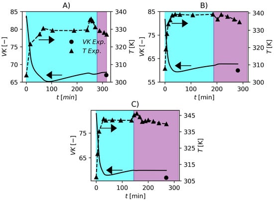
Figure 2.
Values of VK obtained experimentally and predicted by the proposed model. (A) F1, (B) F2 and (C) F3. Cyan and purple shadowed areas represent the ranges of and , respectively.
In Figure 2, the temperatures and of the three formulations are shown. In this case, the temperature data profiles were used as model inputs in the parameter estimation strategy since the model presented in this work does not contemplate an energy balance so far. The obtained fits of can be regarded as very satisfactory. As expected, it is possible to observe that the of the resin varies inversely with temperature which shows the model consistency once again. To conclude this section, Figure 3 shows a plot of suspension viscosity and surface tension for one the studied industrial grade formulations.
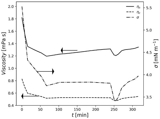
Figure 3.
Variation of suspension properties in F1.
4.2. Estimation of Breakage and Coalescence Parameters
In the present paper, two reactor types were considered. The formulation 1 (F1) was carried out in a reactor equipped with a reflux condenser on its top, while the second and third formulations (F2 and F3) were carried out in a reactor equipped only with a cooling jacket for temperature control. The top reflux condenser can significantly affect the particle nucleation mechanism (as a flow of cold monomer is continuously fed into the reactor) and the rates of breakage and coalescence inside the vessel. For instance, Cheng and Langsam [96] observed coarsening of the particle size distribution when the top reflux condenser was used. Moreover, these authors also found that the percentage of coarse particles was proportional to the reflux rate and this effect became negligible when the operation of the top reflux condenser was initiated after conversion of 30%, when the polymer particle approached the particle identification point, i.e., when droplet breakage and coalescence cease. Therefore, the parameter estimations were performed for each type of reactor independently. Two types of data were available for the present study: sieve tests and distributions obtained by laser scattering (Mastersizer 3000, Malvern Penalytical, Malvern, UK). More specifically, the sieve tests for the three formulations were available whereas the particle size distributions by laser scattering were available only for F1 and F2 (due to internal regulations, the laser scattering tests were about to be replaced by sieve tests). In order to perform the parameter estimation, the problem 58 was solved with the PSO algorithm [94,95] with the same parameters employed previously, except the search region, obviously. In Equation (58), represents the final cumulative particle size distribution. The estimated parameters were and in Equations (47) and (48).
The parameter sets PS1 and PS2 in Table 7 were estimated based on laser diffraction data provided by industrial runs F1 and F2. The obtained fits are shown in Figure 4. According to the figure, these two parameter sets can represent the available industrial data accurately, which illustrates the flexibility of the proposed modeling approach. Even though it is tempting to compare the estimated parameter sets with the values reported by Coulaloglou and Tavlarides [50], such a comparison may not be informative due to four main reasons. Firstly, in their original work, the authors represented the breakage, coalescence and daughter droplet distributions in terms of droplet volume, as discussed previously. Secondly, the vessel employed in their study had only 12 L, while the industrial vessels considered in the present work have tens of cubic meters. Thirdly, a different system was employed in their study (water-kerosene-dichlorobenzene). Lastly, these investigators worked with very dispersed systems, where ; so that was significantly smaller than the values used in the present work ()
Table 7.
Search region and estimated parameters in the breakage and coalescence rate equations.
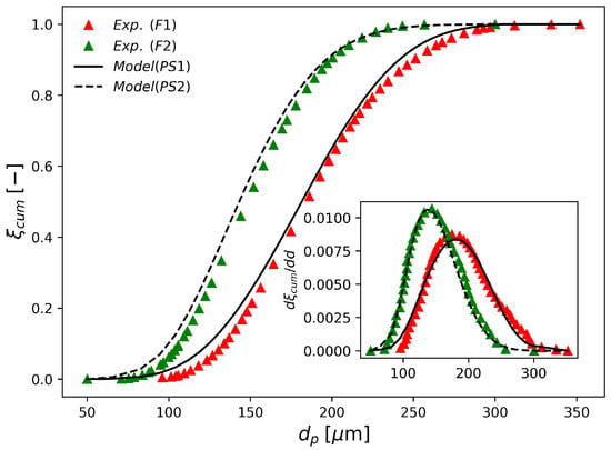
Figure 4.
Experimental and simulated final cumulative particle size distributions obtained with parameters shown in Table 7.
In spite of that, as and represent the frequencies of breakage and coalescence, respectively; and and represent the efficiencies of breakage and coalescence, respectively; it can be noticed that the breakage efficiencies in the two polymerization reactors are very similar. Additionally, the breakage frequency in the reactor equipped with a top reflux condenser is also very similar to its counterpart in the reactor without a top reflux condenser, which puts in evidence the fact that the breakage mechanism in both vessels is very similar. Moreover, just to put it into perspective, the breakage efficiency proposed by Coulaloglou and Tavlarides [50] is nearly four orders of magnitude greater than the breakage efficiencies in the industrial reactors (pay attention to the negative sings of the exponential terms in Equations (44) and (45)) whereas the breakage frequency is two orders of magnitude higher. This can be attributed to the small hold up in the smaller reactor, which favors breakage [50,51,55] and the fact that the smaller reactor is more homogeneous and have less stagnation zones. Furthermore, regarding the industrial reactors, the coalescence efficiency in the polymerization reactor with a top reflux condenser is smaller even tough the coalescence frequency is higher. This can be attributed to the effect of the top reflux condenser on the rates, as discussed previously. The coalescence efficiencies in the polymerization reactors are notably higher (6 orders of magnitude) than the efficiencies in the vessel from Coulaloglou and Tavlarides [50], which can be attributed to larger hold up and volume also discussed previously. The coalescence frequencies in the polymerization reactors are two orders of magnitude higher than that in the smaller vessel. To the best of our knowledge, this has never been discussed in the polymerization literature.
In Figure 5, the rate of droplet breakage for different hold up fractions and calculated with parameters PS1 is plotted against the droplet diameter at zero conversion. It can be seen that larger droplets are more prone to breakage, as expected. Additionally, as the hold up increases the breakage rate decreases which is a very known effect according to the literature [50,51,55]. In Figure 6, the coalescence rate calculated with parameters PS1 is shown. According to this set of parameters, the highest coalescence rates are obtained between large and small droplets. On the other hand, the smaller droplets are less likely to coalesce with other small droplets. Furthermore, as the hold up fraction increases, the coalescence rate of droplets of intermediate sizes also increases. The coalescence rate plotted is symmetrical around the secondary diagonal of the plot, as expected, since . As discussed in the development of the population balance model, the coalescence rates of droplets with masses and such that are zero because it would result in particles with masses outside the discretization range. This is the reason why the upper part of the plots are ignored.
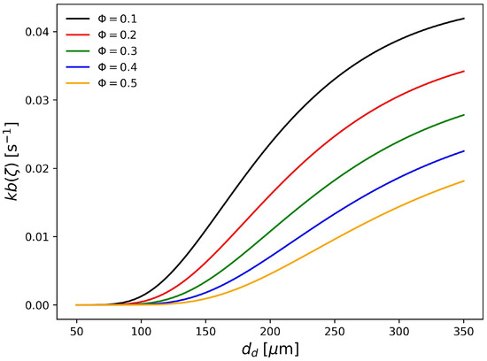
Figure 5.
Breakage rate (Pa s, kg m, N m) for different dispersed phase volume fraction calculated with parameter set PS1.
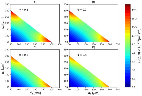
Figure 6.
Coalescence rate (Pa s, kg m, N m) for different dispersed phase volume fractions calculated with parameter set PS1. (A) , (B) , (C) and (D) .
In order to emphasize the difference in coalescence rates due to cold monomer refluxing, in Figure 7 the coalescence rate calculated with parameters PS2 is shown. In this case, a much more uniform profile is observed where the coalescence rate of large and small droplets is nearly the same of droplets of intermediate sizes. Based on the colorbars of the Figure 6 and Figure 7 it is possible to affirm that coalescence rate in the reactor with a top reflux condenser is roughly 5 times higher than its counterpart in the reactor without cold monomer refluxing.
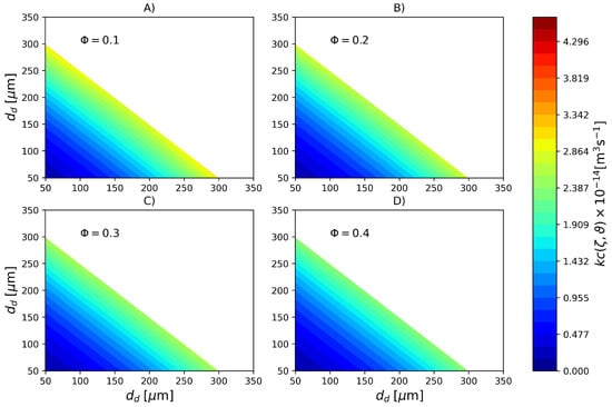
Figure 7.
Coalescence rate (Pa s, kg m, N m) for different dispersed phase volume fractions calculated with parameter set PS2. (A) , (B) , (C) and (D) .
In Figure 8, it is shown the experimental and predicted sieve data for the three formulations. Even though the parameters sets PS1 and PS2 were estimated with the laser diffraction data, these sets of parameters also represent the sieve data with remarkable accuracy, specially F1 and F3. The sieve data in F2 shows a slightly lower average than the model prediction, this can be attributed to additional breakage that occurs due to the shaking of the equipment during the test.
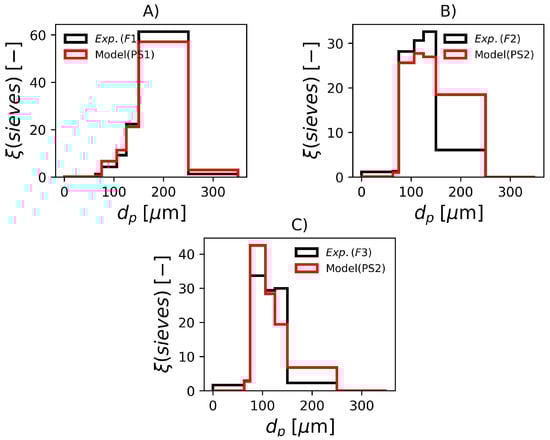
Figure 8.
Experimental and simulated sieve data with parameters in Table 7. (A) F1, (B) F2 and (C) F3.
4.3. Effect of Process Variables
To be useful at the plant site, the proposed model must be able to represent the effect of operation variables on the final product properties. For this reason, in the present section, the effect of perturbations on particle properties is investigated. According to Figure 9, when the rotation speed is reduced by 10%, is increased by about 11% in operation conditions F1. On the other hand, an increase of 10% in impeller rotation causes a decrease of 8.7% in . Regarding F2, increases 13.6% when the impeller speed drops by 10% and decreases by 10% when impeller rotation increases 10%. In the conditions studied, the magnitude of the change in impeller rotation causes similar changes in the particle mean diameter. However, since the formulations are different, i.e., different amounts of PVA, temperature, initiator and dispersed phase fraction, it becomes difficult to analyse the effect of the impeller speed on the rates solely. Additionally, the relationships between these variables in the rate equations is nonlinear. Consequently, in order to compare the rates and their effects on both reactors, it would be necessary that the same formulations were produced on each of them.
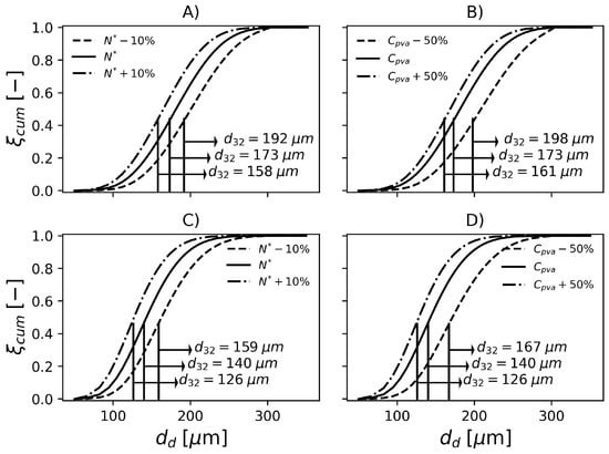
Figure 9.
Effect of impeller rotation and PVA concentration on particle size distribution in F1, (A) and (B), respectively. Effect of impeller rotation and PVA concentration on particle size distribution in F2, (C) and (D), respectively.
The model predictions appear to be less sensitive to changes in PVA concentration. Still regarding Figure 9, decreasing the PVA concentration by causes a 14.4% increase in in F1. Additionally, an increase of 50% causes a 7% decrease in . With respect to F2, the 50% decrease in PVA causes 19.3% increase in and an increase of 50% causes 10% decrease in . The influence of PVA concentration might be underestimated/overestimated because the model does not consider the degree of hydrolysis in the equation that represents the surface tension (), see Table 3.
4.4. Evolution of Mean Particle and Droplet Diameters
In Figure 10 and Figure 11, it is shown the evolution of droplet and particle mean diameters for the conditions studied in the previous section. Additionally, the results are compared with those obtained with conditions F1 and F2. Regarding Figure 10, the beginning of the reaction is marked by strong droplet coalescence. Then the breakage mechanism becomes predominant until 30% conversion. The transition from pink to cyan in these figures, marks the point where the 30% conversion is surpassed. At this point, the polymerizing monomer droplets become rigid and are not prone to breakage and coalescence according to the present model. It is possible to notice a decrease in droplet diameter as conversion advances. In fact, this is a consequence of the increasing droplet density, as the fraction of polymer increases and the density of PVC is higher than that of VCM. This shrinking phenomena continues until the end of the reaction when .
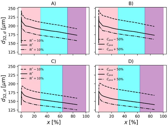
Figure 10.
Evolution of Sauter mean diameter of the droplets. Effect of impeller rotation and PVA concentration in F1, (A) and (B), respectively. Effect of impeller rotation and PVA concentration in F2, (C) and (D), respectively. Pink, cyan and purple shadowed areas represent the ranges of conversion , and , respectively.
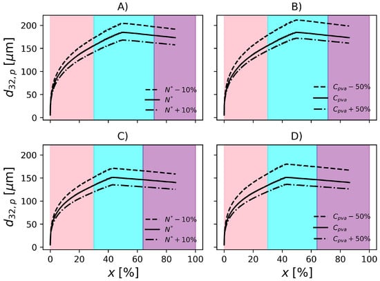
Figure 11.
Evolution of Sauter mean diameter of the particles. Effect of impeller rotation and PVA concentration in F1, (A) and (B), respectively. Effect of impeller rotation and PVA concentration in F2, (C) and (D), respectively. Pink, cyan and purple shadowed areas represent the ranges of conversion , and , respectively.
In Figure 11, it is possible to observe that the particle size increases with conversion, as expected, due agglomeration of primary particles to form the agglomerates, in accordance with Xie et al. [36] and Cebollada et al. [97]. The slight decrease is a consequence of the decrease in particle porosity as monomer is consumed and the particle becomes denser.
5. Conclusions
In the present paper, a model was built and implemented to represent the trajectories of mass inventories, pressures and polymer properties, with emphasis on the final particle size distributions in industrial scale PVC suspension polymerization reactors for the first time. It was shown that after proper parameter estimation, the model is able to represent the operation of industrial scale reactors and describe the final particle size distributions, as measured through sieve tests and laser scattering analyses. Even tough turbulence homogeneity was assumed in the entire vessel, the obtained model predictions can be regarded as very good. Particularly, it was shown for the first time that the frequency and efficiency of breakage in the reactor equipped with a top reflux condenser were very similar to their counterparts in the reactor without a reflux condenser. However, the coalescence frequency was larger in the reactor with a top reflux condenser, which emphasizes that refluxing cold monomer to the vessel favors coalescence and tends to result in larger particles.
Author Contributions
Conceptualization, J.d.S.S., P.A.M. and J.C.P.; methodology, J.d.S.S., P.A.M. and J.C.P.; software, J.d.S.S. and J.C.P.; validation, J.d.S.S., P.A.M. and J.C.P.; formal analysis, J.d.S.S.; investigation, J.d.S.S. and J.C.P.; data curation, J.d.S.S.; writing—original draft preparation, J.d.S.S.; writing—review and editing, P.A.M. and J.C.P.; visualization, J.d.S.S.; supervision, J.C.P.; project administration, J.C.P.; funding acquisition, J.C.P. All authors have read and agreed to the published version of the manuscript.
Funding
This study was financed in part by the Coordenação de Aperfeiçoamento de Pessoal de Nível Superior—Brasil (CAPES)—Finance Code 001.
Data Availability Statement
Not applicable.
Acknowledgments
The authors thank CAPES (Coordenação de Aperfeiçoamento de Pessoal de Nível Superior, Brazil, Finance Code 001) and CNPq (Conselho Nacional de Desenvolvimento Científico e Tecnológico, Brazil).
Conflicts of Interest
The authors declare no conflict of interest.
Abbreviations
The following abbreviations are used in this manuscript:
| CAGR | Compound Annual Growth Rate |
| CFD | Computational Fluid Dynamics |
| CLD | Chain Length Distribution |
| MMA | Methyl Methacrylate |
| MMD | Molar Mass Distribution |
| PE | Poly(ethylene) |
| PMMA | Poly(methyl methacrylate) |
| PP | Poly(propylene) |
| PVA | Poly(vinyl alcohol) |
| PVC | Poly(vinyl chloride) |
| PSO | Particle Swarm Optimization |
| VCM | Vinyl Chloride Monomer |
List of Symbols
The following symbols are used in this manuscript:
| A | Free volume parameter used in equation [-] |
| B | Free volume parameter used in equation [-] |
| Free volume parameter used in equation [-] | |
| C | Free volume parameter used in equation [-] |
| Empirical constants [-] | |
| PVA concentration [kg m] | |
| Particle diameter [m] | |
| Droplet diameter [m] | |
| Sauter mean diameter [m] | |
| Activation energies in the free volume parameters [K] | |
| f | Initiator efficiency [-] |
| I | Initiator [kmol] |
| Monomer solubility [kg kg] | |
| Initiator partition coefficient [-] | |
| Coalescence rate [m s] | |
| Breakage rate [s] | |
| Propagation rate constant [m kmol s] | |
| Initiator decomposition rate constant [s] | |
| Transfer to monomer rate constant [m kmol s] | |
| Termination rate constant [m kmol s] | |
| Termination by combination rate constant [m kmol s] | |
| Termination by disproportionation rate constant [m kmol s] | |
| L | Impeller diameter [m] |
| m | Monomer [kg] |
| M | Monomer [kmol] |
| Molar mass [kg kmol] | |
| Number average molar mass [kg kmol] | |
| Weight average molar mass [kg kmol] | |
| Number of initiators [-] | |
| Number of mass classes [-] | |
| N | Number of droplets [-] |
| Impeller rotation speed [hz] | |
| p | Polymer [kg] |
| P | Polymer [kmol] |
| R | Ideal gas constant [m Pa kmol K] |
| t | Time [s] |
| T | Temperature [K] |
| Glass transition temperature [K] | |
| V | Volume [m] |
| Suspension volume [m] | |
| K Value [-] | |
| Free volume at [-] | |
| x | Conversion [-] |
| Critical conversion [-] | |
| y | Volume fraction [-] |
| w | Water [kg] |
| Z | Pressure [Pa] |
| Subscripts | |
| j | Relative to phase j |
| 1 | Relative to phase 1 (monomer-rich) |
| 2 | Relative to phase 2 (polymer-rich) |
| 3 | Relative to phase 3 (aqueous phase) |
| 4 | Relative to phase 4 (gaseous phase) |
| m | Monomer |
| p | Polymer |
| w | Water |
| s | Suspension |
| d | Dispersed phase |
| c | Continuous phase |
| t | Total |
| k | Initiator type () |
| Greek symbols | |
| Porosity [-] | |
| order living polymer moment [kmol] | |
| order dead polymer moment [kmol] | |
| Polymer volume fraction in phase 2 [-] | |
| Dispersed phase volume fraction [-] | |
| Flory-Huggins interaction parameter [-] | |
| Viscosity [Pa s] | |
| Intrinsic viscosity [m kg] | |
| Density [kg m] | |
| Daughter droplet distribution [-] | |
| Droplet mass [kg] | |
| Surface tension [N m] | |
| Variance [kg] | |
| Total mass of particles of mass i [kg] |
References
- Guo, Y.; Leroux, F.; Tian, W.; Li, D.; Tang, P.; Feng, Y. Layered double hydroxides as thermal stabilizers for poly(vinyl chloride): A review. Appl. Clay Sci. 2021, 211, 106198. [Google Scholar] [CrossRef]
- Precedence Research. Available online: https://www.precedenceresearch.com/pvc-pipes-market (accessed on 7 February 2023).
- Kanking, S.; Pulngern, T.; Rosarpitak, V.; Sombatsompop, N. Temperature profiles and electric energy consumption for wood/Poly(vinyl chloride) composite and fibre cement board houses. J. Build. Eng. 2021, 42, 102784. [Google Scholar] [CrossRef]
- Kwon, C.W.; Chang, P. Influence of alkyl chain length on the action of acetylated monoglycerides as plasticizers for poly (vinyl chloride) food packaging film. Food Packag. Shelf Life 2021, 27, 100619. [Google Scholar] [CrossRef]
- Ekelund, M.; Edin, H.; Gedde, U.W. Long-term performance of poly(vinyl chloride) cables Part 1: Mechanical and Electrical Performances. Polym. Degrad. Stab. 2007, 92, 617–629. [Google Scholar] [CrossRef]
- Islam, I.; Sultana, S.; Ray, S.W.; Nur, H.P.; Hossain, M.T.; Ajmotgir, W.M. Electrical and tensile properties of carbon black reinforced polyvinyl chloride conductive composites. C 2018, 4, 15. [Google Scholar] [CrossRef]
- Hakkarainen, M. New PVC materials for medical applications—The release profile of PVC/polycaprolactone-polycarbonate aged in aqueous environments. Polym. Degrad. Stab. 2003, 80, 451–458. [Google Scholar] [CrossRef]
- Chiellini, F.; Ferri, M.; Morelli, A.; Dipaola, L.; Latini, G. Perspectives on alternatives to phthalate plasticized poly(vinyl chloride) in medical devices applications. Prog. Polym. Sci. 2013, 38, 1067–1088. [Google Scholar] [CrossRef]
- Mijangos, C.; Calafel, I.; Santamaría, A. Poly(vinyl chloride), a historical polymer still evolving. Polymer 2023, 266, 125610. [Google Scholar] [CrossRef]
- Abreu, C.M.R.; Fonseca, A.C.; Rocha, N.M.P.; Guthrie, J.T.; Serra, A.C.; Coelho, J.F.J. Poly(vinyl chloride): Current status and future perspectives via reversible deactivation radical polymerization methods. Prog. Polym. Sci. 2018, 87, 34–69. [Google Scholar] [CrossRef]
- Kiparissides, C.; Pladis, P. On the prediction of suspension viscosity, grain morphology, and agitation power in SPVC reactors. Can. J. Chem. Eng. 2022, 100, 714–730. [Google Scholar] [CrossRef]
- Yuan, H.G.; Kalfas, G.; Ray, W.H. Suspension Polymerization. J. Macromol. Sci. Rev. Macromol. Chem. Phys. 1991, C31, 215–299. [Google Scholar] [CrossRef]
- Machado, F.; Lima, E.L.; Pinto, J.C. A review on suspension polymerization processes. Polimeros 2007, 17, 166–179. [Google Scholar] [CrossRef]
- Pinto, M.C.C.; Santos, J.G.F., Jr.; Machado, F.; Pinto, J.C. Suspension polymerization processes. In Encyclopedia of Polymer Science and Technology; Wiley: Hoboken, NJ, USA, 2013. [Google Scholar]
- Crosato-Arnaldi, A.; Gasparini, P.; Talamini, G. The bulk and suspension polymerization of vinyl chloride. Die Makromol. Chem. 1968, 117, 140–152. [Google Scholar] [CrossRef]
- Guo, R.; Yu, E.; Liu, J.; Wei, Z. Agitation transformation during vinyl chloride suspension polymerization: Aggregation morphology and PVC properties. RSC Adv. 2017, 7, 24022. [Google Scholar] [CrossRef]
- Marinho, R.; Horiuchi, L.; Pires, C.A. Effect of stirring speed on conversion and time to particle stabilization of poly(vinyl chloride) produced by suspension polymerization process at the beginning of reaction. Braz. J. Chem. Eng. 2018, 35, 631–640. [Google Scholar] [CrossRef]
- Chatzi, E.G.; Kiparissides, C. Drop size distribution in high holdup fraction dispersion systems: Effect of the degree of hydrolysis of PVA stabilizer. Chem. Eng. Sci. 1994, 49, 5039–5052. [Google Scholar] [CrossRef]
- Lerner, F.; Nemet, S. Effects of poly(vinyl acetate) suspending agents on suspension polymerisation of vinyl chloride monomer. Plast. Rubber Compos. 1999, 28, 100–104. [Google Scholar] [CrossRef]
- Kiparissides, C. Polymerization reactor modeling: A review of recent developments and future directions. Chem. Eng. Sci. 1996, 51, 1637–1659. [Google Scholar] [CrossRef]
- Darvish, R.; Esfahany, M.N.; Bagheri, R. S-PVC grain morphology: A review. Ind. Eng. Chem. Res. 2015, 54, 10953–10963. [Google Scholar] [CrossRef]
- Faria, J.M., Jr.; Lima, E.L.; Pinto, J.C.; Machado, F. Monitoramento in situ e em tempo real de variáveis morfológicas do poli(cloreto de vinila) usando espectroscopia NIR. Polímeros 2009, 19, 95–104. [Google Scholar] [CrossRef]
- Faria, J.M., Jr.; Machado, F.; Lima, E.L.; Pinto, J.C. Monitoring of vinyl chloride suspension polymerization using NIRS 1. prediction of morphological properties. Comput.-Aided Chem. Eng. 2009, 27, 327–332. [Google Scholar]
- Faria, J.M., Jr.; Machado, F.; Lima, E.L.; Pinto, J.C. Monitoring of vinyl chloride suspension polymerization using NIRS 2. proposition of a scheme to control morphological properties. Comput.-Aided Chem. Eng. 2009, 27, 1329–1334. [Google Scholar]
- Faria Jr, J.M.; Machado, F.; Lima, E.L.; Pinto, J.C. In-line monitoring of vinyl chloride suspension polymerization with near infrared spectroscopy, 1—Analysis of morphological properties. Macromol. React. Eng. 2010, 4, 11–24. [Google Scholar]
- Faria, J.M., Jr.; Machado, F.; Lima, E.L.; Pinto, J.C. In-line monitoring of vinyl chloride suspension polymerization with near infrared spectroscopy, 2—Design of an advanced control strategy. Macromol. React. Eng. 2010, 4, 486–498. [Google Scholar]
- Talamini, G. The heterogeneous bulk polymerization of vinyl chloride. J. Polym. Sci. 1966, 4, 535–537. [Google Scholar]
- Abdel-Alim, A.H.; Hamielec, A.E. Bulk polymerization of vinyl chloride. J. Appl. Polym. Sci. 1972, 16, 783–799. [Google Scholar] [CrossRef]
- Ugelstad, J.; Flogstad, H.; Hertzberg, T.; Sund, E. On the bulk polymerization of vinyl chloride. Die Makromoleckulare Chem. 1973, 164, 171–181. [Google Scholar] [CrossRef]
- Kuchanov, S.I.; Bort, D.N. Kinetics and mechanism of bulk polymerization of vinyl chloride. Vysokomol. Soyed. 1973, A15, 2393–2412. [Google Scholar] [CrossRef]
- Hamielec, A.E.; Gomez-Vaillard, R.; Marten, F.L. Diffusion-controlled free radical polymerization. effect on polymerization rate and molecular properties of polyvinyl chloride. J. Macromol. Sci. Part A Pure Appl. Chem. 1982, A17, 1005–1020. [Google Scholar] [CrossRef]
- Sidiropoulou, E.; Kiparissides, C. The title of the cited article. J. Macromol. Sci. Part A Pure Appl. Chem. 1990, 27, 257–288. [Google Scholar] [CrossRef]
- Pinto, J.C. Vinyl chloride suspension polymerization with constant rate. a numerical study of batch reactors. J. Vinyl Tech. 1990, 12, 7–12. [Google Scholar] [CrossRef]
- Pinto, J.C. Dynamic behavior of continuous vinyl chloride bulk and suspension polymerization reactors. a simple model analysis. Polym. Eng. Sci. 1990, 30, 291–302. [Google Scholar] [CrossRef]
- Pinto, J.C. Dynamic Behavior of Continuous Vinyl Chloride Suspension Polymerization Reactors: Effects of Segregation. Polym. Eng. Sci. 1990, 30, 925–930. [Google Scholar] [CrossRef]
- Xie, T.Y.; Hamielec, A.E.; Wood, P.E.; Woods, D.R. Experimental investigation of vinyl chloride polymerization at high conversion: Mechanism, kinetics and modelling. Polymer 1991, 32, 537–557. [Google Scholar] [CrossRef]
- Xie, T.Y.; Hamielec, A.E.; Wood, P.E.; Woods, D.R. Experimental investigation of vinyl chloride polymerization at high conversion—Reactor dynamics. J. Appl. Polym. Sci. 1991, 43, 1259–1269. [Google Scholar] [CrossRef]
- Xie, T.Y.; Hamielec, A.E.; Wood, P.E.; Woods, D.R. Experimental investigation of vinyl chloride polymerization at high conversion: Semi-batch reactor modelling. Polymer 1991, 32, 2087–2095. [Google Scholar] [CrossRef]
- Xie, T.Y.; Hamielec, A.E.; Wood, P.E.; Woods, D.R. Experimental investigation of vinyl chloride polymerization at high conversion: Molecular-weight development. Polymer 1991, 32, 1098–1111. [Google Scholar] [CrossRef]
- Xie, T.Y.; Hamielec, A.E.; Wood, P.E.; Woods, D.R. Suspension, bulk, and emulsion polymerization of vinyl chloride—Mechanism, kinetics, and reactor modelling. J. Vinyl Tech. 1991, 13, 2–25. [Google Scholar] [CrossRef]
- Dimian, A.; van Diepen, D.; van der Wal, G.A. Dynamic simulation of a PVC suspension reactor. Comput. Chem. Eng. 1995, 19, 427–432. [Google Scholar] [CrossRef]
- Chung, S.T.; Jung, S.H. Kinetic modeling of commercial scale mass polymerization of vinyl chloride. J. Vinyl Add. Tech. 1996, 2, 295–303. [Google Scholar] [CrossRef]
- Lewin, D.R. Modelling and control of an industrial PVC suspension polymerization reactor. Comput. Chem. Eng. 1996, 20, S865–S870. [Google Scholar] [CrossRef]
- Kiparissides, C.; Daskalakis, G.; Achilias, D.S.; Sidiropoulou, E. Dynamic simulation of industrial poly(vinyl chloride) batch suspension polymerization reactors. Ind. Eng. Chem. Res. 1997, 36, 1253–1267. [Google Scholar] [CrossRef]
- Talamini, G.; Visentini, A.; Kerr, J. Bulk and suspension polymerization of vinyl chloride: The two-phase model. Polymer 1998, 39, 1879–1891. [Google Scholar] [CrossRef]
- Mejdell, T.; Pettersen, T.; Naustdal, C.; Svendsen, H.F. Modelling of industrial S-PVC reactor. Chem. Eng. Sci. 1999, 54, 2459–2466. [Google Scholar] [CrossRef]
- Wieme, J.; De Roo, T.; Marin, G.B.; Heynderickx, G.J. Simulation of pilot- and industrial-scale vinyl chloride batch suspension polymerization reactors. Ind. Eng. Chem. Res. 2007, 46, 1179–1196. [Google Scholar] [CrossRef]
- Valentas, K.J.; Bilous, O.; Amundson, N.R. Analysis of breakage in dispersed phase systems. Ind. Eng. Chem. Fundamen. 1966, 5, 271–279. [Google Scholar] [CrossRef]
- Valentas, K.J.; Amundson, N.R. Breakage and coalescence in dispersed phase systems. Ind. Eng. Chem. Fundamen. 1966, 5, 533–542. [Google Scholar] [CrossRef]
- Coulaloglou, C.A.; Tavlarides, L.L. Description of interaction processes in agitated liquid-liquid dispersions. Chem. Eng. Sci. 1977, 32, 1289–1297. [Google Scholar] [CrossRef]
- Narsimhan, G.; Gupta, J.P.; Ramkrishna, D. A model for transitional breakage probability of droplets in agitated lean liquid-liquid dispersions. Chem. Eng. Sci. 1979, 34, 257–265. [Google Scholar] [CrossRef]
- Hsia, M.A.; Tavlarides, L.L. A simulation model for homogeneous dispersions in stirred tanks. Chem. Eng. J. 1980, 20, 225–236. [Google Scholar] [CrossRef]
- Hsia, M.A.; Tavlarides, L.L. Simulation analysis of drop breakage, coalescence and micromixing in liquid-liquid stirred tanks. Chem. Eng. J. 1983, 26, 189–199. [Google Scholar] [CrossRef]
- Sovová, H. Breakage and coalescence of drops in a batch stirred vessel-II comparison of model and experiments. Chem. Eng. Sci. 1981, 36, 1567–1573. [Google Scholar] [CrossRef]
- Alvarez, J.; Alvarez, J.; Hernández, M. A population balance approach for the description of particle size distribution in suspension polymerization reactors. Chem. Eng. Sci. 1994, 49, 99–113. [Google Scholar] [CrossRef]
- Maggioris, D.; Goulas, A.; Alexopoulos, A.H.; Chatzi, E.G.; Kiparissides, C. Prediction of particle size distribution in suspension polymerization reactors: Effect of turbulence nonhomogeneity. Chem. Eng. Sci. 2000, 55, 4611–4627. [Google Scholar] [CrossRef]
- Kotoulas, C.; Kiparissides, C. A generalized population balance model for the prediction of particle size distribution in suspension polymerization reactors. Chem. Eng. Sci. 2006, 61, 332–346. [Google Scholar] [CrossRef]
- Machado, R.A.F.; Pinto, J.C.; Araújo, P.H.H.; Bolzan, A. Mathematical modeling of polystyrene particle size distribution produced by suspension polymerization. Braz. J. Chem. Eng. 2000, 17, 4–7. [Google Scholar] [CrossRef]
- Kiparissides, C.; Alexopoulos, A.; Roussos, A.; Dompaziz, G.; Kotoulas, C. Population balance modeling of particulate polymerization processes. Ind. Eng. Chem. Res. 2004, 43, 7290–7302. [Google Scholar] [CrossRef]
- Kiparissides, C. Challenges in particulate polymerization reactor modeling and optimization: A population balance perspective. J. Process Control 2006, 16, 205–224. [Google Scholar] [CrossRef]
- Alexopoulos, A.H.; Kiparissides, C. On the prediction of internal particle morphology in suspension polymerization of vinyl chloride. Part I: The effect of primary particle size distribution. Chem. Eng. Sci. 2007, 62, 3970–3983. [Google Scholar] [CrossRef]
- Bárkányi, A.; Németh, S.; Lakatos, B.G. Modeling and simulation of suspension polymerization of vinyl chloride via population balance model. Comput. Chem. Eng. 2013, 59, 211–218. [Google Scholar] [CrossRef]
- Kiparissides, C. Modeling of suspension vinyl chloride polymerization: From kinetics to particle size distribution and PVC grain morphology. Adv. Polym. Sci. 2018, 280, 121–194. [Google Scholar]
- Koolivand, A.; Shahrokhi, M.; Farahzadi, H. Optimal control of molecular weight and particle size distributions in a batch suspension polymerization reactor. Iran. Polym. J. 2019, 28, 735–745. [Google Scholar] [CrossRef]
- Kim, S.H.; Lee, J.H.; Braatz, R.D. Multi-scale fluid dynamics simulation based on MP-PIC-PBE method for PMMA suspension polymerization. Comput. Chem. Eng. 2021, 152, 107391. [Google Scholar] [CrossRef]
- Alexopoulos, A.H.; Maggioris, D.; Kiparissides, C. CFD analysis of turbulence non-homogeneity in mixing vessels a two-compartment model. Chem. Eng. Sci. 2002, 57, 1735–1752. [Google Scholar] [CrossRef]
- Burgess, R.H. Suspension polymerization of vinyl chloride. In Manufacturing and Processing of PVC; Burgess, R.H., Ed.; Elsevier: Barking, UK, 1982; pp. 1–27. [Google Scholar]
- Park, G.S.; Smith, D.G. Vinyl chloride studies. II. initiation and termination in the homogeneous polymerization of vinyl chloride. Die Makromol. Chem. 1970, 131, 1–6. [Google Scholar] [CrossRef]
- Bachmann, R.; Melchiors, M.; Avtomonov, E. Modelling and optimization of nonlinear polymerization processes. Macromol. Symp. 2016, 370, 135–143. [Google Scholar] [CrossRef]
- Mastan, E.; Zhu, S. Method of moments: A versatile tool for deterministic modeling of polymerization kinetics. Eur. Polym. J. 2015, 68, 139–160. [Google Scholar] [CrossRef]
- Silva, J.S. Modeling and Experimental Investigation of Continuous Suspension Polymerization Processes. PhD Qualifying Examination, Universidade Federal do Rio de Janeiro, Rio de Janeiro, Brazil, 2020. [Google Scholar]
- Bueche, F. Physical Properties of Polymers; Interscience Publishers: New York, NY, USA, 1962; pp. 112–120. [Google Scholar]
- Fedors, R.F. A universal reduced glass transition temperature for liquids. J. Polym. Sci. 1979, 17, 719–722. [Google Scholar] [CrossRef]
- Reding, F.P.; Walter, E.R.; Welch, F.J. Glass transition and melting point of poly(vinyl chloride). J. Polym. Sci. 1962, 56, 225–231. [Google Scholar] [CrossRef]
- Ceccorulli, G.; Pizzoli, M.; Pezzin, G. Effect of thermal history on Tg and corresponding CP changes in PVC of different stereoregularities. J. Macromol. Sci. Part B Phys. 1977, 14, 499–510. [Google Scholar] [CrossRef]
- Burnett, G.M.; Wright, W.W. The photosensitized polymerization of vinyl chloride in tetrahydrofuran solution. III. determination of the kinetic coefficients. Proc. R. Soc. Lond. A 1954, 221, 41–53. [Google Scholar]
- Si, K. Kinetics and Mechanism of Vinyl Chloride Polymerization: Effects of additives on Polymerization Rate, Molecular Weight and Defect Concentration in the Polymer. Doctoral Dissertation, Case Western Reserve University, Cleveland, OH, USA, May 2007. [Google Scholar]
- Skillicorn, D.E.; Perkins, G.G.A.; Slark, A.; Dawkins, J.V. Molecular weight and solution viscosity characterization of PVC. J. Vinyl Tech. 1993, 15, 105–108. [Google Scholar] [CrossRef]
- Nilsson, H.; Silvergren, C.; Tornell, B. Suspension stabilizers for PVC production I: Interfacial tension measurements. J. Vinyl Tech. 1985, 7, 112–118. [Google Scholar] [CrossRef]
- Lazrak, N.; Le Bolay, N.; Ricard, A. Droplet stabilization in high holdup fraction suspension polymerization reactors. Eur. Polym. J. 1998, 34, 1637–1647. [Google Scholar] [CrossRef]
- Korosi, A.; Fabuss, B.M. Viscosity of liquid water from 25o to 150o. measurements in pressurized glass capillary viscometer. Anal. Chem. 1968, 40, 157–162. [Google Scholar] [CrossRef]
- Perry, R.H.; Green, D.W. Perry’s Chemical Engineers’ Handbook, 8th ed.; McGraw Hill: New York, NY, USA, 2008. [Google Scholar]
- Okaya, T. Modification of Polyvinyl Alcohol by Copolymerization. In Polyvinyl Alcohol Developments; Finch, C.A., Ed.; Wiley: Hoboken, NJ, USA, 1992. [Google Scholar]
- Batchelor, G.; Green, J. The hydrodynamic interaction of two small freely-moving spheres in a linear flow field. J. Fluid Mech. 1972, 56, 375–400. [Google Scholar] [CrossRef]
- Nagy, D.J. A Mark-Houwink equation for poly(vinyl alcohol) from sec-viscometry. J. Liq. Chromatogr. 1993, 16, 3041–3058. [Google Scholar] [CrossRef]
- Vermeulen, T.; Williams, G.M.; Langlois, G.E. Interfacial area in liquid-liquid and gas-liquid agitation. Chem. Eng. Prog. 1955, 51, 85F–95F. [Google Scholar]
- Bouyatiotis, B.A.; Thornton, J.D. Liquid-liquid extraction studies in stirred tanks. part I. droplet size and hold-up measurements in a seven-inch diameter baffled vessel. Inst. Chem. Eng. Symp. Series 1967, 26, 43–50. [Google Scholar]
- Nilsson, H.; Silvergreen, C.; Törnell, B. Swelling of PVC latex particles by VCM. Eur. Polym. J. 1978, 14, 737–741. [Google Scholar] [CrossRef]
- Solsvik, J.; Jakobsen, H.A. The foundation of the population balance equation: A review. J. Dispersion Sci. Technol. 2015, 36, 510–520. [Google Scholar] [CrossRef]
- Mikos, A.G.; Takoudis, C.G.; Peppas, N.A. Reaction engineering aspects of suspension polymerization. J. Appl. Polym. Sci. 1986, 31, 2647–2659. [Google Scholar] [CrossRef]
- Smallwood, P.V. The formation of grains of suspension poly(vinyl chloride). Polymer 1986, 27, 1609–1618. [Google Scholar] [CrossRef]
- Máriási, B. On the particle formation mechanism of poly(vinyl chloride)(PVC) powder produced by suspension polymerization-development of external morphology of particles. J. Vinyl Tech. 1986, 8, 20–26. [Google Scholar] [CrossRef]
- Petzold, L.R. Description of DASSL: A differential/Algebraic System Solver; Sandia National Labs.: Livermore, CA, USA, 1982. [Google Scholar]
- Kennedy, J.; Eberhart, R. Particle Swarm Optimization. Proc. IEEE Int. Conf. Neural Net. 1995, 4, 1942–1948. [Google Scholar]
- Schwaab, M.; Biscaia, E.C.; Monteiro, J.L.; Pinto, J.C. Nonlinear parameter estimation through particle swarm optimization. Chem. Eng. Sci. 2008, 63, 1542–1552. [Google Scholar] [CrossRef]
- Cheng, J.T.; Langsam, M. Particle structure of PVC based on cellulosic suspension system. III. effect of monomer refluxing. J. Appl. Polym. Sci. 1985, 30, 1365–1378. [Google Scholar] [CrossRef]
- Cebollada, A.F.; Schmidt, M.J.; Farber, J.N.; Capiati, N.J.; Vallés, E.M. Suspension Polymerization of Vinyl Chloride. I. Influence of Viscosity of Suspension Medium on Resin Properties. J. Appl. Polym. Sci. 1989, 37, 145–166. [Google Scholar] [CrossRef]


Disclaimer/Publisher’s Note: The statements, opinions and data contained in all publications are solely those of the individual author(s) and contributor(s) and not of MDPI and/or the editor(s). MDPI and/or the editor(s) disclaim responsibility for any injury to people or property resulting from any ideas, methods, instructions or products referred to in the content. |
© 2023 by the authors. Licensee MDPI, Basel, Switzerland. This article is an open access article distributed under the terms and conditions of the Creative Commons Attribution (CC BY) license (https://creativecommons.org/licenses/by/4.0/).