Process Simulation of Power-to-X Systems—Modeling and Simulation of Biological Methanation

Abstract

Through utilization of state-of-the-art power-to-x technology, biological methanation is a novel method to capture the intermittent electricity generated by renewable energy sources. In this process, biomass grows in a liquid solution by consuming H₂ and CO₂ and produces CH₄. This study aims to improve the accuracy and comprehensibility of an initial bio-methanation model by reviewing and comparing existing technologies and methods, correcting miswritten equations, adding complementary equations, and introducing a new initialization approach. In addition, a mean value approach was used for calculating the axial mixing coefficients. Gas–liquid mass transfer in the reactor, along with other aspects, is considered the most challenging aspect of the biological methanation process due to hydrogen’s low solubility. This highlights the need for a modeling approach to improve understanding and optimize the design of the process. The improved MATLAB code was used to test different variations of parameters in the reactor and observe their effects on the system’s performance. The model was validated using experimental cases, and the results indicate that it is more accurate than Inkeri’s for certain parameter variations. Moreover, it demonstrates better accuracy in depicting the pressure effect. The sensitivity analysis revealed that liquid recycle constant λ had little effect on methane concentration, while impeller diameter d_im and reactor diameter d_re had significant impacts. Axial mixing constants b₁ and b₂ and biological kinetics constants k_D, µ^max, and m_X had relatively small effects. Overall, the study presents a more comprehensive bio-methanation model that could be used to improve the performance of industrial reactors.

1. Introduction

Growing environmental concerns drive research on efficient, green technology such as clean fuels. Diverging prices for fossil fuels and renewables impact social and environmental outcomes. Renewable energy is crucial for reducing emissions, mitigating extreme weather, and ensuring reliable energy delivery [1]. To tackle variations in renewable electricity production, power-to-gas (PtG) systems convert excess electricity into methane (${\mathrm{CH}}_4$), a ${\mathrm{CO}}_2$-neutral fuel with higher energy density than hydrogen (${\mathrm{H}}_2$). Replacing gasoline with methane for generating 50 MJ of heat would result in 807 g less ${\mathrm{CO}}_2$ emissions.

1.1. Fundamentals of Biological Methanation

Methanation can either happen chemically or biologically. The first one is also referred to as the Sabatier process, which is represented by Equations (1) and (2), describing that hydrogen either reacts with carbon dioxide or carbon monoxide to produce methane and water, respectively [2,3]. Equation (1) is also valid for bio-methanation.

$$4{\mathrm{H}}_2+{\mathrm{CO}}_2\to {\mathrm{CH}}_4+2{\mathrm{H}}_2\mathrm{O}\hspace{1em}\Delta {\mathrm{H}}_{\mathrm{R}}=-165\mathrm{kJ}/\mathrm{mol}$$

(1)

$$3{\mathrm{H}}_2+\mathrm{CO}\to {\mathrm{CH}}_4+{\mathrm{H}}_2\mathrm{O}\hspace{1em}\hspace{1em}\Delta {\mathrm{H}}_{\mathrm{R}}=-206\mathrm{kJ}/\mathrm{mol}$$

(2)

An innovative PtG technique is electrolyzing water with excess energy to produce ${\mathrm{H}}_2$, which reacts with ${\mathrm{CO}}_2$ to yield ${\mathrm{CH}}_4$ in a process known as biological methanation (BM). BM is facilitated by special microorganisms called hydrogenotrophic methanogens from the Archaea domain. Unlike chemical methanation, biological methanation occurs at lower temperatures (−5 to 122 °C) [4,5] as opposed to 250–400 °C [6] and is more resistant to contaminants such as ${\mathrm{H}}_2\mathrm{S}$, organic acids, and ${\mathrm{NH}}_4{}^{+}$ [7]. Additionally, BM boasts a high ${\mathrm{CO}}_2$ to ${\mathrm{CH}}_4$ conversion ratio (around 95%) [8], tolerance against environmental perturbations in the field [9], and the potential to achieve energy independence and security through small decentralized biological methane manufacturing units integrated with renewable electricity generation sites [10]. The most critical and limiting factor in the bio-methanation process, specifically for ${\mathrm{H}}_2$, is gas–liquid mass transfer due to its low solubility [8,11,12,13,14,15]. Methanogens can only use hydrogen and carbon dioxide at the rate they are provided in the biomass culture. Increasing transfer surface area, such as in trickling bed and hollow fiber membrane reactors with packing, or extending retention times, can enhance hydrogen solubility [7]. Mechanical mixing in a continuously stirred tank reactor (CSTR) is a straightforward method for hydrogen dissolution [3].

Bio-methanation can occur either in situ, inside the anaerobic digester in the biogas plant, or ex situ, in a separate reactor specifically designed for hydrogenotrophic methanogens archaea [16]. Ex situ conditions provide an exclusive environment for the intended microorganisms and reactants, allowing for easier access and greater flexibility in measuring, modifying, and investigating various operating conditions and parameters in the reactor. Two temperature ranges are commonly used for anaerobic digestion and hydrogenotrophic methanogenesis: 55–65 °C for thermophilic and 35–40 °C for mesophilic archaea, each with different reaction rates. Temperature also affects physical properties involved in the process, such as dynamic viscosity, density, diffusion, and solubility. Lower temperatures increase the solubility of gases, resulting in higher diffusivity for ${\mathrm{CH}}_4$, ${\mathrm{CO}}_2,$ and ${\mathrm{H}}_2$. However, lower temperatures also decrease the maximum specific growth rates of archaea. This leads to higher ${\mathrm{CO}}_2$ diffusion and a lower pH, except in bio-methanation where pH rises due to ${\mathrm{H}}_2$ dissolution [16]. Pressure rise increases the solubility of ${\mathrm{H}}_2$ in the liquid, thereby increasing the interphase contacts involved in gas–liquid mass transfer. Moreover, extreme pressures of over 100 atm do not prove fatal to hydrogenotrophic methanogenic archaea; in fact, higher pressures promote their growth and methanogenesis rates [16].

The volumetric gas–liquid mass transfer coefficient $k_{L}a$ is a key parameter in biological methanation, as determined by numerous researchers in this field. It reflects the system’s ability to diffuse gases into the liquid phase and is influenced by the specific configuration and operating conditions of the reactor [16]. $k_{L}a \left[{\mathrm{s}}^{-1}\right]$ comprises two components: $k_L \left[\mathrm{m}·{\mathrm{s}}^{-1}\right]$, which represents the mass transfer coefficient, and $a \left[{\mathrm{m}}^{-1}\right]$, which represents the interfacial area. These parameters are described in detail in the Materials and Methods section, specifically in Equations (36), (39), and (43). Luo et al. [17] found that gas–liquid mass transfer governs the availability of substrate for methanogens and is a limiting factor for the bioconversion of gaseous substrates, particularly for gases with low solubility such as ${\mathrm{H}}_2$ (with a Henry’s solubility coefficient of 0.60 $\mathrm{mol}·{\mathrm{m}}^{-3}·{\mathrm{bar}}^{-1}$ at 60 °C). Díaz et al. [13] also states that hydrogen gas–liquid mass transfer presents a challenge to the effective industrial development of hydrogenotrophic methanogenesis.

1.2. Technical Implementation of Biological Methanation

To achieve higher performance in biological methanation, various reactor designs have been developed and tested. Cylindrical reactors, also known as continuously stirred tank reactors (CSTRs), are the most commonly used type in anaerobic digestion. In CSTRs, substrates are continuously agitated using impellers or by recirculation to maintain uniformity and motion, as agitation-oriented diffusion is one of the most effective methods for bringing hydrogenotrophic methanogenic archaea into contact with ${\mathrm{H}}_2$ [8]. High impeller rotational speeds are necessary in CSTR systems to increase gas diffusivity. In fixed film/bed bioreactors, microorganisms are anchored to a packing material inside the reactor to maximize surface area and promote liquid and gas interaction. The gas diffuses from the bottom of the reactor and passes through the layer of the fixed packing film [16]. Hollow-fiber membrane reactors (HFMs) are a unique type of ceramic membrane that acts as a barrier between the gas supply and the liquid. The fiber membrane is made up of several fibers, from which gas is driven through tiny pores and diffuses directly into the surrounding liquid. The porosity of the fiber membranes is a critical component of this process [16]. Trickle-bed reactors (TBRs) consist of a packed bed that serves as a surface for microbes to immobilize. They are lightly sprinkled with a small amount of liquid and surrounded by a gas phase, creating a three-phase system (biofilm, liquid phase, and gas phase). This design leads to a larger concentration gradient, acting as a driving force for mass transfer, and shorter diffusion routes, which improves material transport in the biofilm. The thickness of the liquid phase significantly influences the concentration gradient of the gases generated and delivered to the biofilm, resulting in improved overall productivity and methanation rate [7].

Table 1. Existing reactor configurations.

Reference	pH	Temperature (°C)	Reactor Type
Jacob Guneratnam et al. [3]	7.7–8.2	55 and 65	Closed batch system
Bernacchi et al. [18]	6–7.8	59–70	CSTR 1
Shin et al. [9]	4.5–5.5	35–38	Hf-MBfR 2
Alitalo et al. [19]	6.6–6.8	50	Fixed bed reactor
Luo et al. [17]	7.8	37 and 55	CSTR
Díaz et al. [13]	7.2	55	Hollow-fiber MBR 3
Martin et al. [14]	6.85 and 7.35	60	CSTR
Seifert et al. [8]	6.85	65	CSTR
Rachbauer et al. [20]	7.4–7.7	37	Trickle bed reactor

¹ Continuously stirred tank reactor, ² Hollow-fiber membrane biofilm reactor, ³ Hollow-fiber membrane bioreactor.

demonstrates the pH, temperature, and reactor type of some of the literature investigated.

1.3. Challenges of Biological Methanation

The main goal of this study was to improve the precision and comprehensibility of the initial model proposed by Inkeri et al. [11] for bio-methanation. This involved reviewing and comparing existing technologies and methods, correcting miswritten equations, providing a detailed explanation of the process by adding supplementary equations, and introducing a new initialization approach to solve a quadratic equation for gas hold-up with viscous effects ${\varphi }_{\upsilon }$. In addition, a mean value approach was used for calculating the axial mixing coefficients. Modelling bio-methanation is a challenging task due to the complex interactions of multiple factors involved in the process, and it is necessary to accurately represent these factors in the model. The improved MATLAB code allowed us to test different variations of parameters in the reactor and observe their effects on the system’s performance.

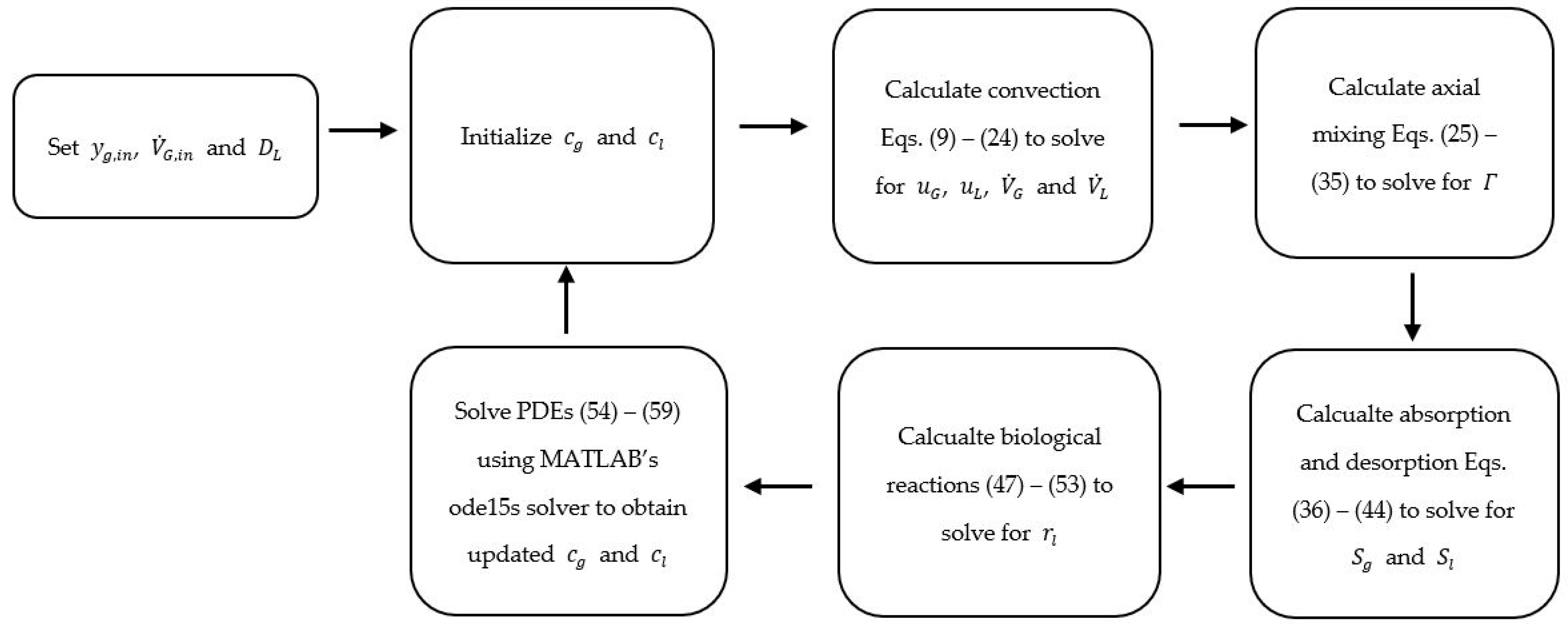
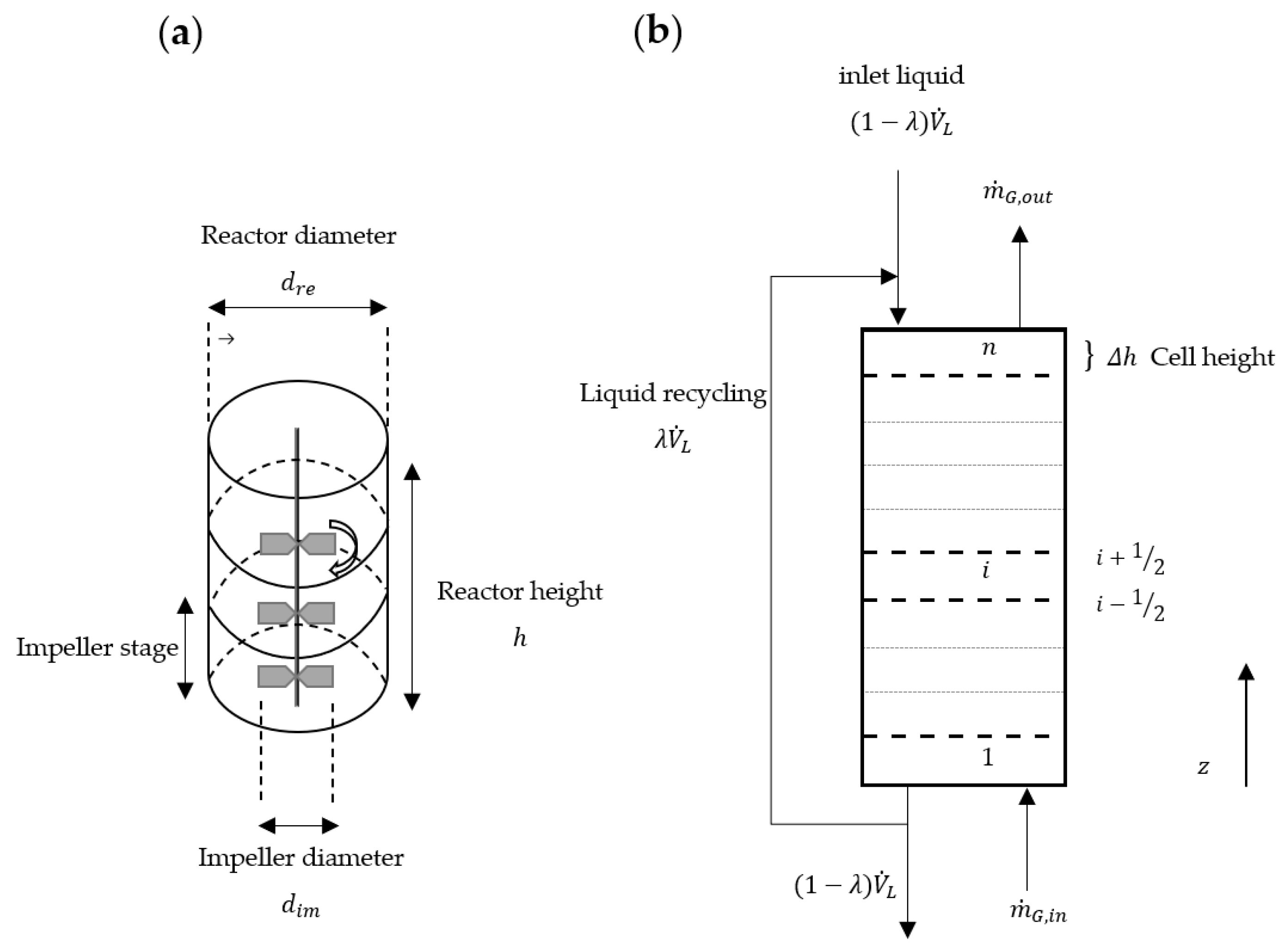
2. Materials and Methods

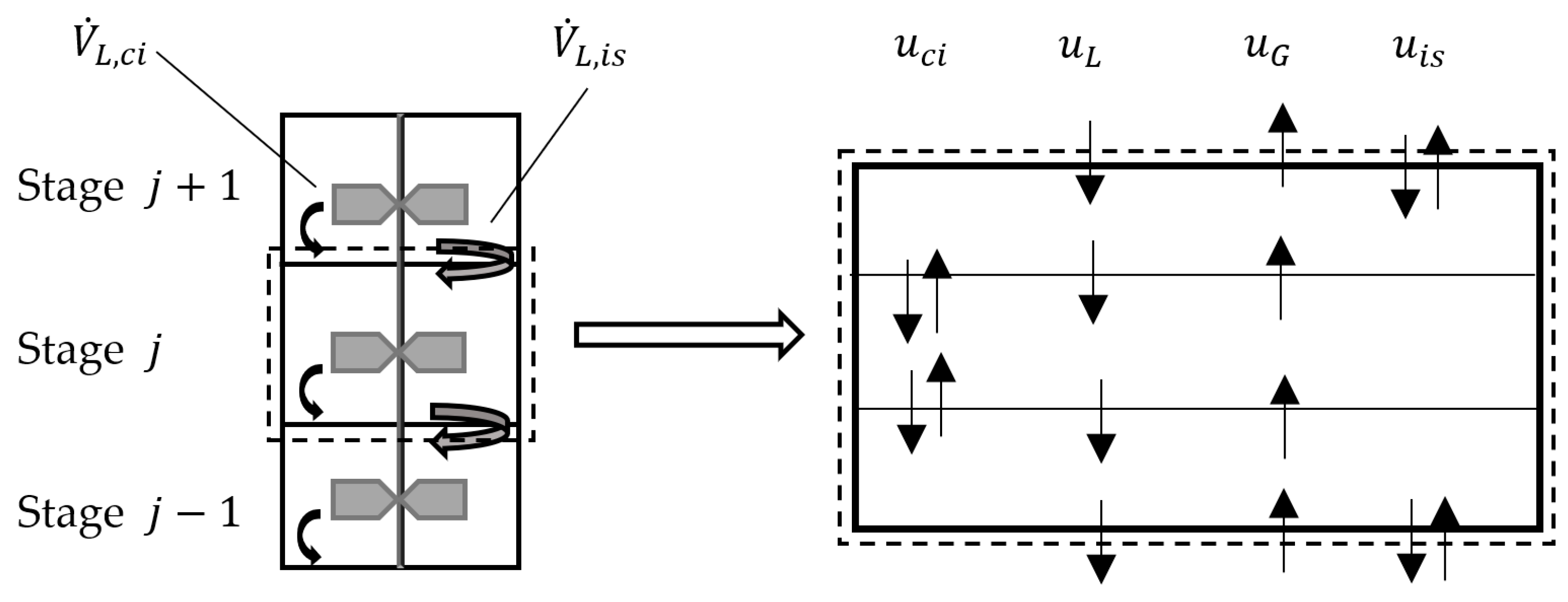
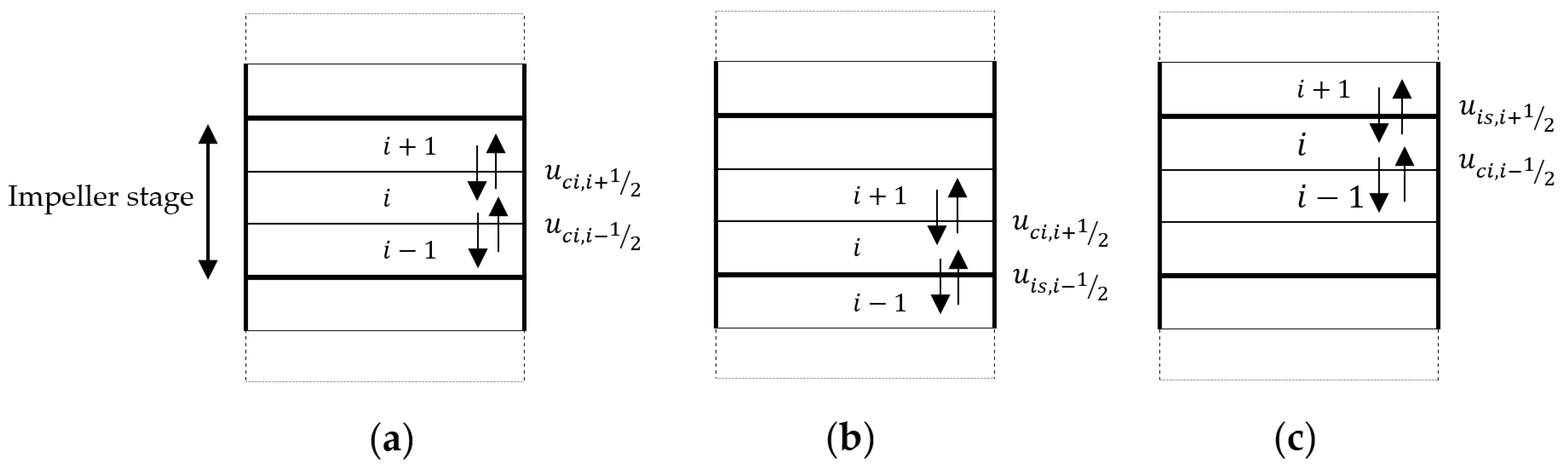
The model used in this study, based on the work of Inkeri et al. [11], is a one-dimensional representation of a biological methanation process in a continuous stirred tank reactor (CSTR). It incorporates semi-empirical correlations and partial differential mass conservation equations for the gas and liquid phases. The overall programming and initialization procedures, as well as assumptions for solving the component concentrations and other factors, have been modified in this study. Additionally, some equations and parameters have been revised to better align with the specific process under investigation. All the changes made in this study have been duly documented.

Equations (3) and (4) represent the mass balance for the gas and liquid phase concentrations, respectively. These equations account for convection, axial mixing (diffusion), absorption and desorption (gas–liquid mass transfer), and reaction rates (only in the liquid phase). It is worth noting that Equation (4) has been corrected in this study as it was found to be inaccurately written in the original work by Inkeri:

$$\frac{d{c}_g}{dt}=-\frac{d\left(u_G{c}_g\right)}{dz}+\frac{d}{dz}\left(\Gamma \frac{d{c}_g}{dz}\right)-S_g$$

(3)

$$\frac{d{c}_l}{dt}=\frac{d\left(u_L{c}_l\right)}{dz}+\frac{d}{dz}\left(\Gamma \frac{d{c}_l}{dz}\right)+S_l-r_l$$

(4)

where $c_g$ is the gas concentration, which is moles of gas per reactor volume ($\mathrm{mol}·{\mathrm{m}}^{-3}$); $c_l$ is the absorbed gas substance in moles per liquid volume ($\mathrm{mol}·{\mathrm{m}}^{-3}$); $u_G$ is the gas velocity ($\mathrm{m}·{\mathrm{s}}^{-1}$); $u_L$ is the liquid velocity ($\mathrm{m}·{\mathrm{s}}^{-1}$); $\Gamma$ is the axial mixing coefficient (${\mathrm{m}}^2·{\mathrm{s}}^{-1}$); $S_g$ is the source term for gas phase due to absorption/desorption ($\mathrm{mol}·{\mathrm{m}}^{-3}·{\mathrm{s}}^{-1}$); $S_l$ is the source term for liquid phase due to absorption/desorption ($\mathrm{mol}·{\mathrm{m}}^{-3}·{\mathrm{s}}^{-1}$); $r_l$ is the volumetric conversion rate for liquid phase (since biomass growth happens only in the liquid) ($\mathrm{mol}·{\mathrm{m}}^{-3}·{\mathrm{s}}^{-1}$).

Figure 1 [11] provides an overall schematic of the key phenomena in the reactor. In this study, radial gradients are neglected, and a plug flow model with superimposed axial mixing is used for both the liquid and gas phases. Plug flow refers to the ideal flow of fluid plugs in which all particles in a given cross-section, or element, have the same velocity and direction. It is assumed that there is little to no back-mixing of particles, and they all have the same residence time. Each plug of fluid is assumed to be uniform in composition, pressure, and temperature, and radial mixing is assumed to be infinitely fast [21]. The model’s calculation sequence is outlined in Figure 2, referencing the relevant equations.

As demonstrated in Figure 3 [11], the direction z is from bottom to top. The entire discretized space represents the portion of the reactor submerged in water with a constant height $h \left(\mathrm{m}\right)$, as both the liquid feed rate $D_L \left({\mathrm{s}}^{-1}\right)$ and gas inflow rate ${\dot{V}}_{G,in} \left({\mathrm{m}}^3·{\mathrm{s}}^{-1}\right)$ remain constant throughout the simulation. The gas phase components considered in this work are ${\mathrm{H}}_2$, ${\mathrm{CO}}_2$, and ${\mathrm{CH}}_4$, while in the liquid phase, they are ${\mathrm{H}}_2$, ${\mathrm{CO}}_2$, ${\mathrm{CH}}_4$, and biomass. Water is treated as bulk liquid and is not explicitly modeled. Each component is calculated separately, with G and L indices used for variables related to the gas or liquid phase, respectively. On the other hand, g and l indices are used for variables related to individual components.

2.1. Convection

A first-order upwind scheme for the convection Equations (5) and (6) is used to solve the major flows of liquid and gas. A minus sign in Equation (5) in Inkeri has been corrected.

$$\begin{gathered} \frac{d(u_G{c}_g)}{dz}\approx \frac{u_{G,i}{c}_{g,i}-u_{G,i-1}{c}_{g,i-1}}{\mathsf{\Delta }h} \\ \mathrm{for}i=2, 3, \dots , n \end{gathered}$$

(5)

$$\begin{gathered} \frac{d(u_L{c}_l)}{dz}\approx -\frac{u_{L,i}{c}_{l,i}-u_{L,i+1}{c}_{l,i+1}}{\mathsf{\Delta }h} \\ \mathrm{for}i=1, 2, 3, \dots , n-1 \end{gathered}$$

(6)

where $\mathsf{\Delta }h$ is the distance between two grid cells (m), and $i$ is the grid index.

Equations (5) and (6) were extended with boundary conditions (7) and (8), which were also corrected. Note that in Inkeri in Equation (7), the term $\Delta h$ was missing, and a minus sign was incorrectly assigned; also in Equation (8), the term $\left(1-{\varphi }_{\upsilon ,n}\right)\Delta h$ was incorrectly missing.

$$\frac{d\left(u_{G,1}{c}_{g,1}\right)}{dz}\approx \frac{u_{G,1}{c}_{g,1}}{\Delta h}-\frac{{\dot{m}}_{g,in}}{M_{g}A\Delta h}$$

(7)

$$\frac{d\left(u_{L,n}{c}_{l,n}\right)}{dz}\approx -\frac{u_{L,n}{c}_{l,n}}{\Delta h}+\lambda \frac{{\dot{V}}_L}{\left(1-{\varphi }_{\upsilon ,n}\right)A\Delta h}{c}_{l,1}$$

(8)

where $A$ is the cross-sectional area of the reactor (${\mathrm{m}}^2$); ${\varphi }_{\upsilon }$ is the gas hold-up with viscous effects ($-$); $\lambda$ is the liquid recycle constant, which is the fraction of liquid that is recycled to the inlet, which in the case of an overflow is assumed zero ($-$); $M_g$ is the molar mass of each gas component ($\mathrm{kg}·{\mathrm{mol}}^{-1}$); ${\dot{m}}_{g,in}$ is the inlet mass flux ($\mathrm{kg}·{\mathrm{s}}^{-1}$); ${\dot{V}}_L$ is the liquid volume flow rate, which is constant and needs not to be calculated at each time step (${\mathrm{m}}^3·{\mathrm{s}}^{-1}$).

The initialization process for the model involves several steps. First, the gas and liquid concentrations, $c_{g,0}$ and $c_{l,0}$, respectively, must be initialized, along with setting the inlet gas molar fractions, $y_{g,in}$. This inlet gas molar fraction, $y_{g,in}$, is later used to determine the inlet mass flux, ${\dot{m}}_{g,in}$. Additionally, based on the volume and amount of the incoming gaseous mixture, it is possible to estimate the initial gas concentrations of the model using $y_{g,in}$. However, unlike Inkeri et al. [11], who initialized $c_g$, $c_l$, $u_G$, and $u_L$ simultaneously, in this study, after initializing $c_g$ and $c_l$, other parameters are calculated until $u_G$ and $u_L$ are reached, as $u_G$ and $u_L$ are determined based on $c_g$ and $c_l$. It is important to note that, following Inkeri et al. [11], the concentration of biomass should typically be maintained below 15 g/L to ensure that the liquid’s hydrodynamic properties are similar to water, as commonly observed in practical applications. The first parameter after initialization to obtain is ${\varphi }_{\upsilon }$. To do so, two equations for calculating pressure will be used:

$$P_i=P_{re}+{\rho }_{L}g\Delta h\left(\frac{1-{\varphi }_{\upsilon ,i}}{2}+{\displaystyle \sum }_{j=i+1}^n(1-{\varphi }_{\upsilon ,j})\right)$$

(9)

$$P_i=\frac{RT{{\displaystyle \sum }}_g{c}_{g,i}}{{\varphi }_{\upsilon ,i}}$$

(10)

where $g=9.81\mathrm{m}·{\mathrm{s}}^{-2}$ is the gravitational constant; $R=8.314$ $\mathrm{J}·{\mathrm{mol}}^{-1}·{\mathrm{K}}^{-1}$ is the universal gas constant; $T=60°\mathrm{C}=333.15\mathrm{K}$ is the reactor temperature, which is considered constant during the simulations; ${\rho }_{\mathrm{L}}=1000\mathrm{kg}·{\mathrm{m}}^{-3}\mathrm{is}\mathrm{the}$constant liquid water density; $P_{re}=101325\mathrm{Pa}$ is the reactor overhead pressure that could be the atmospheric pressure or any other value; $P_i$is the pressure of each cell ($\mathrm{Pa}$).

The pressure in the reactor can be expressed as the sum of the overhead pressure and the hydrostatic pressure of water, which varies depending on the reactor height in each cell. This relationship is captured by Equation (9). On the other hand, Equation (10) represents the ideal gas law. When these two equations are combined, a quadratic Equation (11) is obtained:

$$\frac{{\rho }_{L}g\Delta h}{2}{\varphi }_{\upsilon ,i}{}^2-\left(P_{re}+{\rho }_{L}g\Delta h\left(n-i+\frac{1}{2}-{\displaystyle \sum }_{j=i+1}^n{\varphi }_{\upsilon ,j}\right)\right){\varphi }_{\upsilon ,i}+RT{\displaystyle \sum }_g{c}_{g,i}=0$$

(11)

which, after solving, would result in ${\varphi }_{\upsilon }$, which could be used to calculate the pressure either using Equation (9) or Equation (10). Other parameters are obtained afterwards:

$$y_{g,i,j}=\frac{c_{g,i,j}}{{{\displaystyle \sum }}_{j=1}^{n=3}{c}_{g,i,j}}$$

(12)

where $y_{g,i,j}$ is the molar fraction of gas component, $j$ in the corresponding cell $i$ ($-$), and $n=3$, because in each cell there are three gas components of ${\mathrm{CH}}_4$, ${\mathrm{CO}}_2$, and ${\mathrm{H}}_2$.

$$M_{G,i}={\displaystyle \sum }_{j=1}^{n=3}{y}_{g,i,j}{M}_{g,j}$$

(13)

where $M_{G,i}$ is the molar mass of the gas mixture in each cell, and $M_{g,j}$ is the molar mass of each gas component ($\mathrm{kg}·{\mathrm{mol}}^{-1}$). Furthermore, the biomass has a molar mass of 0.023306 $\mathrm{kg}·{\mathrm{mol}}^{-1}$.

$${\rho }_{G,i}=\frac{M_{G,i}{P}_i}{RT}$$

(14)

where ${\rho }_{G,i}$ is the ideal gas mixture density of the corresponding cell at the reactor temperature $T$ and pressure $P_i$ ($\mathrm{kg}·{\mathrm{m}}^{-3}$). According to Wilke’s mixing rule [22], the gas mixture viscosity at each cell is calculated with Equation (15):

$${\mu }_{G,i}={\displaystyle \sum }_{j=1}^{n=3}\frac{{\mu }_{g,j}}{1+\frac{1}{y_{g,i,j}}{{\displaystyle \sum }}_{\begin{array}{c}k=1\\ k\ne j\end{array}}^{k=n}{y}_{g,i,k}Ph{i}_{jk}}$$

(15)

where ${\mu }_g$ is the dynamic viscosity of each gas component at reactor temperature ($\mathrm{Pa}·\mathrm{s}$); values of dynamic viscosity can be seen in

Table 2. Gas components’ dynamic viscosities.

${\mathit{\mu }}_{\mathit{g}}$	$(\mathbf{P}\mathbf{a}\mathbf{·}\mathbf{s}$$)\times {10}^{-6}$
${\mathrm{CH}}_4$	11.993487
${\mathrm{CO}}_2$	16.330336
${\mathrm{H}}_2$	9.747077

[23]. Additionally, $Ph{i}_{jk}$ is defined as:

$$Ph{i}_{jk}=\frac{{\left[1+{\left(\raisebox{1ex}{${\mu }_{g,j}$}\!\left/ \!\raisebox{-1ex}{${\mu }_{g,k}$}\right.\right)}^{\frac{1}{2}}{\left(\raisebox{1ex}{$M_{g,k}$}\!\left/ \!\raisebox{-1ex}{$M_{g,j}$}\right.\right)}^{\frac{1}{4}}\right]}^2}{\raisebox{1ex}{$4$}\!\left/ \!\raisebox{-1ex}{$\sqrt{2}$}\right.{\left[1+\left(\raisebox{1ex}{$M_{g,j}$}\!\left/ \!\raisebox{-1ex}{$M_{g,k}$}\right.\right)\right]}^{\frac{1}{2}}}$$

(16)

According to Garcia-Ochoa et al. [24]:

$$\frac{{\varphi }_{\upsilon ,i}}{1-{\varphi }_{\upsilon ,i}}=\frac{{\varphi }_i}{1-{\varphi }_i}{\left(\frac{{\mu }_L}{{\mu }_{G,i}}\right)}^{-\raisebox{1ex}{$1$}\!\left/ \!\raisebox{-1ex}{$4$}\right.}$$

(17)

$$\frac{{\varphi }_i}{1-{\varphi }_i}=0.819\frac{U_{G,i}{}^{\raisebox{1ex}{$2$}\!\left/ \!\raisebox{-1ex}{$3$}\right.}{N}^{\raisebox{1ex}{$2$}\!\left/ \!\raisebox{-1ex}{$5$}\right.}{d}_{im}{}^{\raisebox{1ex}{$4$}\!\left/ \!\raisebox{-1ex}{$15$}\right.}}{g^{\raisebox{1ex}{$1$}\!\left/ \!\raisebox{-1ex}{$3$}\right.}}{\left(\frac{{\rho }_L}{\sigma }\right)}^{\raisebox{1ex}{$1$}\!\left/ \!\raisebox{-1ex}{$5$}\right.}\left(\frac{{\rho }_L}{{\rho }_L-{\rho }_{G,i}}\right){\left(\frac{{\rho }_L}{{\rho }_{G,i}}\right)}^{\raisebox{1ex}{$-1$}\!\left/ \!\raisebox{-1ex}{$15$}\right.}$$

(18)

where ${\varphi }_i$ is the gas hold-up without viscous effects at each cell ($-$); $U_{G,i}$ is the superficial velocity at each cell ($\mathrm{m}·{\mathrm{s}}^{-1}$); $N$ is the stirring speed ($\mathrm{rps}$); $d_{im}$ is the impeller diameter ($\mathrm{m}$); $\sigma =0.066 \mathrm{N}·{\mathrm{m}}^{-1}$ is the liquid surface tension at reactor temperature; ${\mu }_L=0.005 \mathrm{Pa}·\mathrm{s}$ is the water dynamic viscosity at reactor temperature. Solving Equation (17) gives us ${\varphi }_i$, and then using Equation (18), the superficial velocity $U_{G,i}$ is obtained. Following up, with Equation (19) the gas velocity $u_{G,i}$ and with Equation (20) the gas volume flow rate ${\dot{V}}_{G,i}$ at each cell are determined, along with other parameters afterwards:

$$u_{G,i}=\frac{U_{G,i}}{{\varphi }_{\mathsf{\upsilon },i}}$$

(19)

$${\dot{V}}_{G,i}=U_{G,i}A$$

(20)

where ${\dot{V}}_{G,i}$ is the gas volume flow rate at each cell (${\mathrm{m}}^3·{\mathrm{s}}^{-1}$).

$${\dot{V}}_L=D_{L}V$$

(21)

where $D_L$ is the liquid feed rate (${\mathrm{s}}^{-1}$), and $V$ is the active reactor volume (${\mathrm{m}}^3)$.

$$u_{L,i}=\frac{{\dot{V}}_L}{\left(1-{\varphi }_{\upsilon ,i}\right)A}$$

(22)

$$w_{g,in}=\frac{y_{g,in}{M}_g}{{{\displaystyle \sum }}_g{y}_{g,in}{M}_g}$$

(23)

where $w_{g,in}$ is the mass fraction of gas components at the inlet ($-)$.

$${\dot{m}}_{g,in}=w_{g,in}{\rho }_{G,1}{\dot{V}}_{G,in}$$

(24)

where ${\rho }_{G,1}$ is the density of the gas mixture at the inlet (first cell) ($\mathrm{kg}·{\mathrm{m}}^{-3}$), and ${\dot{V}}_{G,in}$ is the gas inflow rate (${\mathrm{m}}^3·{\mathrm{s}}^{-1}$).

2.2. Axial Mixing

Diffusion of the substrates inside the reactor happens because of the axial mixing flows due to the impeller’s rotation. A perfect mixing is assumed in a CSTR [25]. The axial mixing coefficient $\Gamma$ is defined with Equation (25), in which the axial mixing velocity is either $u_{ci}$ or $u_{is}$, depending on the position of the corresponding cell relative to the impeller stage. These velocities are defined on the interface of the cells; therefore, a mean value approach was used to determine their appropriate values after calculating them for each cell.

$$\Gamma =\{\begin{array}{c}{u}_{ci}\Delta h interiorface\\ u_{is}\Delta h inter-stage face\end{array}$$

(25)

where $\Gamma$ is the axial mixing coefficient (${\mathrm{m}}^2·{\mathrm{s}}^{-1}$); $u_{ci}$ is the circulation velocity describing the internal mixing under the stage influence of an impeller ($\mathrm{m}·{\mathrm{s}}^{-1}$); $u_{is}$ is the mixing velocity between two stages, since each impeller creates its own individual circulation flow pattern ($\mathrm{m}·{\mathrm{s}}^{-1}$). $u_{ci}$ and $u_{is}$ will be defined later in Equations (34) and (35).

As it is shown in Figure 4 [11], a unique circulation flow ${\dot{V}}_{L,ci}$ is produced by each impeller within its own impeller volume (stage). The inter-stage flow ${\dot{V}}_{L,is}$ is used to represent the liquid mixing between two stages. The mixing flows are used to compute the velocities $u_{ci}$ and $u_{is}$. The gas and liquid have the corresponding countercurrent main flow velocities of $u_G$ and $u_L$. Using the usual central difference discretization for second derivatives, axial mixing generated by stirring is defined by Equations (26) and (27) for gas and liquid phases, respectively. Mixing velocities are considered the same for both liquid and gas phases.

$$\frac{d}{dz}\left(\Gamma \frac{d{c}_g}{dz}\right)\approx \frac{{\Gamma }_{i-1/2}{c}_{g,i-1}-\left({\Gamma }_{i-1/2}+{\Gamma }_{i+1/2}\right)c_{g,i}+{\Gamma }_{i+1/2}{c}_{g,i+1}}{\Delta h^2}$$

(26)

$$\frac{d}{dz}\left(\Gamma \frac{d{c}_l}{dz}\right)\approx \frac{{\Gamma }_{i-1/2}{c}_{l,i-1}-\left({\Gamma }_{i-1/2}+{\Gamma }_{i+1/2}\right)c_{l,i}+{\Gamma }_{i+1/2}{c}_{l,i+1}}{\Delta h^2}$$

(27)

Figure 5 [11] illustrates how the mixing velocities on the interfaces in a stage are considered, whether interior or inter-stage faces. Vasconcelos et al. [26] argues that, under ungassed conditions, impellers create a rotating flow that creates a circulation backflow ${\dot{V}}_{L,ci0}$ between interior cells and an inter-stage mixing flow ${\dot{V}}_{L,is0}$ between two stirrers, which are described in Equations (28) and (29):

$${\dot{V}}_{L,ci0}=N_{ci0}N{d}_{im}{}^3$$

(28)

$${\dot{V}}_{L,is0}=N_{is0}N{d}_{im}{}^3$$

(29)

where ${\dot{V}}_{L,ci0}$ and ${\dot{V}}_{L,is0}$ are ungassed circulation and inter-stage liquid flow rates (${\mathrm{m}}^3·{\mathrm{s}}^{-1}$), and $N_{ci0}$ and $N_{is0}$ are circulation and inter-stage numbers ($-$), respectively. $N_{ci0}$ and $N_{is0}$ are constant if the flow is turbulent and dependent only on the impeller–reactor diameter ratio $\raisebox{1ex}{$d_{im}$}\!\left/ \!\raisebox{-1ex}{$d_{re}$}\right.$, which is true in this case and applicable. They are defined by the following equations:

$$N_{ci0}=b_1{\left(\frac{d_{re}}{d_{im}}\right)}^{1.8}$$

(30)

$$N_{is0}=b_2\left(\frac{d_{re}}{d_{im}}\right)$$

(31)

where $d_{re}$ is the reactor diameter ($m$), and $b_1=0.21$ and $b_2=0.236$ are the axial mixing constants ($-$). Now, the axial mixing flows under gassed conditions, ${\dot{V}}_{L,ci}$ and ${\dot{V}}_{L,is}$ (since gas sparges from underneath the reactor), should be calculated and then the axial mixing velocities, $u_{ci}$ and $u_{is}.$

$${\dot{V}}_{L,ci,i}=\frac{P_{t,i}}{P_{t0}}{\dot{V}}_{L,ci0}$$

(32)

$${\dot{V}}_{L,is,i}=\frac{P_{t,i}}{P_{t0}}{\dot{V}}_{L,si0}$$

(33)

where $P_{t,i}$ is the gassed stirring power at each cell ($\mathrm{W}$), which will be later defined in Equation (41); $P_{t0}$ is the ungassed stirring power ($\mathrm{W}$); ${\dot{V}}_{L,ci,i}$ and ${\dot{V}}_{L,is,i}$ are the gassed circulation and inter-stage liquid flow rates (${\mathrm{m}}^3·{\mathrm{s}}^{-1}$).

$$u_{ci,i}=\frac{{\dot{V}}_{L,ci,i}}{\left(1-{\varphi }_{v,i}\right)A}$$

(34)

$$u_{is,i}=\frac{{\dot{V}}_{L,is,i}}{\left(1-{\varphi }_{\upsilon ,i}\right)A}$$

(35)

After calculating $u_{ci}$ and $u_{is}$, Equation (25) is used to obtain the axial mixing coefficient values.

2.3. Absorption and Desorption

Gases are absorbed with the aid of stirring impellers into the bulk liquid and then to the archaea cells. Absorbed gases in the liquid are transported to the cellular surfaces of the biomass by convection and diffusion. Afterward, ${\mathrm{CH}}_4$ is produced and desorbed from the liquid to the gas. The driving factor for the transfer process is the difference between the saturation and the actual substrate concentration in the liquid ($c_l{}^{*}-c_l$). By absorption, transfer rates for gaseous $S_g$ have positive values and, in the case of desorption, negative. For the liquid phase, $S_g$ multiplies with the liquid hold-up since it depends on the reactor volume and results in $S_l$.

$$S_{g,i}=k_{L,g,i}{a}_i\left(c_{l,i}{}^{*}-c_{l,i}\right)$$

(36)

$$S_{l,i}=S_{g,i}\left(1-{\varphi }_{\upsilon ,i}\right)$$

(37)

where $c_{l,i}{}^{*}$ is the saturation solubility in the liquid in cell $i$ ($\mathrm{mol}·{\mathrm{m}}^{-3}$); $k_{L,g,i}$ is the mass transfer coefficient in cell $i$ ($\mathrm{m}·{\mathrm{s}}^{-1}$); $a_i$ is the interfacial area in cell $i$ (${\mathrm{m}}^{-1}$). Henry’s law, which takes temperature and pressure into account, is used to determine the saturation solubility $c_{l,i}{}^{*}$. The concentration of gas particles in the solution phase $c_{l,i}{}^{*}$ that are in equilibrium with the partial pressure of the gas in the gaseous phase $y_{g,i}{P}_i$, is related by Henry’s law constant $H_g$ [27], which is demonstrated in Equation (38).

$$c_{l,i}{}^{*}=H_g{y}_{g,i}{P}_i$$

(38)

where $y_{g,i}$ is the molar fraction of each gas component in the corresponding cell $i$ ($-$); $P_i$is the cell pressure in cell $i$ ($\mathrm{Pa}$) calculated by Equation (10); $H_g$ is the Henry’s solubility coefficient of each gas ($\mathrm{mol}·{\mathrm{m}}^{-3}·{\mathrm{Pa}}^{-1}$) calculated by Sander et al. [28]. Values in this case are shown in

Table 3. Henry’s solubility coefficients for gas components.

${\mathit{H}}_{\mathit{g}}$	$(\mathbf{mol}\mathbf{·}{\mathbf{m}}^{-3}\mathbf{·}\mathbf{P}{\mathbf{a}}^{-1}$$)\times {10}^{-5}$
${\mathrm{CH}}_4$	0.66
${\mathrm{CO}}_2$	13.25
${\mathrm{H}}_2$	0.60

[28].

The volumetric gas–liquid mass transfer coefficient $k_{L,g}a$ is predicted by the work of Garcia-Ochoa et al. [24]. This value is dependent on the reactor dimensions, stirring system properties, and operational conditions and can be used for designing reactor systems where no measured data are available. It is separated into two parameters, the mass transfer coefficient $k_{L,g}$ and the interfacial area $a$, and should be calculated for each gas separately, which are defined by the following equations:

$$k_{L,g,i}=\frac{2}{\sqrt{\pi }}\sqrt{D_g}{\left(\frac{{\epsilon }_i{\rho }_L}{{\mu }_L}\right)}^{\raisebox{1ex}{$1$}\!\left/ \!\raisebox{-1ex}{$4$}\right.}$$

(39)

where $D_g$ is the gas diffusivity in liquid (${\mathrm{m}}^2·{\mathrm{s}}^{-1}$), calculated by extrapolation from [29], and ${\epsilon }_i$ is the dissipated energy resulted from stirring power delivered by the impellers to the liquid through turbulent dissipation at each cell ($\mathrm{W}·{\mathrm{kg}}^{-1}$). The values of $D_g$ are presented in

Table 4. Gas diffusion coefficients in water at 60 °C.

${\mathit{D}}_{\mathit{g}}$	$({\mathbf{m}}^2\mathbf{·}{\mathbf{s}}^{-1}$$)\times {10}^{-9}$
${\mathrm{CH}}_4$	4.4597
CO2	4.8682
${\mathrm{H}}_2$	11.064

[29].

$${\epsilon }_i=\frac{P_{t,i}}{{\rho }_L\pi \frac{d_{re}{}^2}{4}\frac{h}{n_{im}}}$$

(40)

where $h$ is the reactor height ($\mathrm{m}$), and $n_{im}$ is the number of equally spaced impellers ($-$).

$P_t$ is the power needed in the gassed situation for stirring the substrates. If we increase the total inlet gas flow ${\dot{V}}_G$—which is the sum of the inflow rates of the three inlet gases, methane, carbon dioxide, and hydrogen—viscous resistance in the reactor decreases and, subsequently, the stirring power need to do so. Therefore, for example, for a constant stirring speed, lesser power is required with a higher gas inflow rate. According to Michel et al. [30]:

$$P_{t,i}=0.783{\left(\frac{P_{t0}{}^{2}N{d}_{im}{}^3}{{\dot{V}}_{G,i}{}^{0.56}}\right)}^{0.459}$$

(41)

To obtain the gassed stirring power, we need to calculate the ungassed stirring power $P_{t0}$, which depends on the power number $N_P$ ($-$), liquid density ${\rho }_L$ ($\mathrm{kg}·{\mathrm{m}}^{-3}$), stirring speed $N$ ($\mathrm{rps}$), and impeller diameter $d_{im}$ ($\mathrm{m}$). The power number is based on the details of the impeller geometry, which is provided by the manufacturers. Here, a traditional Rushton impeller with a power number of 7.0 is presented [31].

$$P_{t0}=N_P{\rho }_L{N}^3{d}_{im}{}^5$$

(42)

The second part of $k_{L,g}a$, the interfacial area $a$, is calculated with Equation (43). It consists of the average bubble size $d_b$ ($\mathrm{m}$) and the gas hold-up ${\varphi }_{\upsilon }$ ($-$). Both are linked with the fluid’s physical properties, flow characteristics, and reactor dimension. In addition, the average bubble size is calculated using Equation (44) as proposed by Bhavaraju et al. [32]. The assumption is that merging and breakup of bubbles are fast, so the bubble size is set to an average stable value.

$$a_i=\frac{6{\varphi }_{\upsilon ,i}}{d_{b,i}}$$

(43)

$$d_{b,i}=0.7\frac{{\sigma }^{0.6}}{{\left(\frac{P_{t,i}}{\raisebox{1ex}{$V$}\!\left/ \!\raisebox{-1ex}{$n_{im}$}\right.}\right)}^{0.4}{\rho }_L{}^{0.2}}{\left(\frac{{\mu }_L}{{\mu }_{G,i}}\right)}^{0.1}$$

(44)

2.4. Biological Reaction Kinetics

In this section, we discuss the reaction source term $r_l$ in Equation (4), which demonstrates the production or consumption of a component in the liquid phase. The reactants in this model are hydrogen, carbon dioxide, and ammonia, and the products are methane, biomass, and water. We assume that reaction rates do not depend on ammonia concentration. Additionally, ammonia is not considered a limiting factor in the reaction, and it is assumed that there is always enough of it in the reactor. Water production is also small compared to the water content in the reactor. Therefore, we do not account for the concentration and reaction rates of ammonia and water in our model.

The methanation of carbon dioxide and hydrogen, which results in methane, is due to the growth of the archaeon Methanobacterium thermoautotrophicum [11]. The necessary energy for this matter is generated by the oxidation of ${\mathrm{H}}_2$ and the associated reduction of ${\mathrm{CO}}_2$ to ${\mathrm{CH}}_4$ [12]. Equation (45) represents the elemental composition of the biomass, reactants, and products of the methanogenesis reaction [12]. Equation (45), however, is insufficient to adequately represent the microbial system. A non-negligible extra amount of ${\mathrm{H}}_2$ is consumed to produce ${\mathrm{CH}}_4$, which provides the energy required for M. thermoautotrophicum’s maintenance processes [33]. This maintenance reaction is described in Equation (46). Equations (45) and (46) describe the coefficients of ${\mathrm{CO}}_2$and ${\mathrm{H}}_2$ and are used to calculate the ${\mathrm{CH}}_4$ yield. All the subscripts are presented in

Table 5. Subscript indices for components.

Components	Subscripts
${\mathrm{H}}_2$	D
${\mathrm{CO}}_2$	C
${\mathrm{CH}}_4$	P
${\mathrm{NH}}_3$	N
${\mathrm{H}}_2\mathrm{O}$	W
Biomass	X

[11].

$${\mathrm{H}}_2+Y_{C/D}{\mathrm{CO}}_2+Y_{N/D}{\mathrm{NH}}_3\to Y_{X/D}{\mathrm{CH}}_{1.68}{\mathrm{O}}_{0.39}{\mathrm{N}}_{0.24}+Y_{P/D}{\mathrm{CH}}_4+Y_{W/D}{\mathrm{H}}_2\mathrm{O}$$

(45)

$$4{\mathrm{H}}_2+{\mathrm{CO}}_2\to {\mathrm{CH}}_4+2{\mathrm{H}}_2\mathrm{O}$$

(46)

The stoichiometric consumption and yield of substrates are also depicted in

Table 6. Molar yield coefficients [mol/mol] and parameters related to biomass growth (archaea).

${\mathit{Y}}_{\mathit{X}/\mathit{D}}$	Subscripts	$\mathbf{m}\mathbf{o}{\mathbf{l}}_{\mathbf{X}}/\mathbf{m}\mathbf{o}{\mathbf{l}}_{\mathbf{D}}$
$Y_{N/D}$	0.00456	${\mathrm{mol}}_{\mathrm{N}}/{\mathrm{mol}}_{\mathrm{D}}$
$Y_{C/D}$	0.259	${\mathrm{mol}}_{\mathrm{C}}/{\mathrm{mol}}_{\mathrm{D}}$
$Y_{P/D}$	0.24	${\mathrm{mol}}_{\mathrm{P}}/{\mathrm{mol}}_{\mathrm{D}}$
$Y_{W/D}$	0.511	${\mathrm{mol}}_{\mathrm{W}}/{\mathrm{mol}}_{\mathrm{D}}$
$k_D$	5.6	$\left[\mathrm{mol}·{\mathrm{m}}^{-3}\right]\ast {10}^{-3}$
${\mu }^{max}$	0.361 (± 0.011)	$\left[{\mathrm{s}}^{-1}\right]/3600$
$m_X$	1.67 (± 0.46)	$\left[\mathrm{mol}·{\mathrm{mol}}^{-1}·{\mathrm{s}}^{-1}\right]/3600$

[12]. Based on Schill et al. [12], values for yield were computed according to the measured biomass yield $Y_{X/D}=0.019$ ${\mathrm{mol}}_{\mathrm{x}}/{\mathrm{mol}}_{\mathrm{D}}$ and the elemental composition of the biomass. To have a more accurate model, these constants should change to match the specific environment of the archaea used. In the meantime, the following parameters must be calculated: maximum consumption of ${\mathrm{H}}_2$, $q^{max}$ with Equation (48), ${\mathrm{H}}_2$ consumption rate $r_D$ with Equation (47), and following up the production and consumption rates of other substances using Equations (49)–(51). It is mentionable that the original signs of Equations (49)–(51) were mistakenly assigned, which were corrected here. Equation (47) is based on the Monod equation. The most popular rate expression for describing the growth of microorganisms in general, and hydrogen-producing bacteria in particular, is the empirical Monod equation. This is equivalent to a hyperbolic function in which the specific growth rate $r_D$ is related to the concentration of the substrates $c_D$ and $c_X$ [34].

$$r_{D,i}=q^{max}\frac{c_{D,i}}{c_{D,i}+k_D}{c}_{X,i}{I}_{C,i}$$

(47)

where $r_{D,i}$ is the ${\mathrm{H}}_2$volumetric conversion rate in cell $i$ ($\mathrm{mol}·{\mathrm{m}}^{-3}·{\mathrm{s}}^{-1}$); $q^{max}$ is the maximum specific ${\mathrm{H}}_2$ conversion rate ($\mathrm{mol}·{\mathrm{mol}}^{-1}·{\mathrm{s}}^{-1}$); $c_{D,i}=c_{l,3,i}$ is the ${\mathrm{H}}_2$ concentration in liquid in cell $i$ ($\mathrm{mol}·{\mathrm{m}}^{-3}$); $k_D$ is the saturation constant for ${\mathrm{H}}_2$ ($\mathrm{mol}·{\mathrm{m}}^{-3}$); $c_{X,i}=c_{l,4,i}$ is the biomass concentration in liquid in cell $i$ ($\mathrm{mol}·{\mathrm{m}}^{-3}$); $I_{C,i}$ is the inhibition factor due to the lack of ${\mathrm{CO}}_2$ in cell $i$ ($-$). $k_D$ is defined in Table 6, and $I_{C,i}$ is defined in Equation (53).

$$q^{max}=\frac{{\mu }^{max}+Y_{X/D}{m}_X}{Y_{X/D}}$$

(48)

where ${\mu }^{max}$ is the maximum growth rate of biomass (${\mathrm{s}}^{-1}$) and is defined in Table 6; $Y_{X/D}$ is the biomass molar yield (${\mathrm{mol}}_{\mathrm{x}}/{\mathrm{mol}}_{\mathrm{D}}$), and $m_X$ is the maintenance constant ($\mathrm{mol}·{\mathrm{mol}}^{-1}·{\mathrm{s}}^{-1}$) and is also defined in Table 6.

$$r_{X,i}=-Y_{X/D}\left(r_{D,i}-m_X{c}_{X,i}{I}_{C,i}{I}_{D,i}\right)$$

(49)

where $r_{X,i}$ is the biomass volumetric conversion rate in cell $i$ ($\mathrm{mol}·{\mathrm{m}}^{-3}·{\mathrm{s}}^{-1}$), and $I_{D,i}$ is the inhibition factor due to the lack of ${\mathrm{H}}_2$ in cell $i$ ($-$).

$$r_{C,i}=Y_{C/D}{r}_{D,i}+\left(\frac{1}{4}-Y_{C/D}\right)m_X{c}_{X,i}{I}_{C,i}{I}_{D,i}$$

(50)

where $r_{C,i}$ is the ${\mathrm{CO}}_2$ volumetric conversion rate in cell $i$ ($\mathrm{mol}·{\mathrm{m}}^{-3}·{\mathrm{s}}^{-1}$), and $Y_{C/D}$ is the ${\mathrm{CO}}_2$ molar yield (${\mathrm{mol}}_{\mathrm{C}}/{\mathrm{mol}}_{\mathrm{D}}$).

$$r_{P,i}=-\left(Y_{P/D}{r}_{D,i}+\left(\frac{1}{4}-Y_{P/D}\right)m_X{c}_{X,i}{I}_{C,i}{I}_{D,i}\right)$$

(51)

where $r_{P,i}$ is the ${\mathrm{CH}}_4$ volumetric conversion rate in cell $i$ ($\mathrm{mol}·{\mathrm{m}}^{-3}·{\mathrm{s}}^{-1}$), and $Y_{P/D}$ is the ${\mathrm{CH}}_4$ molar yield (${\mathrm{mol}}_{\mathrm{P}}/{\mathrm{mol}}_{\mathrm{D}}$). Ammonia and water reaction rates are not required to be calculated, since they do not have any effect on our modeling. As was discussed before, biomass growth and methane production decrease if the stoichiometric amount of reactant substances (hydrogen and carbon dioxide) are not provided as they should, according to the equations. Eventually, reactions will cease if the substance concentrations go near zero. The maintenance reaction for the biomass requires dissolved ${\mathrm{CO}}_2$and ${\mathrm{H}}_2$. The inhibition factors are defined by Equations (52) and (53).

$$I_{D,i}=\frac{1}{1+\frac{{10}^{-3}}{c_{D,i}}}$$

(52)

$$I_{C,i}=\frac{1}{1+\frac{{10}^{-3}}{c_{C,i}}}$$

(53)

where $c_{C,i}=c_{l,2,i}$ is the ${\mathrm{CO}}_2$ concentration in liquid in cell $i$ ($\mathrm{mol}·{\mathrm{m}}^{-3}$).

After discretization and applying the boundary conditions, Equations (3) and (4) become the following initial value ODEs for the mentioned indexes $i$, of which the goal would be to obtain concentrations $c_g$ and $c_l$; they are solved in MATLAB using the ode15s solver:

$$\frac{d{c}_{g,i}}{dt}=-\frac{u_{G,1}{c}_{g,1}}{\Delta h}+\frac{{\dot{m}}_{g,in}}{M_{g}A\Delta h}+\frac{-\left({\Gamma }_{i-1/2}+{\Gamma }_{i+1/2}\right)c_{g,i}+{\Gamma }_{i+1/2}{c}_{g,i+1}}{\Delta h^2}-S_{g,i}$$

(54)

$$\begin{gathered} \frac{d{c}_{l,i}}{dt}=-\frac{u_{L,i}{c}_{l,i}-u_{L,i+1}{c}_{l,i+1}}{\Delta h}+\frac{-\left({\Gamma }_{i-1/2}+{\Gamma }_{i+1/2}\right)c_{l,i}+{\Gamma }_{i+1/2}{c}_{l,i+1}}{\Delta h^2}+S_{l,i}-r_{l,i} \\ \mathrm{for}i=1 \end{gathered}$$

(55)

$$\frac{d{c}_{g,i}}{dt}=-\frac{u_{G,i}{c}_{g,i}-u_{G,i-1}{c}_{g,i-1}}{\Delta h}+\frac{{\Gamma }_{i-1/2}{c}_{g,i-1}-\left({\Gamma }_{i-1/2}+{\Gamma }_{i+1/2}\right)c_{g,i}+{\Gamma }_{i+1/2}{c}_{g,i+1}}{\Delta h^2}-S_{g,i}$$

(56)

$$\begin{gathered} \frac{d{c}_{l,i}}{dt}=-\frac{u_{L,i}{c}_{l,i}-u_{L,i+1}{c}_{l,i+1}}{\Delta h}+\frac{{\Gamma }_{i-1/2}{c}_{l,i-1}-\left({\Gamma }_{i-1/2}+{\Gamma }_{i+1/2}\right)c_{l,i}+{\Gamma }_{i+1/2}{c}_{l,i+1}}{\Delta h^2}+S_{l,i}-r_{l,i} \\ \mathrm{for}i=2,3,\dots ,n-1 \end{gathered}$$

(57)

$$\frac{d{c}_{g,i}}{dt}=-\frac{u_{G,i}{c}_{g,i}-u_{G,i-1}{c}_{g,i-1}}{\Delta h}+\frac{{\Gamma }_{i-1/2}{c}_{g,i-1}-\left({\Gamma }_{i-1/2}+{\Gamma }_{i+1/2}\right)c_{g,i}}{\Delta h^2}-S_{g,i}$$

(58)

$$\begin{gathered} \frac{d{c}_{l,i}}{dt}=-\frac{u_{L,n}{c}_{l,n}}{\Delta h}+\lambda \frac{{\dot{V}}_L}{\left(1-{\varphi }_{\upsilon ,n}\right)A\Delta h}{c}_{l,1}+\frac{{\Gamma }_{i-1/2}{c}_{l,i-1}-\left({\Gamma }_{i-1/2}+{\Gamma }_{i+1/2}\right)c_{l,i}}{\Delta h^2}+S_{l,i}-r_{l,i} \\ \mathrm{for}i=n \end{gathered}$$

(59)

Equations (54)–(59) are considered stiff equations. A stiff ordinary differential equation problem occurs when the solution being sought is changing slowly, but surrounding solutions are changing quickly. To produce results, the numerical approach must make modest increments [35]. Explicit approaches, such as the explicit Euler method, are unsuccessful to solve the equations, even when the time step is set to be extremely small. Implicit methods are much better suited to solve stiff problems. While taking much larger time steps, approaches designed to effectively address stiff problems do more work per step. They solve a set of concurrent linear equations at each stage using MATLAB matrix operations to forecast how the solution will develop [35]. As suggested by Inkeri, the implicit variable order approach of MATLAB’s ode15s solver was used to solve these sets of equations [11,36].

3. Results

Three models based on experimental data, Schill et al. [12], Seifert et al. [8], and Martin et al. [14], were simulated and compared with each other to obtain an initial impression of the functionality of the model with different reactor geometry parameters such as: active reactor volume $V$, reactor height–diameter ratio $h:d_{re}$, impeller diameter $d_{im}$, stirring speed $N$, and number of impellers $n_{im}$. These parameters are published values, and Inkeri assumed the missing information denoted by an asterisk in

Table 7. Description of the modeled reactors. * denotes assumed values.

Model	$\mathit{V} \left(\mathbf{L}\right)$	$\mathit{h}:{\mathit{d}}_{\mathit{r}\mathit{e}} (-)$	${\mathit{d}}_{\mathit{i}\mathit{m}} \left(\mathit{m}\right)$	$\mathit{N} \left(\mathbf{r}\mathbf{p}\mathbf{m}\right)$	${\mathit{n}}_{\mathit{i}\mathit{m}} (-)$	$\mathit{T} \left(°\mathbf{C}\right)$
Schill	1.5	2:1 *	0.07	1000	1	60
Seifert	4.25	2:1 *	0.06	1500	3	60
Martin	3.25	2:1 *	0.06	700	4	60

[11].

The operating temperature of all three cases is 60 °C, which means the physical properties, such as dynamic viscosities ${\mu }_g$ and ${\mu }_L$, liquid density ${\rho }_L$, diffusion coefficients $D_g$, and Henry’s solubility coefficients $H_g,$ are equal in all three. A gas inflow rate of ${\dot{V}}_{G,in}=0.5 \mathrm{vvm}$ (gas volume flow per liquid volume in a minute) and liquid feed rate of $D_L=0.2 1/\mathrm{h}$ were set for all three simulations. Overhead pressure of the reactor was set at atmospheric pressure of $P_{re}=101325 \mathrm{Pa}$, with a liquid recycle constant of $\lambda =0.5$. For a more precise calculation, ten cells were assigned to each impeller stage for the simulations. In addition, the simulation time of every case was chosen differently to observe the concentration change in the substrates for different durations.

It is assumed that pure ${\mathrm{CO}}_2$ is supplied by the biogas plant and ${\mathrm{H}}_2$ is added in a stoichiometric amount. Additionally, according to the maintenance reaction in Equation (46), the stochiometric ratio of ${\mathrm{H}}_2:{\mathrm{CO}}_2$is 4:1. Therefore, the inlet molar fraction of the gas mixture would be $y_{g,in}=\left[\begin{array}{c}0: {\mathrm{CH}}_4\\ 0.2: {\mathrm{CO}}_2\\ 0.8: {\mathrm{H}}_2\end{array}\right]$. $c_{g,0}$ is the initial condition, and $y_{g,in}$ is the boundary condition. Therefore, $c_{g,0}$ could be either calculated based on $y_{g,in}$ or be defined separately. For $c_{l,0}$, since initially there is not any gas in the liquid medium, and on the other hand, there has to exist a biomass concentration for the biological reactions to initiate, the initial liquid concentration is set to $c_{l,0}=\left[\begin{array}{c}0: {\mathrm{CH}}_4\\ 0: {\mathrm{CO}}_2\\ \begin{array}{c}0: {\mathrm{H}}_2\\ 40:\mathrm{Biomass}\end{array}\end{array}\right]\mathrm{mol}·{\mathrm{m}}^{-3}$.

As demonstrated in Figure 6, all three cases reach stability in ${\mathrm{CH}}_4\left(\mathrm{g}\right)$ concentration after about 50 s. In all of the cases, raising the reactor height, methane is produced, and $C_p\left(g\right)$ increases. Steady-state happens in $C_c\left(g\right)$ roughly after 700 s in Schill, 20 s in Seifert, and 300 s in Martin. All the simulations indicate lower ${\mathrm{CO}}_2\left(\mathrm{g}\right)$ concentration at the top of the reactor than at the bottom, which indicates the consumption of ${\mathrm{CO}}_2$ to produce methane and for biomass to grow. Schill predicts stability in ${\mathrm{H}}_2\left(\mathrm{g}\right)$ concentration after approximately 400 s, Seifert after 60 s, and Martin after 150 s. Here also, by increasing the reactor height, $C_D\left(g\right)$ decreases. As it can be seen in all the experiments, biomass concentration $C_X\left(l\right)$ increases over time and does not seem much to be affected by reactor height. In addition, the longer the simulation time, the more uniform the concentrations appear alongside the reactor height. In Schill’s model, they are completely uniform.

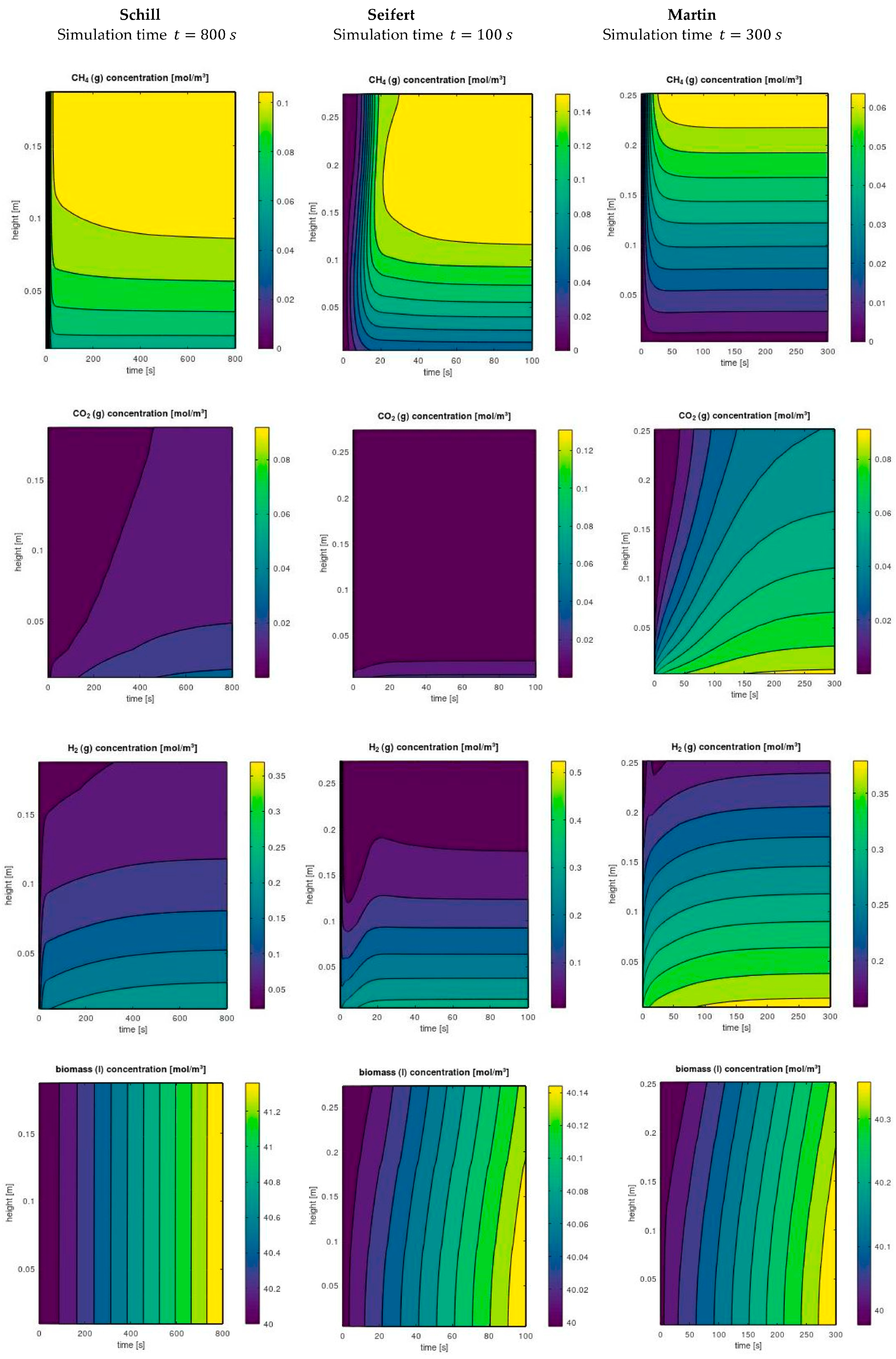
3.1. Model Validation

To validate the capability of the model, a comparison between model predictions and measured values from the literature was performed. These experimental data were published in Schill et al. [12], Seifert et al. [8], and Martin et al. [14] with their reactor configurations presented in Table 7. The experiments did not indicate any liquid recycling, so the liquid recycle constant λ was set to 0 for all cases. Additionally, since no continuous feeding was observed in the Martin experiment, the liquid feed rate $D_L$ was also set to 0. The Seifert experiment was conducted at 65 °C, while Schill and Martin were performed at 60 °C. As a result, two sets of physical properties were defined to account for these different temperatures. Additionally, in these experiments, the total reactor volume $V_{tot}$ was taken into account in addition to the active reactor volume $V$. Schill’s, Seifert’s, and Martin’s reactors have total volumes of 2.0 L, 10.0 L, and 7.5 L, respectively [11]. The methane production rates $r_P\left(l\right)$ in this section are converted to standard temperature and pressure (STP) conditions, with a temperature of 0 °C and pressure of 1 atm.

The following parameters were examined in our work, as in the literature: gas inflow rate ${\dot{V}}_{G,in}$, liquid feed rate $D_L$, reactor overhead pressure $P_{re}$, and number of impellers $n_{im}$.

3.1.1. Gas Inflow Rate

The range of ${\dot{V}}_{G,in}$ in Figure 7 is from 0.03 to 1.0 vvm. With lower inflow rates, the model tends to under-predict the methane production, and as inflow rate increases, the model over-predicts the methane production. Despite the fact that the trends are similar in model and experiment, differences in values and their gradients are notable.

The increased gas inflow rate provides a larger supply of carbon dioxide and hydrogen, which are used by methanogens to produce methane through anaerobic digestion. Additionally, the higher gas flow rate promotes the mixing and circulation of the liquid medium, which can improve the mass transfer of substrate and nutrients to the methanogens, thereby enhancing their growth and metabolic activity.

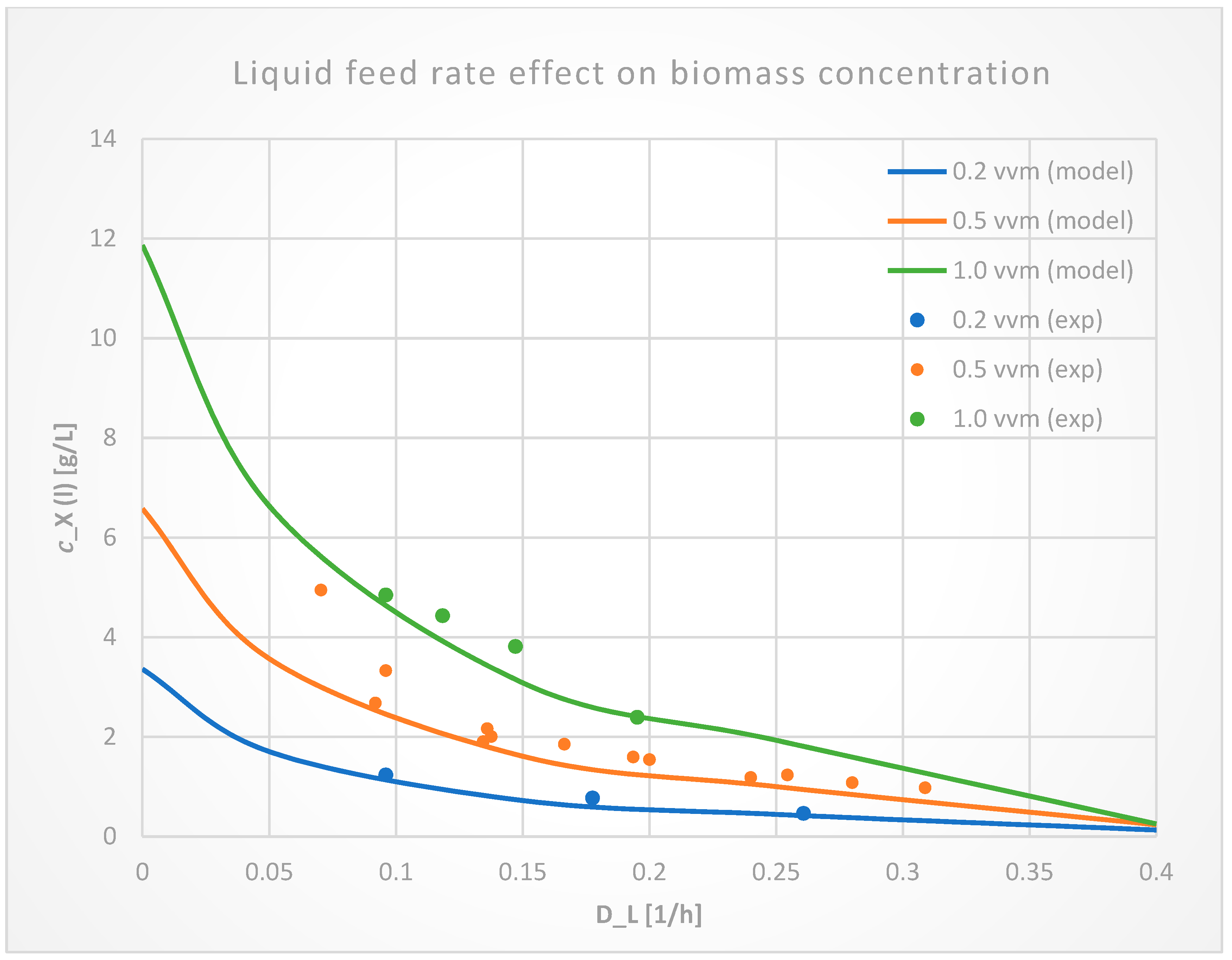
3.1.2. Liquid Flow Rate

$D_L$ in Figure 8 ranges from 0 to 0.4 1/h. This test was only conducted using the Schill setup for three different volumes and inflow rates of 0.2 vvm ($V=1.55 \mathrm{L}$), 0.5 vvm ($V=1.5 \mathrm{L}$), and 1.0 vvm ($V=1.4 \mathrm{L}$). Biomass concentration in both the model and experiment decreases as the liquid feed rate increases. The model appears to generate trends similar to experimented results, in spite of having differences. Model results are presented after reaching steady state, but based on the simulation results, the biomass concentration grows over time regardless of other substrates. Therefore, we could justify that the simulation time is the deterministic factor in the differences between the model and experiment values in this case.

Increasing the liquid feed rate causes a decrease in the biomass concentration due to a reduction in the cell residence time. This is because the increased feed rate decreases the amount of time the biomass spends in the reactor, as the biomass is washed out of the reactor more quickly. This, in turn, reduces the overall retention time of the biomass in the reactor and leads to a lower biomass concentration. Additionally, the increased feed rate may also lead to incomplete substrate utilization, as the microorganisms have less time to break down the substrate before it exits the reactor.

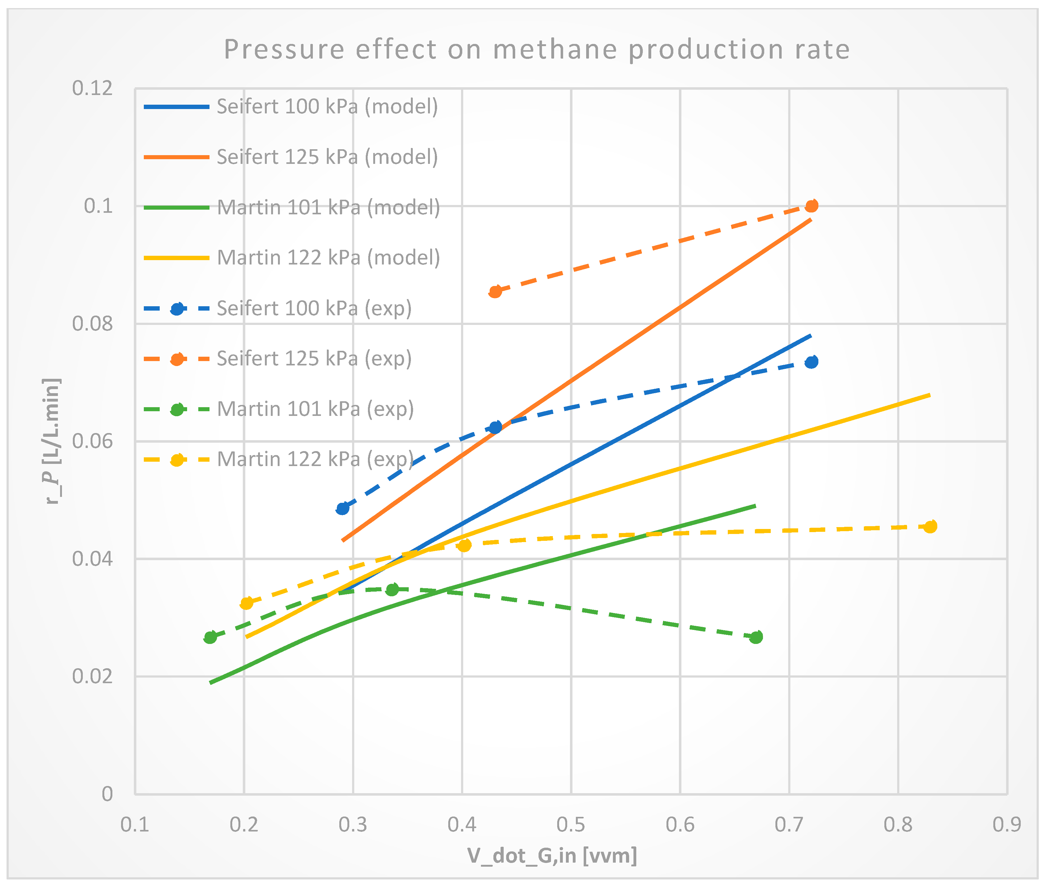
3.1.3. Reactor Overhead Pressure

Seifert at 100 and 125 kPa, and Martin at 101 and 122 kPa, investigated the effect of pressure on methane production rate. The effect can be seen in Figure 9, which compares their results with the model’s. Increasing the pressure has a positive effect on the reactor’s performance, according to both the experimental measurements of Seifert and Martin and the model. The model can appropriately forecast the ascending trends. The accuracy of the model for Seifert is more significant at higher gas inflow rates, whereas for Martin, the results are closer to the experimental values at lower ${\dot{V}}_{G,in}$ values.

By increasing the pressure in the reactor, the solubility and dissolution of gases in the liquid phase are increased. The increased concentration of gases in the liquid phase increases the rate of reaction, leading to higher conversion efficiency and increased methane production. Additionally, the increased pressure can improve the mass transfer of reactants into the microbial cells, allowing for higher methane production rates. Furthermore, elevated pressure can help maintain a stable pH and prevent the accumulation of volatile fatty acids, which can inhibit methanogenesis.

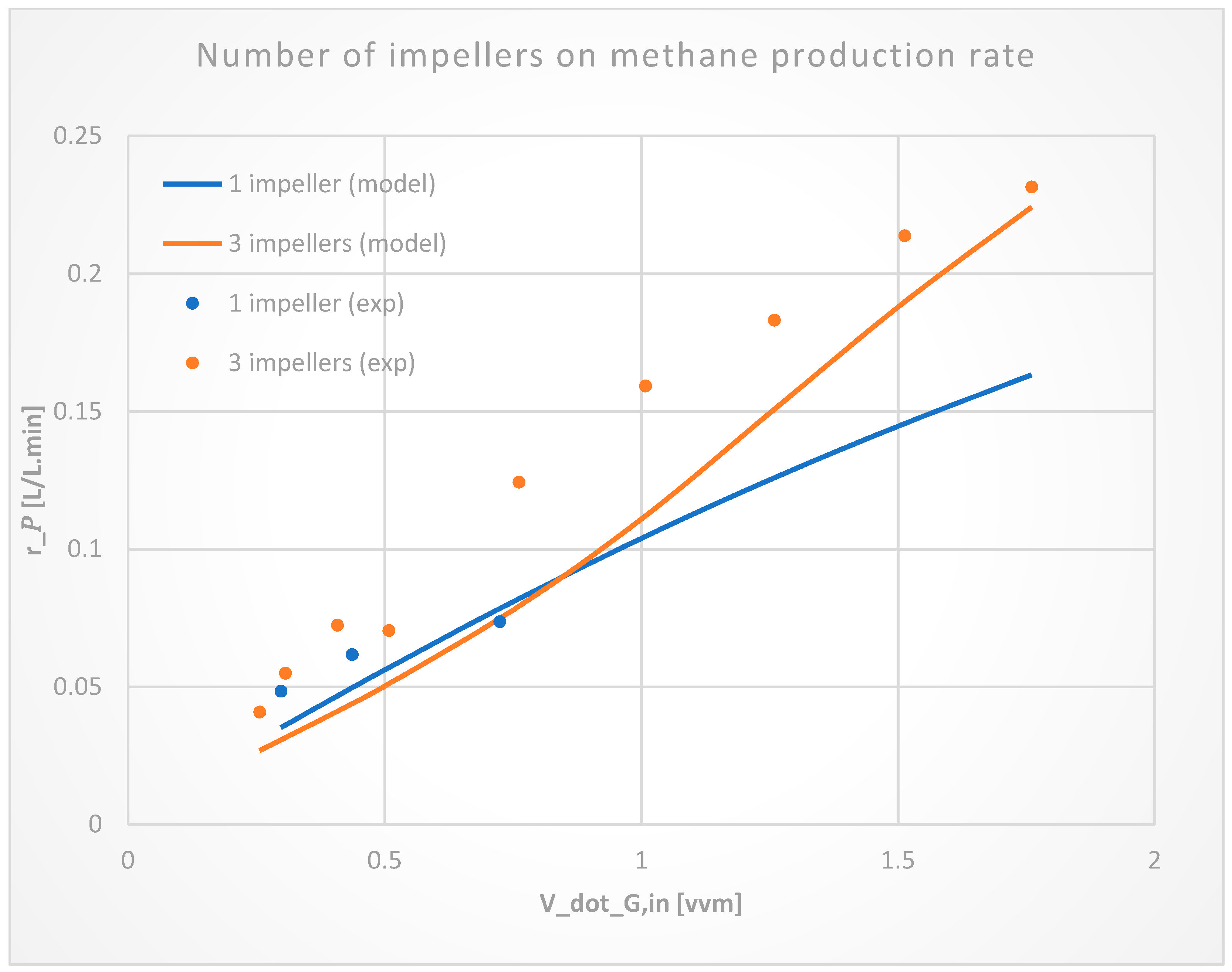
3.1.4. Number of Impellers

In order to obtain information about the effect of stirring regimes and reactor designs, and to improve the gas–liquid mass transfer, Seifert tested the experiment with two different active reactor volumes of $V=3.5\mathrm{L}$ and $V=5\mathrm{L}$ with two different impeller numbers of $n_{im}=1$ and $n_{im}=3$, respectively. In Figure 10, model results have been compared with the experimental values. According to the experiment, by increasing the number of impellers, methane production also increases. Meanwhile, based on the model, until ${\dot{V}}_{G,in}=0.83\mathrm{vvm}$, $r_P\left(l\right)$ is higher with one impeller than with three impellers, and after that, it is the opposite. Needless to say, the ascending trend of $r_P\left(l\right)$ as a function of ${\dot{V}}_{G,in}$ can be observed in both the model and experiment.

Increasing the number of impellers increases the dissipation energy $\epsilon$ and lowers the average bubble size $d_b$, resulting in higher interfacial area $a$, which would again end in higher gas–liquid mass transfer.

3.2. Sensitivity Analysis

To evaluate the effects of some of the influencing parameters of the experiments Schill et al. [12], Seifert et al. [8], and Martin et al. [14], a sensitivity analysis for all three cases was performed. To cover almost every aspect of the model (archaea reactions, absorption/desorption, reactor geometry, and axial mixing), the following parameters were selected: liquid recycle constant $\lambda$, impeller diameter $d_{im}$, reactor diameter $d_{re}$, axial mixing constants $b_1$ and $b_2$, biomass kinetics constants $k_D$, $m_X$, and ${\mu }^{max}$.

All the operating conditions and factors are the same as in the Results section, unless otherwise mentioned. To reach a complete steady-state for all the substrates in both gas and liquid phases, a simulation time of $t=100,000 \mathrm{s}\approx 28 \mathrm{h}$ for all the cases was determined. For each diagram, five simulations were performed, resulting in five nodes on each diagram, providing us with depicted trendlines. These nodes are the mean value of all the reactor cells of the corresponding parameter at the last time step.

3.2.1. Liquid Recycle Constant

Figure 11 demonstrates the effect of liquid recycle constant for two different values of $\lambda =0.5$ and $\lambda =0.75$ on methane concentration $c_P\left(g\right)$. The values of $c_P\left(g\right)$ with $\lambda =0.75$ are 0.57% in Schill, 0.98% in Seifert, and 0.54% in Martin, higher than with $\lambda =0.5$, which is almost negligible, and we could say that the fraction of liquid that we recycle to the inlet does not affect the methane concentration $c_P\left(g\right)$ considerably. Although this is true in our case, a more extensive study would be to investigate the minimum value of $\lambda$ that prevents a complete wash out of the biomass, since recycling is used to maintain the biomass in the reactor.

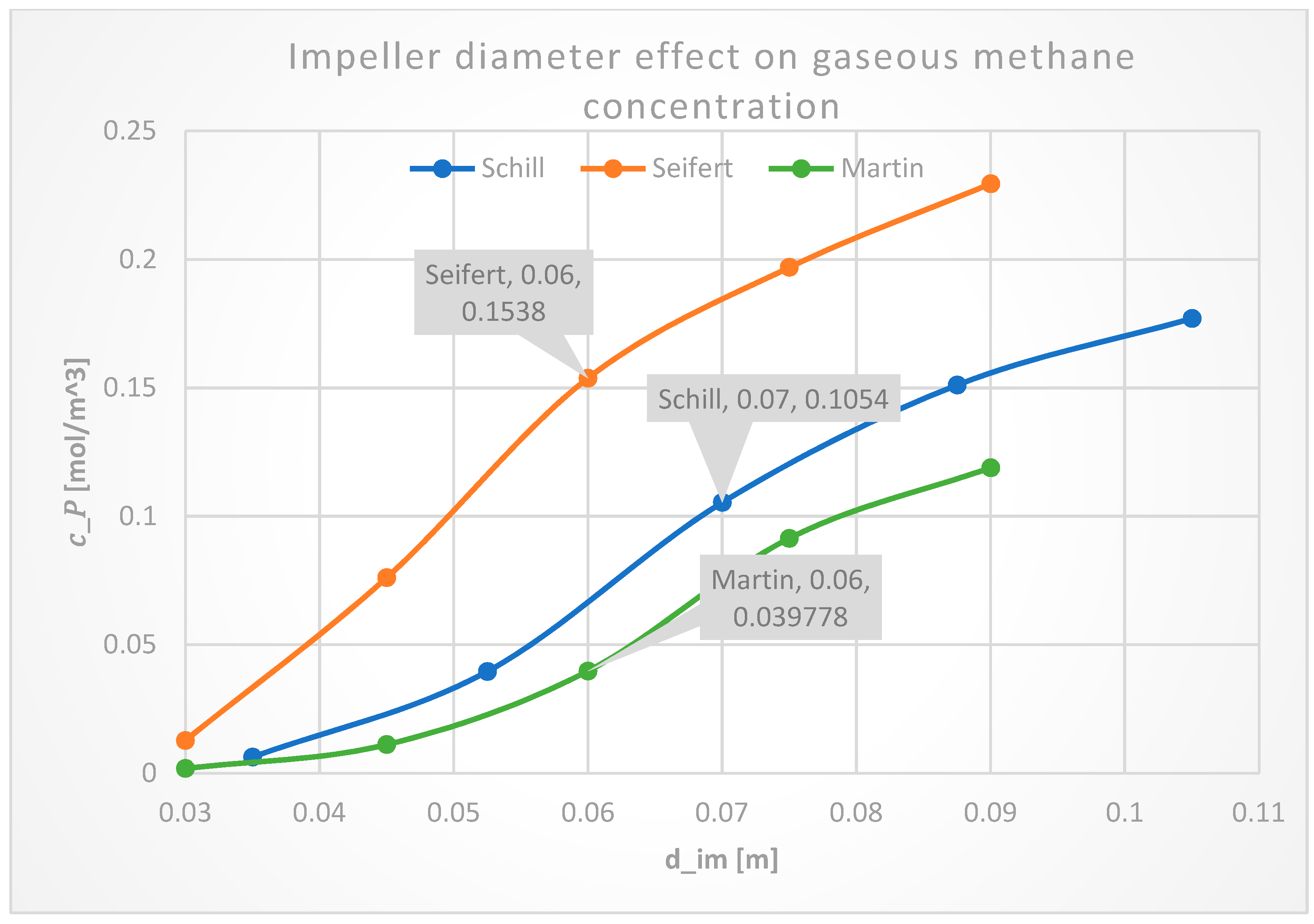
3.2.2. Impeller Diameter

Impeller diameter $d_{im}$ is set in a range of −50% to +50% of the experiments’ main impeller diameter described in Table 7. Figure 12 illustrates the effects of impeller diameter variations on $c_P\left(g\right)$. As you can see in all three cases, by lowering the impeller diameter, $c_P\left(g\right)$ also decreases, and by increasing it, $c_P\left(g\right)$ elevates. Methane concentration in gas phase $c_P\left(g\right)$ changes in Schill from −94.03% to 67.93% of the main concentration of 0.1054 $\mathrm{mol}·{\mathrm{m}}^{-3}$, in Seifert from −91.71% to 49.22% of the main concentration of 0.1538 $\mathrm{mol}·{\mathrm{m}}^{-3}$, and in Martin from −95.34% to 198.91% of the main concentration of 0.039778 $\mathrm{mol}·{\mathrm{m}}^{-3}$. The main impeller diameters and their corresponding methane concentrations, which are also the middle points, are tagged on the diagram.

$d_{im}$ directly influences the circulation and inter-stage numbers $N_{ci0}$ and $N_{is0}$, ungassed circulation and inter-stage liquid flow rates ${\dot{V}}_{L,ci0}$ and ${\dot{V}}_{L,is0}$, and also ungassed and stirring powers $P_{t0}$ and $P_t$. Needless to say, it plays an important role in the reactor performance, since it influences both the axial mixing and the gas–liquid mass transfer part of the model.

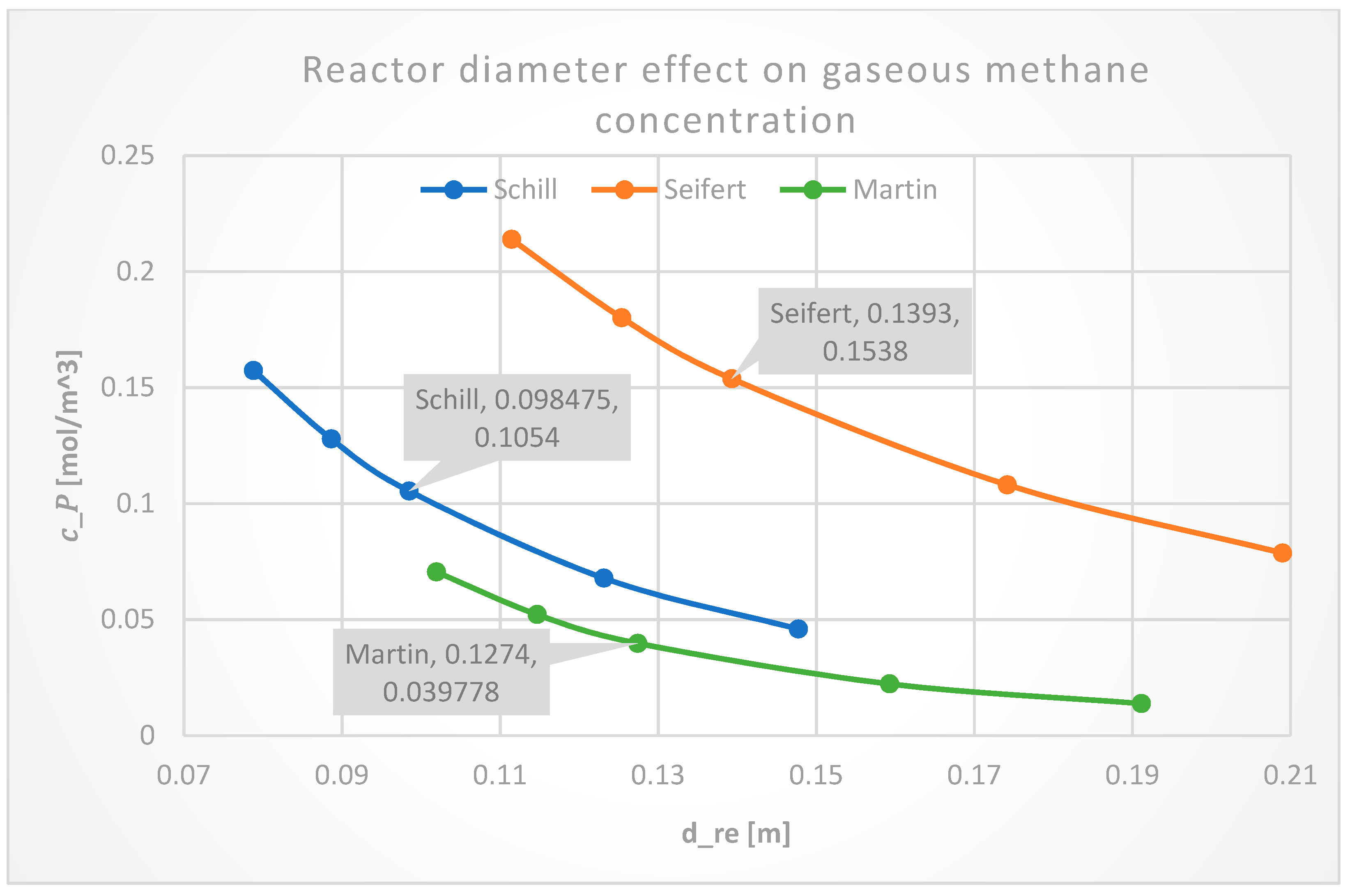
3.2.3. Reactor Diameter

Figure 13 demonstrates the effect of reactor diameter $d_{re}$ variations on $c_P\left(g\right)$. To prevent the impeller diameter $d_{im}$ exceeding the reactor diameter $d_{re}$ [11], $d_{re}$ ranges from −20% to +50% of the models’ main reactor diameter, which is calculated based on the reactor volume $V$ and the reactor height–diameter ratio $h:d_{re}$. These main diameters and their corresponding methane concentrations are shown on the diagram in the middle of the trendlines. With the variations of $d_{re}$, the reactor volume $V$ is kept constant. Opposite to $d_{im}$, in all three experiments, by reducing the reactor diameter (which also means higher reactor height), $c_P\left(g\right)$ increases, and by increasing it, $c_P\left(g\right)$ decreases. Methane concentration in gas phase $c_P\left(g\right)$ changes in Schill from 49.33% to −56.45% of the main concentration of 0.1054 $\mathrm{mol}·{\mathrm{m}}^{-3}$, in Seifert from 39.07% to −48.82% of the main concentration of 0.1538 $\mathrm{mol}·{\mathrm{m}}^{-3}$, and in Martin from 77.40% to −65.30% of the main concentration of 0.039778 $\mathrm{mol}·{\mathrm{m}}^{-3}$. Reactor diameter also affects both the axial mixing and the gas–liquid mass transfer part of the model.

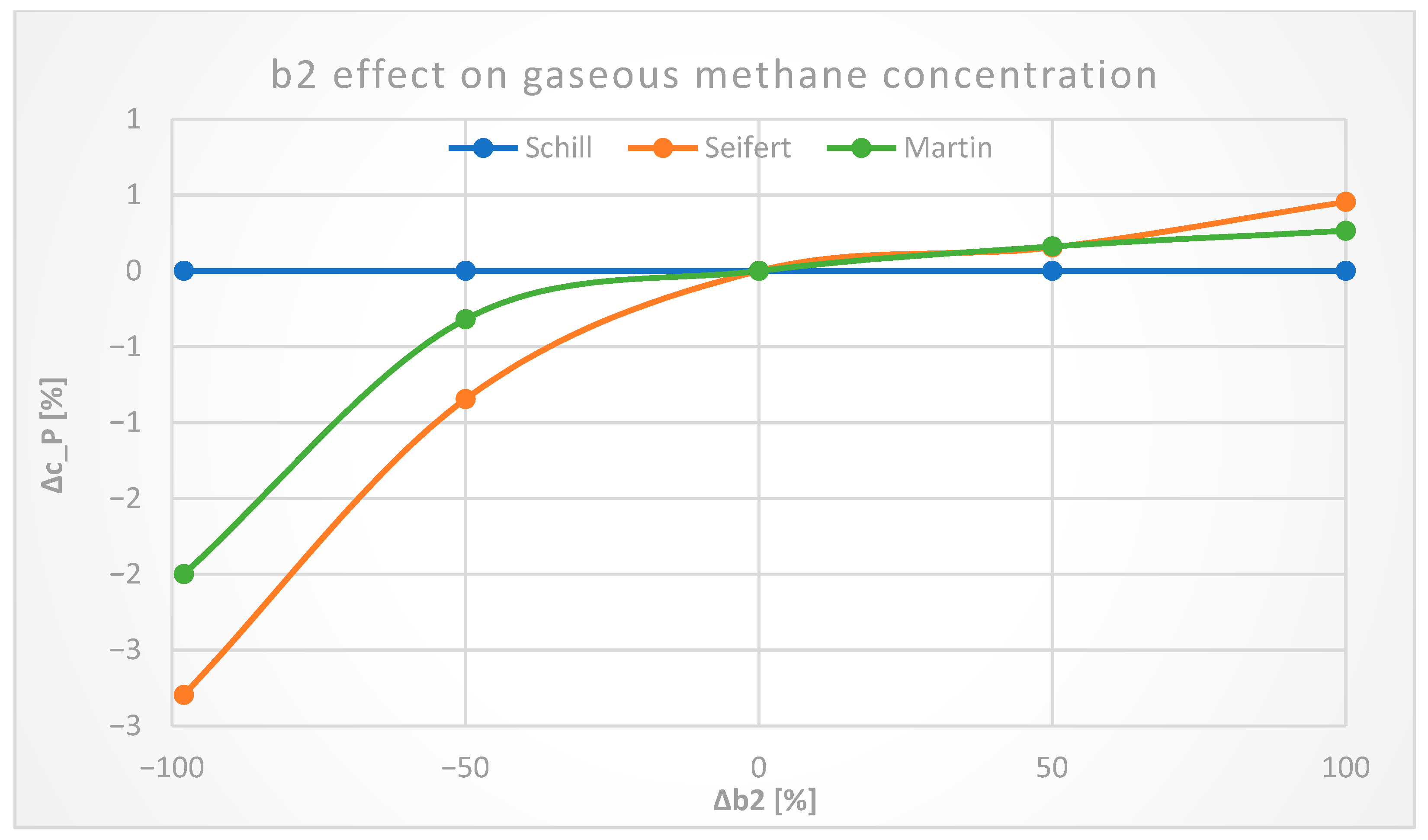
3.2.4. Axial Mixing Constants

Figure 14 and Figure 15 illustrate the variation effects of semi-empirical axial mixing constants $b_1$ and $b_2$ in Equations (30) and (31) on $c_P\left(g\right)$. They are varied from −98% to 100% of the main values $b_1=0.21$ and $b_2=0.236$. These constants are not that effective on methane concentration changes and almost negligible. Changes in $b_1$ cause $c_P\left(g\right)$ to change from about −11% to less than 7% in all three cases. Additionally, $b_2$ variations cause $c_P\left(g\right)$ to change from about −3% to less than 0.5% in Seifert and Martin, while having no effect in Schill.

Axial mixing constants are not exactly known and are only estimated in the model. They are not free parameters such as $d_{im}$ and $d_{re}$ that could be altered by changing the reactor geometry. Therefore, proving that $b_1$ and $b_2$ have insignificant effects through an uncertainty analysis indicates that even if they are not precisely measured, the reactor’s performance will not be substantially affected.

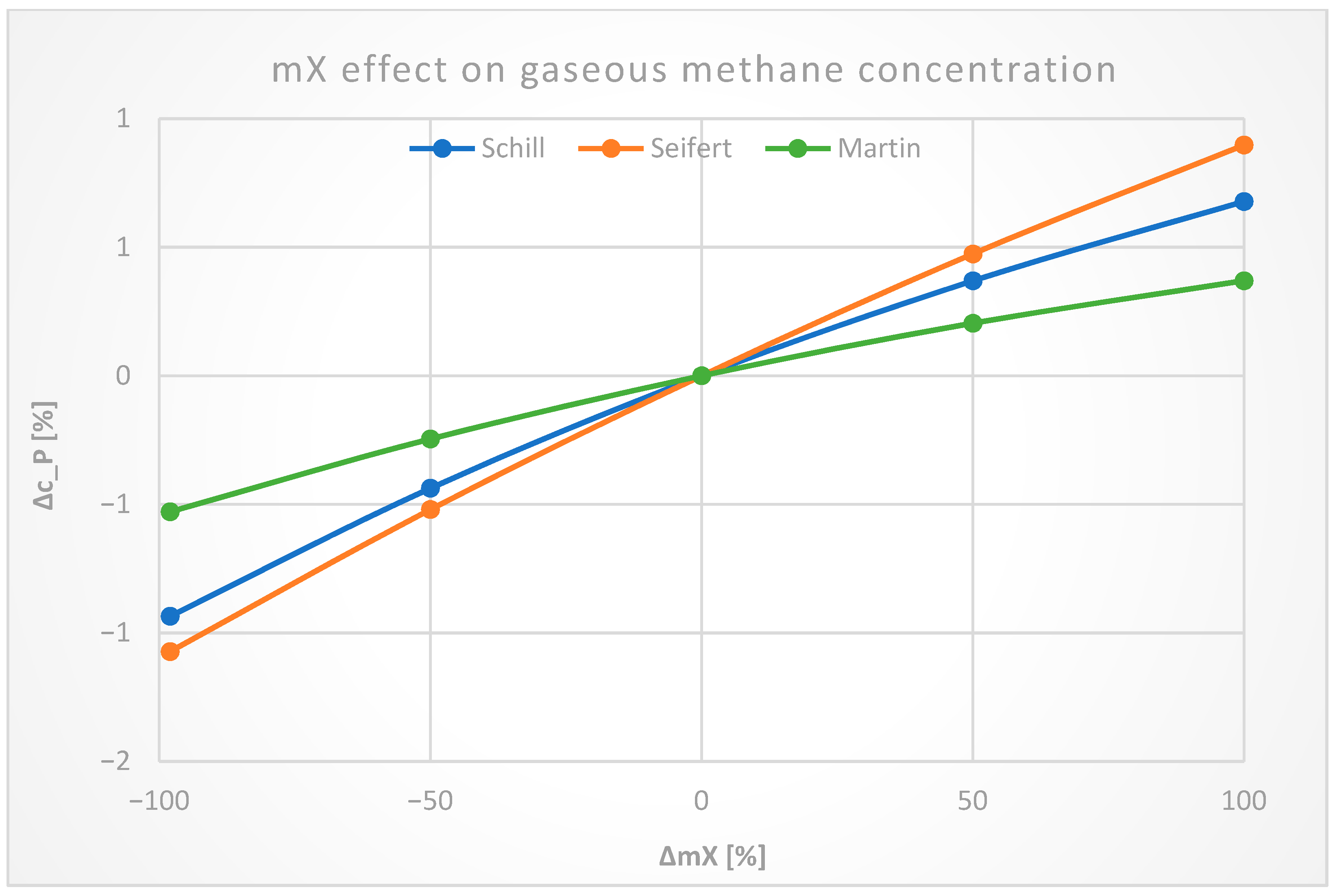
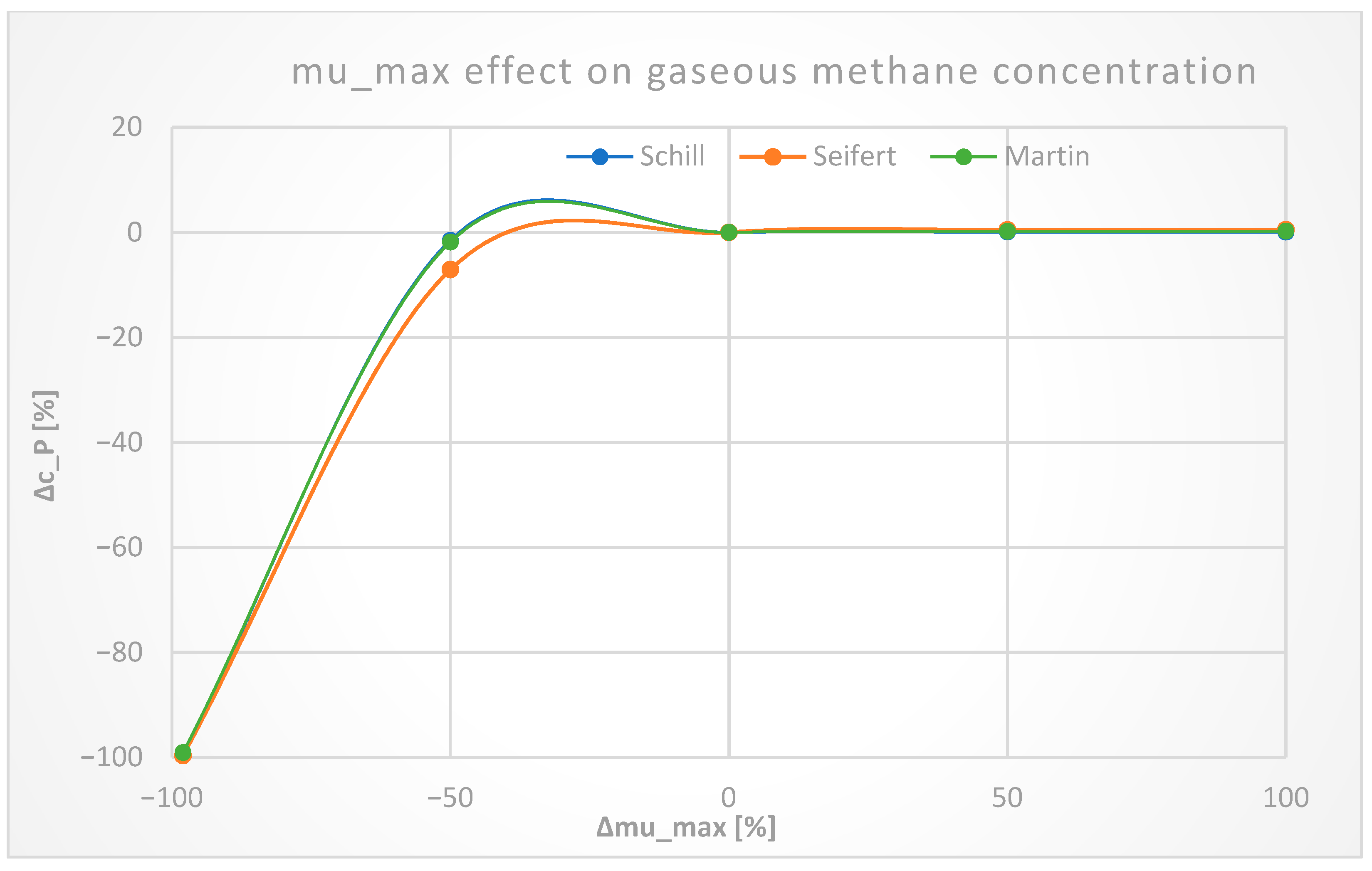
3.2.5. Biomass Kinetics Constants

Figure 16, Figure 17 and Figure 18 show the effects of biological kinetics constant changes in methane concentration. These parameters are ${\mathrm{H}}_2$ saturation constant $k_D=0.0056 \mathrm{mol}·{\mathrm{m}}^{-3}$, biomass maximum growth rate ${\mu }^{max}=0.00010028{\mathrm{s}}^{-1}$, and maintenance constant $m_X=0.00046389\mathrm{mol}·{\mathrm{mol}}^{-1}·{\mathrm{s}}^{-1}$. These parameters also range from −98% to 100% of the main values. $k_D$ changes cause $c_P\left(g\right)$ to vary within a range of −0.6% to 0.2%, and changes due to $m_X$ range from −1% to 0.9%. It is obvious that these parameters barely affect the performance of the reactor. The only exception is when ${\mu }^{max}$ is significantly lower than the liquid feed rate, which results in the elimination of the biomass and shuts down the operation; other than that, increasing it would result in only less than a 7% change in $c_P\left(g\right)$.

Generally, it is crucial to keep the liquid feed rate low enough to keep the reactor’s biomass intact if the system runs without liquid recycling. Similar to axial mixing constants, it is an advantage that $k_D$ and $m_X$ have minor impacts on the model’s efficiency, so their accuracy is not of much importance in the calculations. However, one has to bear in mind that ${\mu }^{max}$ should not be overestimated.

4. Discussion

As mentioned earlier, the initialization of $c_g$, $c_l$, $u_G$, and $u_L$ together was performed by Inkeri et al. [11], but in this study, it was decided to first initialize $c_g$ and $c_l$ and then calculate the velocities $u_G$ and $u_L$ after computing other parameters. Additionally, certain equations in Inkeri’s work were corrected. The effective cross-sectional area in Equation (8) was found to be $\left(1-{\varphi }_{\upsilon ,n}\right)A$ instead of $A$. Gas hold-up ${\varphi }_{\upsilon }$ was considered to account for the bubbles in the system while calculating the hydrostatic pressure using Equation (9) and the ideal gas pressure using Equation (10). To make the model more comprehensive, complementary equations for calculating pressure, density, viscosity, etc., were added. The final Equations (54)–(59) to be solved in MATLAB were presented at the end. The procedure of calculating the axial mixing coefficient $\Gamma$ was misguiding in the literature. Inkeri calculates everything inside each cell, yet $\Gamma$ is defined at the face of the cells. Therefore, a mean value approach of either circulation or inter-stage velocities to calculate $\Gamma$ was used depending on the position of the cells—inside, at the bottom, or at top of an impeller stage (Figure 5). It is worth mentioning that the more cells assumed for an impeller stage, the more accurate the calculations for the simulations would be. In Figure 7, the results of this study and Inkeri’s show no significant difference. However, for Schill and Seifert, the results of this study are closer to the experimental values for higher gas inflow rates. On the other hand, for Martin, the results of this study are more accurate for lower gas inflow rates and show a better fit compared to Inkeri’s results. Figure 8 demonstrates no remarkable differences between the results of this study and Inkeri’s for the liquid feed rate effect. The pressure effect in Figure 9 shows a significant improvement for both Seifert and Martin, which provides a more accurate demonstration of pressure effect compared to Inkeri. For the effect of the number of impellers in Figure 10, Inkeri’s study demonstrates a better fit to the experimental data with three impellers; although, with gas inflow rates higher than 1.5 vvm, this study shows closer values.

The inaccurate calculation of flow velocities in the reactor may be caused by the fact that the one-dimensional nature of the model did not account for radial effects of the system. This shortcoming could become more pronounced in large-sized industrial reactors, where mass transfer would not be well approximated by such a simple one-dimensional model. The effects of temperature and pH were not examined in this model. If the operating temperature is changed, all temperature-dependent parameters such as ${\mu }_g$, ${\mu }_L$, ${\rho }_L$, $D_g$, and $H_g$ should be adjusted accordingly. An alternative approach would be to express equations for these parameters as a function of $T$, rather than manually inserting them in the code. However, the validity of empirically obtained parameters must be assessed at different temperatures. According to Table 1, depending on the model’s requirements and operating conditions, pH can be maintained acidic or basic, fixed at a value or within a range not too far from 7.0. Furthermore, most cases were operated at a thermophilic range (55–65 °C). Based on Equation (45), the ammonia and water reaction rates can be computed to ensure mass balance for a more accurate modeling.

In the Results section, initially, simulation times were kept relatively short to provide a visual perception of how the concentration of substrates in the experiments developed over time and reactor height and to compare them with each other. Real-time simulations were attempted in the Model Validation and Sensitivity Analysis sections. Based on the literature, Schill et al. [12] conducted their experiments for approximately 25 hours, Seifert et al. [8] for 37 hours, and Martin et al. [14] for about 4 days. The liquid feed rates $D_L$ in Schill, Seifert, and Martin were $0.096{\mathrm{h}}^{-1}$, $0.05{\mathrm{h}}^{-1}$, and 0, respectively, for Model Validation. The methane production rates produced by the model were in SI units of $\left(\mathrm{mol}·{\mathrm{m}}^{-3}·{\mathrm{s}}^{-1}\right)$. To compare the results with the experiments, the methane density calculated using the ideal gas law was used to convert the units to $\left(\mathrm{mol}·{\mathrm{L}}^{-1}·{\min }^{-1}\right)$. Additionally, the units in Seifert were in $\left(\mathrm{mmol}·{\mathrm{L}}^{-1}·{\mathrm{h}}^{-1}\right)$, so the densities calculated by the model were also used to convert them. Although densities were almost the same for different gas inflow rates, it could have caused errors when comparing the results. Most of the experimental measurements were presented in diagram formats in the literature, so visually converting them into x–y coordinates could have created minor errors as well.

It was found during model validation and sensitivity analysis that methane concentration and production rate had a direct relationship with gas inflow rate ${\dot{V}}_{G,in}$, reactor overhead pressure $P_{re}$, number of impellers $n_{im}$, liquid recycle constant $\lambda$, and impeller diameter $d_{im}$. Although the difference between $\lambda =0.5$ and $\lambda =0.75$ was small, the effect of other (especially very small) lambda values was not checked. Meanwhile, liquid feed rate $D_L$ and reactor diameter $d_{re}$ showed an inverse relationship. $d_{im}$ and $d_{re}$ both had a significant impact on the reactor’s performance since they highly influenced gas–liquid mass transfer. On the other hand, axial mixing constants $b_1$ and $b_2$ and biomass kinetics constants $k_D$, ${\mu }^{max}$, and $m_X$ had negligible effects on methane production rate.

5. Conclusions

The most challenging issue in biological methanation is the gas–liquid mass transfer, which is mainly due to the low solubility of ${\mathrm{H}}_2$ in the archaea medium. Furthermore, releasing the reaction heat effectively is crucial for maintaining the chemical equilibrium of methanation [37]. Modeling is a widely used approach for enhancing and accelerating developments in this field, which allows for more reliable testing of various operational conditions and reactor designs beyond the experimental range. Hence, several fundamental and semi-fundamental modeling techniques have been employed in the BM literature to accurately estimate the reactor performance. Each approach focuses on a specific set of parameters depending on the model under investigation.

The dynamic model presented in this study, a 1-dimensional plug-flow model in a CSTR, integrates concepts for the gas–liquid mass transfer (absorption and desorption), methanogenic archaea growth kinetics, and reactor hydrodynamics (main and axial mixing flows). Despite the assumed values and mentioned uncertainties causing differences with experimental measurements, the developed MATLAB code was found to be valid compared to the literature data. The model enables us to adapt the constants for biological reactions for additional archaea cultures by utilizing culture-specific constants based on experimental values provided in the literature.

The sensitivity analysis results showed that the effect of liquid recycle constant λ on methane concentration $c_P\left(g\right)$ was almost negligible. The values of $c_P\left(g\right)$ with $\lambda =0.75$ were only 0.57% in Schill, 0.98% in Seifert, and 0.54% in Martin higher than with $\lambda =0.5$. Impeller diameter $d_{im}$ had a significant impact on $c_P\left(g\right)$, with methane concentration changing from −94.03% to 67.93% in Schill, −91.71% to 49.22% in Seifert, and −95.34% to 198.91% in Martin as $d_{im}$ was varied from −50% to +50% of the main impeller diameter. The reactor diameter $d_{re}$ also had a notable effect on $c_P\left(g\right)$, with methane concentration changing from 49.33% to −56.45% in Schill, 39.07% to −48.82% in Seifert, and 77.40% to −65.30% in Martin, as $d_{re}$ was varied from −20% to +50% of the main reactor diameter. However, the semi-empirical axial mixing constants $b_1$ and $b_2$ had almost negligible effects on methane concentration, with changes in $b_1$ causing $c_P\left(g\right)$ to change from about −11% to less than 7% and $b_2$ variations making $c_P\left(g\right)$ change from about −3% to less than 0.5% in Seifert and Martin. The biological kinetics constants $k_D$, ${\mu }^{max}$, and $m_X$ had relatively small effects on methane concentration, with $k_D$ changes causing $c_P\left(g\right)$ to vary within a range of −0.6% to 0.2% and changes due to $m_X$ ranging from −1% to 0.9%.

The results of this work show notable accuracy in lower gas inflow rates for Martin and higher gas inflow rates for Schill and Seifert compared to Inkeri’s results. Additionally, the results of this work demonstrate better accuracy in the pressure effect compared to Inkeri’s results. These improvements in accuracy could be attributed to the modifications made in this work compared to Inkeri’s study. However, despite the increasing quality of the model, we cannot yet adequately describe the discrepancies and the biological processes according to the current state of knowledge. Biological methanation being a novel approach still requires extensive research and improvement in the industrial scope. The following challenges could be considered to get closer to an ideal biological methanation system:

• Developing a model that considers the effects of parameters and operating conditions, such as pH, temperatures, and nutrients, simultaneously with reactor hydrodynamics, gas–liquid mass transfer, and microorganisms’ growth kinetics.
• Evaluating the possibilities of combining different reactor designs to achieve higher methane concentrations.
• Exploring novel technologies about more efficient ex situ bio-methanation, higher ${\mathrm{H}}_2$ solubility, decreasing bubble diameter $d_b$, and improving volumetric gas–liquid mass transfer coefficient $k_{L}a$.

References

1. Ellabban, O.; Abu-Rub, H.; Blaabjerg, F. Renewable Energy Resources: Current Status, Future Prospects and Their Enabling Technology. Renew. Sustain. Energy Rev. 2014, 39, 748–764. [Google Scholar] [CrossRef]
2. Tan, C.H.; Nomanbhay, S.; Shamsuddin, A.H.; Park, Y.-K.; Hernández-Cocoletzi, H.; Show, P.L. Current Developments in Catalytic Methanation of Carbon Dioxide—A Review. Front. Energy Res. 2022, 9, 795423. [Google Scholar] [CrossRef]
3. Guneratnam, A.J.; Ahern, E.; FitzGerald, J.A.; Jackson, S.A.; Xia, A.; Dobson, A.D.W.; Murphy, J.D. Study of the Performance of a Thermophilic Biological Methanation System. Bioresour. Technol. 2017, 225, 308–315. [Google Scholar] [CrossRef] [PubMed]
4. Cavicchioli, R. Archae—Timeline of the Third Domain. Nat. Rev. Microbiol. 2011, 9, 51–61. [Google Scholar] [CrossRef]
5. Wagner, I.D.; Wiegel, J. Diversity of Thermophilic Anaerobes. Ann. N. Y. Acad. Sci. 2008, 1125, 1–43. [Google Scholar] [CrossRef]
6. Hoekman, S.K.; Broch, A.; Robbins, C.; Purcell, R. CO2 Recycling by Reaction with Renewably-Generated Hydrogen. Int. J. Greenhouse Gas Control. 2010, 4, 44–50. [Google Scholar] [CrossRef]
7. Burkhardt, M.; Koschack, T.; Busch, G. Biocatalytic Methanation of Hydrogen and Carbon Dioxide in an Anaerobic Three-Phase System. Bioresour. Technol. 2015, 178, 330–333. [Google Scholar] [CrossRef]
8. Seifert, A.H.; Rittmann, S.; Herwig, C. Analysis of Process Related Factors to Increase Volumetric Productivity and Quality of Biomethane with Methanothermobacter Marburgensis. Appl. Energy 2014, 132, 155–162. [Google Scholar] [CrossRef]
9. Shin, H.C.; Ju, D.-H.; Jeon, B.S.; Choi, O.; Kim, H.W.; Um, Y.; Lee, D.-H.; Sang, B.-I. Analysis of the Microbial Community in an Acidic Hollow-Fiber Membrane Biofilm Reactor (Hf-MBfR) Used for the Biological Conversion of Carbon Dioxide to Methane. PLoS ONE 2015, 10, e0144999. [Google Scholar] [CrossRef]
10. Rittmann, S.; Seifert, A.; Herwig, C. Essential Prerequisites for Successful Bioprocess Development of Biological CH4 Production from CO2 and H2. Crit. Rev. Biotechnol. 2015, 35, 141–151. [Google Scholar] [CrossRef]
11. Inkeri, E.; Tynjälä, T.; Laari, A.; Hyppänen, T. Dynamic One-Dimensional Model for Biological Methanation in a Stirred Tank Reactor. Appl. Energy 2018, 209, 95–107. [Google Scholar] [CrossRef]
12. Schill, N.; van Gulik, W.M.; Voisard, D.; von Stockar, U. Continuous Cultures Limited by a Gaseous Substrate: Development of a Simple, Unstructured Mathematical Model and Experimental Verification with Methanobacterium Thermoautotrophicum. Biotechnol. Bioeng. 1996, 51, 645–658. [Google Scholar] [CrossRef]
13. Díaz, I.; Pérez, C.; Alfaro, N.; Fdz-Polanco, F. A Feasibility Study on the Bioconversion of CO2 and H2 to Biomethane by Gas Sparging through Polymeric Membranes. Bioresour. Technol. 2015, 185, 246–253. [Google Scholar] [CrossRef] [PubMed]
14. Martin, M.R.; Fornero, J.J.; Stark, R.; Mets, L.; Angenent, L.T. A Single-Culture Bioprocess of Methanothermobacter Thermautotrophicus to Upgrade Digester Biogas by CO2-to-CH4 Conversion with H2. Archaea 2013, 2013, e157529. [Google Scholar] [CrossRef]
15. Savvas, S.; Donnelly, J.; Patterson, T.; Chong, Z.S.; Esteves, S.R. Biological Methanation of CO2 in a Novel Biofilm Plug-Flow Reactor: A High Rate and Low Parasitic Energy Process. Appl. Energy 2017, 202, 238–247. [Google Scholar] [CrossRef]
16. Rusmanis, D.; O’Shea, R.; Wall, D.M.; Murphy, J.D. Biological Hydrogen Methanation Systems—An Overview of Design and Efficiency. Bioengineered 2019, 10, 604–634. [Google Scholar] [CrossRef]
17. Luo, G.; Angelidaki, I. Integrated Biogas Upgrading and Hydrogen Utilization in an Anaerobic Reactor Containing Enriched Hydrogenotrophic Methanogenic Culture. Biotechnol. Bioeng. 2012, 109, 2729–2736. [Google Scholar] [CrossRef]
18. Bernacchi, S.; Rittmann, S.; Seifert, A.H.; Krajete, A.; Herwig, C.; Bernacchi, S.; Rittmann, S.; Seifert, A.H.; Krajete, A.; Herwig, C. Experimental Methods for Screening Parameters Influencing the Growth to Product Yield (Y(x/CH4)) of a Biological Methane Production (BMP) Process Performed with Methanothermobacter Marburgensis. AIMS Bioeng. 2014, 1, 72–87. [Google Scholar] [CrossRef]
19. Alitalo, A.; Niskanen, M.; Aura, E. Biocatalytic Methanation of Hydrogen and Carbon Dioxide in a Fixed Bed Bioreactor. Bioresour. Technol. 2015, 196, 600–605. [Google Scholar] [CrossRef]
20. Rachbauer, L.; Voitl, G.; Bochmann, G.; Fuchs, W. Biological Biogas Upgrading Capacity of a Hydrogenotrophic Community in a Trickle-Bed Reactor. Appl. Energy 2016, 180, 483–490. [Google Scholar] [CrossRef]
21. Coker, A.K. Chapter 21—Industrial and Laboratory Reactors—Chemical Reaction Hazards and Process Integration of Reactors. In Ludwig’s Applied Process Design for Chemical and Petrochemical Plants (Fourth Edition); Coker, A.K., Ed.; Gulf Professional Publishing: Boston, MA, USA, 2015; pp. 1095–1208. [Google Scholar] [CrossRef]
22. Wilke, C.R. A Viscosity Equation for Gas Mixtures. J. Chem. Phys. 1950, 18, 517–519. [Google Scholar] [CrossRef]
23. The Engineering Toolbox. Available online: https://www.engineeringtoolbox.com/gases-absolute-dynamic-viscosity-d_1888.html (accessed on 16 December 2022).
24. Garcia-Ochoa, F.; Gomez, E. Theoretical Prediction of Gas–Liquid Mass Transfer Coefficient, Specific Area and Hold-up in Sparged Stirred Tanks. Chem. Eng. Sci. 2004, 59, 2489–2501. [Google Scholar] [CrossRef]
25. Mazzeo, L.; Signorini, A.; Lembo, G.; Bavasso, I.; Di Palma, L.; Piemonte, V. In Situ Bio-Methanation Modelling of a Randomly Packed Gas Stirred Tank Reactor (GSTR). Processes 2021, 9, 846. [Google Scholar] [CrossRef]
26. Vasconcelos, J.M.T.; Alves, S.S.; Barata, J.M. Mixing in Gas-Liquid Contactors Agitated by Multiple Turbines. Chem. Eng. Sci. 1995, 50, 2343–2354. [Google Scholar] [CrossRef]
27. Schmitz, K.S. Chapter 5—Thermodynamics of the Liquid State. In Physical Chemistry; Schmitz, K.S., Ed.; Elsevier: Boston, MA, USA, 2017; pp. 203–260. [Google Scholar] [CrossRef]
28. Sander, R. Compilation of Henry’s Law Constants (Version 4.0) for Water as Solvent. Atmos. Chem. Phys. 2015, 15, 4399–4981. [Google Scholar] [CrossRef]
29. The Engineering Toolbox. Available online: https://www.engineeringtoolbox.com/diffusion-coefficients-d_1404.html (accessed on 17 December 2022).
30. Michel, B.J.; Miller, S.A. Power Requirements of Gas-Liquid Agitated Systems. AIChE J. 1962, 8, 262–266. [Google Scholar] [CrossRef]
31. Nienow, A.W. Gas–liquid mixing studies: A comparison of Rushton turbines with some modern impellers. Chem. Eng. Res. Des. 1996, 74, 417–423. [Google Scholar]
32. Bhavaraju, S.M.; Russell, T.W.F.; Blanch, H.W. The Design of Gas Sparged Devices for Viscous Liquid Systems. AIChE J. 1978, 24, 454–466. [Google Scholar] [CrossRef]
33. Fardeau, M.-L.; Peillex, J.-P.; Belaïch, J.-P. Energetics of the Growth of Methanobacterium Thermoautotrophicum and Methanococcus Thermolithotrophicus on Ammonium Chloride and Dinitrogen. Arch. Microbiol. 1987, 148, 128–131. [Google Scholar] [CrossRef]
34. Chezeau, B.; Vial, C. Chapter 19—Modeling and Simulation of the Biohydrogen Production Processes. In Biohydrogen, 2nd ed.; Biomass, Biofuels, Biochemicals; Pandey, A., Mohan, S.V., Chang, J.-S., Hallenbeck, P.C., Larroche, C., Eds.; Elsevier: Amsterdam, The Netherlands, 2019; pp. 445–483. [Google Scholar] [CrossRef]
35. MathWorks. Available online: https://uk.mathworks.com/company/newsletters/articles/stiff-differential-equations.html (accessed on 17 December 2022).
36. MathWorks. Available online: https://uk.mathworks.com/help/matlab/ref/ode15s.html (accessed on 17 December 2022).
37. Eggers, N.; Böttger, J.N.J.; Kerpen, L.; Sankol, B.U.; Birth, T. Refining VDI Guideline 4663 to Evaluate the Efficiency of a Power-to-Gas Process by Employing Limit-Oriented Indicators. Energy Effic. 2021, 14, 73. [Google Scholar] [CrossRef]
Figure 1. Gas and liquid inlet and outlets, absorption and desorption of the reactants and products alongside the biomass growth.
Processes 11 01510 g001
Figure 2. Flowchart of the model.
Processes 11 01510 g002
Figure 3. (a) Dimensions of the example reactor with impellers, (b) spatial discretization, gas, and liquid inlet and outlets with liquid recycling schematic.
Processes 11 01510 g003
Figure 4. Diffusion modeling inside the reactor.
Processes 11 01510 g004
Figure 5. (a) a node in the interior of the impeller stage, (b) a node at the bottom of the stage, and (c) a node at the top of the stage.
Processes 11 01510 g005
Figure 6. CH 4 ( g ) , CO 2 ( g ) , H 2 ( g ) , and biomass (l) concentration comparison of the three cases.
Processes 11 01510 g006
Figure 7. Model prediction of methane production rate r P ( l ) as a function of gas inflow rate V ˙ G , i n vs. the three experiments.
Processes 11 01510 g007
Figure 8. Model prediction of biomass concentration c X ( l ) as a function of liquid flow rate D L vs. Schill’s experimental data for three gas inflow rates V ˙ G , i n .
Processes 11 01510 g008
Figure 9. Model prediction of methane production rate r P ( l ) as a function of gas inflow rate V ˙ G , i n vs. the measured data of Seifert and Martin for two reactor overhead pressures P r e .
Processes 11 01510 g009
Figure 10. Model prediction of methane production rate r P ( l ) as a function of gas inflow rate V ˙ G , i n vs. Seifert’s experimental data for two different impeller numbers n i m .
Processes 11 01510 g010
Figure 11. Model predictions of gaseous methane concentration c P ( g ) as a function of gas inflow rate V ˙ G , i n for two different liquid recycle constants λ .
Processes 11 01510 g011
Figure 12. Model predictions of gaseous methane concentration c P ( g ) as a function of impeller diameter d i m .
Processes 11 01510 g012
Figure 13. Model predictions of gaseous methane concentration c P ( g ) as a function of reactor diameter d r e .
Processes 11 01510 g013
Figure 14. Model predictions of gaseous methane concentration c P ( g ) change as a function of the b 1 change in the three cases.
Processes 11 01510 g014
Figure 15. Model predictions of gaseous methane concentration c P ( g ) change as a function of the b 2 change in the three cases.
Processes 11 01510 g015
Figure 16. Model predictions of gaseous methane concentration c P ( g ) change as a function of the hydrogen saturation constant k D change in the three cases.
Processes 11 01510 g016
Figure 17. Model predictions of gaseous methane concentration c P ( g ) change as a function of the maintenance constant m X change in the three cases.
Processes 11 01510 g017
Figure 18. Model predictions of gaseous methane concentration c P ( g ) change as a function of the biomass maximum growth rate μ m a x change in the three cases.
Processes 11 01510 g018