Abstract
The rise of artificial intelligence (AI)-based image analysis has led to novel application possibilities in the field of solvent analytics. Using convolutional neural networks (CNNs), better and more automated analysis of optically visible phenomena becomes feasible, broadening the spectrum of non-invasive measurements. These so-called smart sensors have attracted increasing attention in pharmaceutical and chemical process engineering; their additional sensor data enables more precise process control as additional process parameters can be monitored. This contribution presents an approach to analyzing single rising droplets to determine their physical properties; for example, geometrical parameters such as diameter, projection area and volume. Additionally, the rising velocity is determined, as well as the density and interfacial tension of the rising liquid droplet, determined from the force balance. Thus, a method was developed for analyzing liquid–liquid properties suitable for real-time applications. Here, the size range of the investigated droplet diameters lies between 0.68 mm and 7 mm with an accuracy for AI detecting droplets of ±4 µm. The obtained densities lie between 0.822 kg·m−3 for rising n-butanol droplets and 0.894 kg·m−3 for toluene droplets. For the derived parameters, such as the interfacial tension estimation, all of the data points lie in a range from 12.75 mN·m−1 to 15.25 mN·m−1. The trueness of the investigated system thus is in a range from −1 to +0.4 mN·m−1, with a precision of ±0.3 to ±0.6 mN·m−1. For density estimation using our system, a standard deviation of 1.4 kg m−3 from the literature was determined. Using camera images in conjunction with image analysis improved by artificial intelligence algorithms, combined with using empirical mathematical formulas, this article contributes to the development of easily accessible, cheap sensors.
1. Introduction
Online process supervision enabled by a digital camera is a cheap and simple method to rapidly gain more insight into the process parameters of various chemical substances in liquid form and can be seen as a smart sensor [1]. Applying an AI-based evaluation, a smart camera sensor is built to work continuously and evaluate the data automatically. Particularly, multiphase transport processes can benefit from modern sensor technology [2,3]. Together with the growing interest in continuous processes, the miniaturization and modularization of smart sensors are on the rise. [4,5] Many tools and methods in the framework of Industry 4.0 form a new industrial revolution, in which attempts are made to further automate processes [6]. Among other applications, numerical algorithms are assisting automation processes which are summarized under the term AI, with a subcategory of deep learning (DL). For image classification, an artificial neural network (ANN) can be used to recognize features of object classes and learn to distinguish them from others, and ideally, then apply these features to unseen data [7]. Among other fields, DL has been applied in medical technology in the image recognition of cancer cells and the vehicle design of self-driving cars [3,8].
The chemical industry has shown interest in the progress made in data-driven computational methods and the potential benefits that machine learning (ML) and artificial intelligence could bring. ML is a process that utilizes historical data to generate algorithms for performing various tasks, and it has gained popularity in the process industry due to the increase in available data and computational power. AI applications in the chemical industry are diverse, ranging from active learning for recognizing steps in chemical batch production [6] to computer vision for process monitoring. Image processing is also being used for tasks such as object localization and segmentation, with applications in measuring abrasion [9], reading analog gauges and identifying thermal anomalies using Boston Dynamics’ dog-like robot inspection method in industrial facilities [8]. Additionally, deep learning is being used for defect detection in quality control, which leads to improved performance and cost reduction through process automation [6,10,11]. Further examples are the combination of ANN methods with capacitive sensors to investigate two-phase homogenous fluids [12] or the use of CNNs in fermentation systems [13].
Some process variables cannot be measured online directly without the help of sensors. Nevertheless, in some cases especially, these variables are needed to ensure safety and product quality. Computational sensors called soft sensors can infer respective values, use knowledge or measurements to predict quality variables and can provide appropriate remedies [6,7]. This work presents an approach to measure the densities, interfacial tensions and additional geometrical data of rising droplets using AI-based image segmentation. Geometrical data refers to the area, diameter, volume and aspect ratio of an uprising droplet. This method enables a cheap and fast online measurement of these parameters for process control and research applications.
In this work, single droplets are generated, rising in a continuous liquid. The rising droplet is observed by a digital camera, and the images are analyzed by an AI algorithm to determine their geometric properties. Moreover, by iteratively solving a force balance, different physical properties such as density and interfacial tension can be calculated. The sensor presented in this work can be applied to different setups due to its non-invasive and optical characteristics. The model was developed in the scope of the KEEN project that investigates the application possibilities of Artificial Intelligence methods in the process industry (http://keen-plattform.de/keen/en/ (accessed on 31 March 2023)). Within the project scope, it can be coupled to investigate the composition of a raffinate stream leaving an extraction column. The contribution is structured as follows: After the abstract and introduction of the topic, the utilized materials and methods are presented in Section 2. Here, the experimental setup with the used chemicals is presented first, followed by data analysis, where an image analysis using artificial intelligence and its metrics is presented. In the results section, the AI algorithm is evaluated in terms of its accuracy in detecting droplets. This is followed by the evaluation of the rising velocity experimentally compared to mathematical equations such as flow resistance and drag coefficient evaluation. Finally, the obtained density and interfacial tension are described. The results are followed by a “conclusion and further work” section.
2. Materials and Methods
This section describes the materials used, such as chemicals, and the experimental setup for the main evaluation in Section 2.1, followed by the related data evaluation in Section 2.2.
2.1. Experimental Setup
Rising droplet experiments are carried out in an extraction cell (Vint = 17 mL) made of glass which is surrounded by a glass chamber. The inner diameter of the cell is 15 mm. The glass chamber and the heating jacket of the extraction cell were filled with water to reduce optical effects in the videos and images. In total, three glass nozzles with different and initially unknown inner diameters (at the top) were used (determination of the inner diameters made using micro-computed tomography—see Data Availability Statement). Images of the experimental setup and a sketch of the setup are shown in Figure 1.
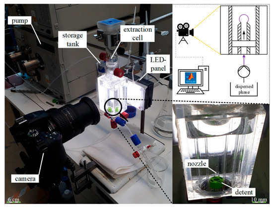
Figure 1.
Experimental setup including extraction cell, camera, LED panel and pump.
The three investigated nozzles are 80 mm in length, and on the bottom side, they have an outer diameter of 6 mm and an inner diameter of 1.2 mm. The nozzle is inserted at the bottom of the extraction cell and adjusted by a 3D printed polymer grid to ensure exact orientation in the tube and uniform wall effects on the droplets. The nozzle is connected with the pump by a tube which is inserted directly into the bottom of the nozzle. The dual piston pump Dynamax SD-1 by Rainin (today: Agilent Technologies) feeds the dispersed phase from the storage tank through the nozzle into the extraction cell.
To complete the experimental setup, an LED panel is placed behind the extraction cell to ensure sufficient illumination. The panel is combined with a screen of frosted glass and two layers of white photographic paper to enhance light scattering. The camera is placed in front of the cell at a distance of approx. 5 cm. Its frame rate is set to 24 s−1 while the image resolution is set to 1920 × 1080 pixels for video recording.
The Morton number is a dimensionless number used together with the Eötvös number or Bond number to characterize the shape of bubbles or drops moving in a surrounding fluid or continuous phase.
The Morton number, , is a measure for the ratio of viscous forces to surface forces and depends only on liquid parameters and gravity. As long as these liquid parameters do not vary due to variables such as temperature variations, the Morton number is a constant [14].
The pure chemical substances used, their interfacial tension and their number are displayed in Table 1.

Table 1.
Surface tension and Mo number of typical liquid–liquid systems at 20 °C.
The interfacial tension refers to mechanical stresses and thus forces that occur at the boundary between two different phases that are in contact with each other. The investigation of dual systems of different chemical compositions is therefore interesting. Moreover, we expect the uprising droplets of a mixture of toluene/n-butyl acetate of unknown composition to lie somewhere in the middle of the values of the pure components.
2.2. Droplet Segmentation Using CNNs
A convolutional neural network is a subcategory of artificial neural networks. CNNs are created to process data with a grid-like topology, such as time series data or images [4]. In general, neural networks are built of numerous computational units called perceptrons. A simple representation of one perceptron is shown in Figure 2.
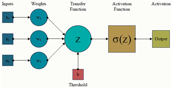
Figure 2.
Basic functionality of an artificial neuron.
A perceptron takes multiple inputs and produces one output. Within the transfer function z, the inputs and weights are combined with another parameter representing the threshold or bias b [5].
Depending on the value of the threshold , the perceptron either outputs 1 or 0. If the threshold is extremely small, it is easy for the perceptron to produce 1 as an output. This is the simplest form of such computational units (depicted in Figure 2).
An artificial neural network is composed of multiple layers in which the neurons are arranged. Overall, a neural network consists of an input layer, an output layer and at least one hidden layer in between. From the output of the last layer in the neural network, an error is calculated, which describes the difference between the output value and the true value. The error is described by the so-called cost function. During the training, the weights and biases are changed accordingly so that the resulting error becomes as small as possible [15]. The workflow to start with the training is depicted in Figure 3.
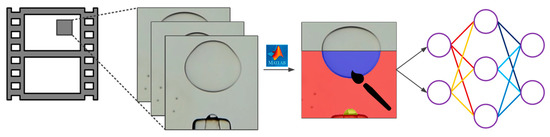
Figure 3.
Recorded videos of the rising droplets are cut into frames. These frames are then manually labeled using Matlab’s Image Labeler tool. This means every pixel is assigned one of three classes: background (red color), attached droplet to the nozzle (yellow) or detached droplet (blue).
Recorded videos of the process are cut into frames. These frames are then manually labeled using Matlab’s Image Labeler tool. This means every pixel in the image is assigned one of three classes: background (indicated by red color), attached droplet to the nozzle (indicated by yellow color) or detached droplet (indicated by blue color). This pixelwise annotation of an image is called image segmentation. The images and their segmentation masks, consisting of one of three labels for every pixel in the image, are used to train the convolutional neural network in Matlab. For the training, a dataset of 970 labeled pictures with a resolution of 224 × 224 pixels are used. Since the pre-trained CNN must be suitable for segmentation tasks, a ResNet-50 is used. Data augmentation is also applied to artificially enlarge the training set and thus make the network more robust. The specific augmentation parameters are depicted in Table 2.
Table 2.
Data augmentation settings during CNN training.
The reflection of the pictures on the X-axis, as well as the Y-axis, is performed. Moreover, a random rotation of −20° to +20° and symmetric scaling are applied to the pictures during training. The ResNet-50 is training for 31 epochs with a mini batch size of 4 using Matlab 2020b on a Nvidia GeForce GTX 1660 Ti Max-Q graphics card. Training takes 90 s/epoch on the GPU, resulting in 46.5 min total training time. The computational time per image for classification is 0.37 s.
3. Results
This section first deals with the accuracy of the image processing method using the CNN. It is then followed by the estimation of the rising velocity, the drag coefficient, the density of the uprising droplet and the interfacial tension. The respective pseudocode can also be found in the appendix (see Appendix A.1).
3.1. Accuracy of CNN for Droplet Projection Area
The metrics applied to determine the measurement error of the AI algorithm are as follows. They are measured using the validation data set consisting of eight images. TP stands for true positive, where positive cases are identified as positive; true negatives as TN, where negative cases are identified as negative; false positives as FP, where negative cases are identified as positive and false negatives as FN, where positive cases are identified as negative. For example, when a pixel assigned to the class “background” is detected as “detached droplet”, this would be a false negative.
The trained network reaches a mean segmentation accuracy (Recall) of 99.5% on the validation data and 99.63% on the training data, see Table 3. This translates to 477 wrongly labeled pixels out of 50,176 pixels in total (224 × 224 pixel image) on a single validation image. Additionally, the accuracy of 99.3% and precision score of 99.8% indicate a low failure rate for the neural network. As the Dice coefficient of 97.7% and the F1 contour of 97.8% matching score are the lowest scores, this already indicates that the biggest deviations of the network can be found on the contour lines of the different detected objects. This is an indicator of the very good generalization ability of the trained ResNet50 as the main areas of the different objects are detected highly accurately. A more graphic conception of this result is a line with a thickness of 1 pixel around the boundary of the originally labeled droplet, as depicted in Figure 4.
Table 3.
Segmentation performance indicators of the CNN training.
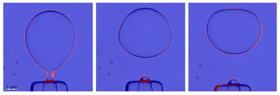
Figure 4.
Representation of incorrectly identified pixels by the ResNet50 by an overlay of the correct (blue) and wrong (red) detected pixels over the original image.
From the visual analysis of the images, the prediction, based on the segmentation parameters, that the deviations mainly occur at the contour lines of the droplets can be confirmed. Moreover, a big portion of misdetections occurs on sticking droplets; therefore, the result for the detached droplets is even better than expected. This is very beneficial for the post-processing routine as it relies mainly on the accurate segmentation of the detached droplets.
In summary, it can be stated that the performance of the ResNet50 is already at a very high level. The overall performance is good (±2 px), with the AI-assisted segmentation typically being a little too large (±2 px).
3.2. Rising Velocities
The rising velocity can be measured from the images of the video with a rising droplet, as depicted in Figure 5.
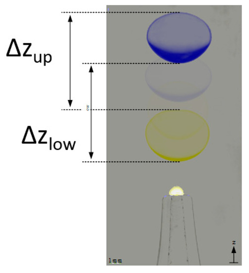
Figure 5.
Illustration of the velocity determination method with a static reference frame on a rising toluene droplet in water.
The velocities are calculated based on the pixel differences (Δzup and Δzlow) between image frames, the frame rates (FPS), the measure of length ML and the difference in between the frames Δnframes. The measurements from the top and bottom are averaged to reduce the influence of droplet deformations in between the frames. In combination with the already known inner nozzle diameter, a measure of length ML for the single pixel in the image can be derived.
The measured values are compared to the calculated ones. The solution of the equation of motion with and without taking into consideration the wall effects is used for comparison.
This is derived from an equilibrium of forces for a rising droplet: the buoyancy force Fb (11), the inertia force Fi,r (12) and the drag force Fd (13)
From the force balance, an expression for the difference in density Δρ can be derived (13) where Vp is the volume of the droplet. For the determination, it is assumed that the droplet is rotationally symmetric, and the projection area of the droplet is equal to the orthogonal area. The volume integral is calculated by a rotation around the x-axis. To determine the volume, a volume integral is used. Therefore, an equation for the contour line of the droplet needs to be determined. This task is solved by an algorithm that uses the labels of the segmentation. It searches for droplets with the assigned label “detached droplet” and determines which labels can be seen in the 4-neighborhood of the analyzed pixel. If one pixel with the label “background” and one pixel with the label “detached droplet” is found in the 4-pixel-neighborhood it is assigned as a pixel of the contour line of the droplet. The positions of the pixels that form the contour line are stored, and afterward, a function consisting of lots of third-order polynomials is fitted through these points. The exact count of subsections depends on the size of the droplet.
As the density of the dispersed phase influences both sides, this equation has to be solved iteratively. The second equation for the difference in density (14) ensures continuity and is used to set up a system of equations which is solved by Newton’s method for multidimensional systems (15). Here k is the iteration step and J is the Jacobian matrix. The function f is a differentiable function with f: ℝ2 → ℝ2 [16]. The problem is set up to find the zeros of the function f by varying the difference in density and the density of the dispersed phase [17].
Additionally, it should be mentioned that the resulting Jacobian matrix for the rising droplet only contains scalar values (17). Therefore, it is not necessary to update the Jacobian matrix in every iteration step; this reduces the complexity and, as a result, the computation time [17].
To ensure the convergence of the procedure, the initial values are chosen, as shown in Table 4. The selection includes that (14) is initially fulfilled, the values are non-negative and that the density of the dispersed phase is smaller than the density of the continuous phase. Moreover, it is considered that the dispersed phase in this work is also a liquid. Accordingly, the densities should be in a similar range.
Table 4.
Initial values for Newton’s method.
For the density calculation with an iterative Newton method, initial values have to be chosen beforehand. For the density difference, a value of 0.25 times the density of the continuous phase is used. The calculation of the dispersed phase density is derived by the Newton method with an initial value of 0.75: the density of the continuous phase. The abort criterion is provided by an error estimate for the difference in density based on two sequential iteration steps (see (18)). As Newton’s method converges fast for reasonable initial conditions, due to local quadratic convergence, the abortion criterion is set to a relatively low value. The chosen criterion ensures that the error contributed by the iteration is minimal [17] and it does not have a noticeable influence on the overall accuracy of the post-processing procedure as this mainly depends on the accuracy of the measured parameters.
Furthermore, the equation of motion for a droplet can be derived from the force balance (10). Together with Equation (19), it leads to an ordinary differential equation for the droplet’s velocity, as shown in Formula (20).
Additionally, an expansion of the force balance by a virtual mass term is possible for small droplets and low Reynolds numbers [18]. The virtual mass force is shown in Equation (21) and takes the acceleration of the surrounding fluid by the moving droplet into account [19].
In this work, the velocity of the surrounding fluid u is in good approximation equal to zero, which simplifies the equation. Moreover, it can be useful to add an acceleration factor α [19] that can be used to increase the quality of the modeled velocity curves for a specific system. The implemented equation for the virtual mass force can be seen in (22).
The resulting differential equation for the droplet’s rising velocity is shown in (23).
The influence of the virtual mass force and the acceleration factor on the velocity curve of a spherical droplet in a tube is illustrated in Figure 6. The curves are the solutions of Equation (23) for a droplet diameter of 4.4 mm and the system n-butyl acetate (dispersed phase)/water (continuous phase) at 20 °C. The drag coefficient was modeled by a correlation that takes the Reynolds number, the droplet shape and wall effects into account (see Equation (20)).
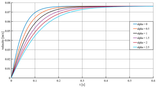
Figure 6.
Velocity curves of a spherical rising droplet with a diameter of 4.4 mm for different values of the acceleration factor α in a tube with a diameter of 15 mm and for the system n-butyl acetate–water.
It can be seen that there is no influence of the virtual mass force and the acceleration factor on the terminal velocity, but the time until it is reached elongates because of a slower acceleration. The curve with α = 0 represents the case without the virtual mass force (20) and reaches the terminal velocity first. The data for Figure 6 can be found in the Data Availability Statement.
The following diagram in Figure 7 includes two correlations for comparison. The first upper boundary (indicated in red) depicts the solution of the equation of motion without the consideration of wall effects. The lower black boundary depicts the correlation including wall effects. However, this correlation was not set up for droplets originally.
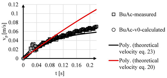
Figure 7.
Velocity of measured (□) and calculated (○) drops. A correlation of the solution of the equation of motion without the consideration of wall effect (red line, Equation (20)) and the correlation of Bäumler et al. [13] including wall effects for comparison (lower black boundary, Equation (23)).
By comparing the calculated data (○) with the two correlations (red and black lines), it becomes apparent that the calculated data points fit the correlation better without wall effects. However, by comparing the actual measured data with the solution of the equation of motion without the consideration of wall effects (black line), it becomes apparent that the data points fit the correlation including wall effects much better even if it is not for droplets but for spheres. Therefore, the use of this drag coefficient correlation (Equation (23)) seems reasonable.
It can be noted that the rising velocity linearly increases over time from 0 m s−1 in the beginning to 0.07 m s−1 after 0.22 s and follows a logarithmic course. Overall, the curve has a lightly periodic shape because the droplets perform an upward motion.
Moreover, a slight jump in the curve occurs between 0.02 and 0.04 s. That is precisely the moment when the droplet detaches. This leads to a sudden stop of detachment force on the cannula and thus an acceleration occurs followed by a velocity decrease as the droplet stabilizes its form.
3.3. Flow Resistance & Drag Coefficient
The flow resistance of a particle is mainly dependent on the combination of two components, the pressure resistance and the friction resistance [1]. The pressure resistance results from the pressure difference between the stagnation point on the front of the droplet and the backside (see Section 2.2). The resulting pressure force (30) only depends on the pressure difference Δp and the orthogonal area Aortho [18]. Accordingly, small orthogonal areas are beneficial to decrease pressure resistance.
The second component of the overall flow resistance is friction, which results from the shearing of the fluid molecules of the surrounding fluid on the surface of the particle. The friction force (31) depends on the shear stress at the surface τs and the surface in contact S. [18]
The overall resistance force (drag) results from the combination of these two components (32). A dimensionless form of this Equation (34) can be derived if it is divided by the dynamic pressure (33) and the orthogonal area [18].
The dimensionless forces can be grasped as resistance coefficients (35), where cd is the overall drag coefficient. The pressure influence is represented by and the friction by .
Depending on the particle’s shape and the surrounding flow, the influence of both components on the overall drag coefficient can rise or fall. In the case of droplets, additional effects such as surface deformation have to be taken into account. [20] Therefore, the modeling of the flow resistance for a rising droplet is significantly more complex, but still very important, as the accurate determination of the drag coefficient plays an important role. It directly influences the calculation of the dispersed phase’s density. The surface deformation of the moving droplet complicates the calculation and the correlations generally fail since a perfect sphere cannot be assumed. [20] Still, there exists a wide variety of different empirical correlations to calculate the drag coefficients for free rising or sinking particles, especially for spheres. Overviews are given by Barati et al. [21] and Kelbaliyev [22]. The correlations often depend on the Reynolds number Re and have a validity range that also depends on the Reynolds number.
Three different correlations for the drag coefficient of a solid sphere (24), a solid ellipsoid (prolate) (37) and a free rising droplet (no wall effects included) (24) depending on the Reynolds number are shown below [22]. Equation (26) was derived by fitting an exponential function on the data from Chang et al. (1992) [23].
A comparison of these three correlations in the range of 80 < Re < 1530 is shown in Figure A1. It can be seen that the curves of the solid sphere and solid prolate have a very similar course even if the absolute values of the drag coefficient are smaller for the prolate. Both start with high values for the drag coefficient at lower Reynolds numbers and end with low values at higher Reynolds numbers. This follows from the flow separation. For increasing Re, the separation point of the flow moves from the backside closer to the front and therefore reduces the friction resistance. The difference in the absolute values of the drag coefficient for the prolate and the sphere results mainly from the smaller cross-sectional area in the direction of the flow in the case of the prolate (smaller pressure resistance, see Figure 8) [24]. The drag coefficients of droplets are even lower than the ones for prolate shapes at a low Re because of the flexible surface [5]. For increasing Re, the drag coefficient rises again. This follows from the deformation of the droplet, which results in an oblate or a cap for a high Re (see Figure 8). Accordingly, the flow resistance rises again as the cross-sectional area is bigger (pressure resistance rises) [24].
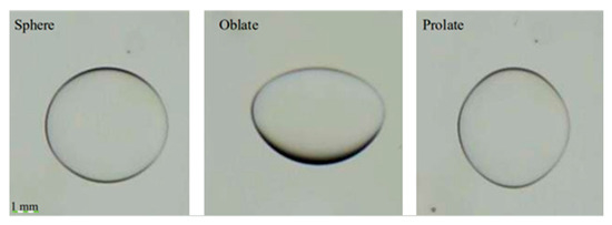
Figure 8.
Shapes of droplets: spherical (left), oblate form (center) and prolate (right). In the oblate shape, the diameter is larger than the height. In the prolate shape, the height is larger than the diameter.
The aspect ratio is calculated by dividing the width of the droplet by the height of the droplet, and thus the projected area of the rising droplet is described. On the other hand, the wall factor describes the influence of the tube wall concerning the flow around the droplet [25].
The drag coefficient is one of the most important parameters since it influences the force balance directly and therefore impacts the calculation of the droplet’s density. To illustrate the influence of the drag coefficient, the shape factor is used, which is based on the aspect ratio shown in Equation (33).
The resulting shape factors are plotted against the aspect ratios (Equation (34) droplet width divided by its height) shown in Figure 9. All investigated liquid systems and nozzles are covered in the graph.
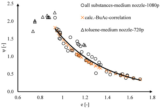
Figure 9.
Plot of the determined shape factors against the aspect ratios of the droplets for different liquid systems and optical resolutions.
The black data points represent the medium nozzle; the resolution of 1080 p is represented by circles and 720 p by triangles. Moreover, the black circles represent a compressed version of all three liquid–liquid systems.
The black triangles are separate from the rest of the data points. This is not surprising, since at lower resolutions the measurement is more susceptible to minor changes and the weighting of a single pixel is higher. For all other measurements there is a trend that with higher aspect ratios, the shape factor decreases exponentially.
The red x markers are values generated by a correlation which only uses n-butyl acetate measurements and is shown in Equation (35) [24].
On the other hand, the black dotted line is also coming from a correlation that only uses measurements with a resolution of 1080 p. The correlation is shown in Equation (36).
It is remarkable that those two graphs are similar; it can be inferred that a transfer to other fluid systems is applicable [25].
3.4. Density
The results for the calculation of the density of the dispersed phase of an n-butyl acetate–water system is shown in Figure 10.
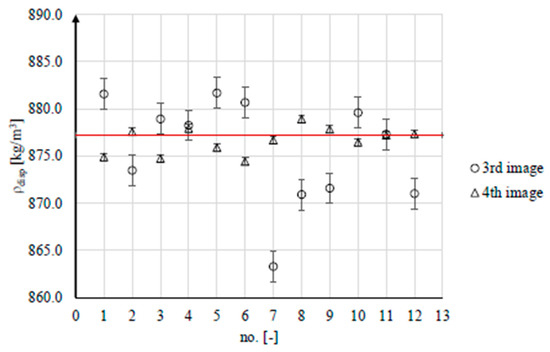
Figure 10.
Results of the density measurement for n-butyl acetate droplets based on the third and fourth images after the reference frame. The horizontal line marks the reference value from the literature [26].
The densities of the third and fourth frames after the reference frame are used to evaluate the densities. The reference frame is the first image which is detected by the search algorithm as a detached droplet. Since droplet formation takes time, the first frame after the reference frame and later frames should be avoided for evaluation because the potential to cause vast deviations is higher.
In the graphic, the red line illustrates the density value from the literature. Most of the points lie in a scope of ±5% around the literature value, where the maximum deviation lies in a range from −1.6% to 0.5%. Moreover, the graphic of the results shows that for the fourth image, the fluctuation around the literature value is much less than for the third image.
The mean, standard deviation and fluctuation margin are shown in Table 5.
Table 5.
Mean value, standard deviation, and fluctuation margin of the density determinations on the system n-butyl acetate–water. The results are based on the third and fourth frames after the reference frame.
The results of the standard deviation prove that the densities captured in the third image after the reference frame scatter stronger than the fourth one. In comparison, online applications such as oscillating/vibration forks for density estimation have uncertainties in a range from ±0.1 kg m−3 to 0.5 kg m−3 [27]. Since the density measurement working with the fourth picture indicates a standard deviation of 1.4 kg m−3, a good starting point for a cheap and quick measurement approach is created. Problems in measurements can be caused by air bubbles.
3.5. Interfacial Tension
The interfacial tension is an effect which takes place at the interface of two immiscible liquids, in the specific case of this work, liquid–liquid systems [28]. It is a result of the attractive and repulsive forces of the two phases.
In general, the interfacial tension can be described as force F per length of the boundary l, or ratio of energy increase ΔE to surface increase ΔS.
In this work, the main focus will be on the formation of static bubbles, or the region for Weber numbers below 2, as it is the basis for the development of the post-processing algorithm and the calculation of the interfacial tension in the investigated liquid–liquid systems. For the physical modeling of static droplet formation, a quasi-stationary force balance (38) between the buoyancy force Fb (39), the viscous force Fη (40), the inertia force Fi (41) and the surface force Fσ (42) is applicable. [20,29]
Figure 11 shows a schematic representation of the droplet formation at the nozzle and the acting forces. The size of the red arrows indicates the influence of the different forces on quasi-stationary droplet formation at low-volume flows.
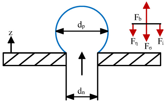
Figure 11.
Equilibrium of forces for static droplet formation at the nozzle. Force balance taken from [29].
The forces depend on various liquid parameters such as the interfacial tension, the viscosity ηc and density ρc of the continuous phase and the density of the dispersed phase ρdisp. Moreover, geometric parameters such as the diameters of the nozzle dn and particles dp are relevant. Finally, the volume flow in the nozzle and gravity g are influential. Since the diameter of the particle is a third-order term, it exhibits the highest influence on the overall force balance.
This equation will be used to calculate the interfacial tension in the post-processing routine. Based on the force balance, an expression for the interfacial tension can be derived (43).
In Figure 12, the third and fourth image after the reference image is used. The thick horizontal line indicates the literature value for the interfacial tension. The measurements of the third image overestimate and the measurements of the fourth image underestimate the marked literature value for the interfacial tension. All of the data points lie in a range from 12.75 mN m−1 to 15.25 mN m−1. The trueness of the investigated system thus is in a range from −1 to +0.4 mN m−1 with a precision of ±0.3 to ±0.6 mN m−1.
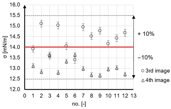
Figure 12.
Results of the determination of the interfacial tension of n-butyl acetate droplets in water by using the third and fourth frames after the first frame of the droplet’s detachment. The thick horizontal line is taken as reference from literature [26].
4. Conclusions and Future Work
Fluid properties are laborious to determine, in particular for liquid mixtures with different compositions. In this work, a quick and simple AI-based approach for the online measurement of liquid parameters was developed. The target figures were the density and interfacial tension of rising droplets. For this, a neural network was successfully trained to recognize and segment droplets of three liquid systems; it was highly accurate, as the network reached scores of over 97.7% for all relevant segmentation parameters. By comparing the training settings and training results with networks presented in the literature, a basic guideline for segmenting droplets with the assistance of an AI algorithm has been derived.
Based on all this, a complex post-processing routine was developed that generates a big variety of geometric and physical data pertaining to the investigated droplets. Hence, this routine can also be used to investigate rising droplets as a research tool and is able to calculate even more parameters as dimensionless numbers based on the measured data. Accuracy describes the proximity of a measurement or prediction to the true value, while precision refers to the degree of scatter or variability in a set of measurements or predictions. The accuracy of the method for the determination of densities is approx. ±1 kg m−3 with a precision of approx. ±11 kg m−3. The accuracy of the determination of the interfacial tension is approx. ±1.25 mN m−1 and the precision is approx. ±0.6 mN m−1. Therefore, precision is the main target for further enhancement.
A major limitation is that the uprising fluid needs to have a lighter density than water. An envisaged future improvement is a rotated setup with the heavier liquid fed from the top to broaden the applicability spectrum of this method in the near future. Fluid mixtures are the major aim to investigate with an automated setup, where temperature and mixture concentration can be varied in a wide range. Rising gas bubbles will be tested in different liquid environments as well. With the inverted setup, falling droplets can be automatically investigated concerning properties such as density, surface tension and viscosity. This will lead to the rapid automated generation of large data sets for interesting liquid mixtures in research and development.
Author Contributions
Conceptualization, N.K., L.N., P.M. and K.L.; methodology, L.N. and P.M.; software, L.N. and P.M.; validation, L.N., P.M. and K.L.; formal analysis, L.N., P.M. and K.L.; investigation, L.N., P.M. and K.L.; resources, L.N., P.M., K.L. and N.K.; data curation, L.N., P.M. and K.L.; writing—original draft preparation, L.N.; writing—review and editing, L.N., P.M., K.L. and N.K.; visualization, L.N., P.M.; supervision, L.N. and N.K.; project administration, N.K.; funding acquisition, N.K. All authors have read and agreed to the published version of the manuscript.
Funding
This research was funded by the BMWK (German Federal Ministry of Economic Affairs and Climate Action, grant number 01MK20014S).
Data Availability Statement
Data available in a publicly accessible repository that does not issue DOIs. This data can be found here: [https://tu-dortmund.sciebo.de/s/YS8QlCbSO1zUFCB] (accessed on 31 March 2023).
Acknowledgments
The authors want to thank Carsten Schrömges for his lab assistance. The authors want to thank Julia Schuler for performing accurate measurements of the cannula diameters using the micro CT.
Conflicts of Interest
The authors declare no conflict of interest. The funders had no role in the design of the study; in the collection, analyses, or interpretation of data; in the writing of the manuscript; or in the decision to publish the results.
Abbreviations
| Latin Symbols | ||
| A | cross-sectional area | - |
| b | threshold | - |
| cd | drag coefficient | - |
| dp | droplet diameter | m |
| E | energy | Nm |
| F | force | N |
| g | gravitation acceleration | m s−2 |
| J | Jacobian matrix | - |
| S | surface | m 2 |
| t | time | s |
| Vint | internal volume | mL |
| v | velocity | - |
| w | weight function of a neural network | - |
| x | input into a neural network | - |
| z | transfer function | - |
| Greek Symbols | ||
| α | factor | - |
| η | dynamic viscosity | kg m−2 s−3 |
| Ψ | correlation function | - |
| ρ | density | kg m−3 |
| σ | surface tension | N m−1 |
| τ | shear stress | N m−2 |
| Dimensionless Numbers | ||
| Mo | Morton number | - |
| Re | Reynolds number | - |
| We | Weber number | - |
Appendix A
Appendix A.1
- a.
- Load trained neural network, set image resolution and cannula size and calibrate length per pixel
- b.
- Set filter for minimal pixel for droplet detection
- c.
- Read and then disassemble video
- d.
- Perform image segmentation using trained CNN
- a.
- Detect first image frame with a pixel with the label “detached droplet.” Save the following three images and the image before this frame
- b.
- Determination of area and diameter
- i.
- Filter out areas smaller than set filter area, overwrite falsely detected pixel labels with their most likely neighborhood values
- c.
- Determination of volume from area splines
- i.
- If one pixel with the label neighborhood is assigned as a pixel of the contour line of the droplet
- ii.
- The positions of the pixels that form the contour line are stored and a function (lots of third-order polynomial “splines” are fitted to smaller subsections of the contour, exact count of subsections depends on size of the droplet) is fitted through these points.
- e.
- Calculation of aspect ratio
- a.
- Aspect ratio = diameter width/diameter height of selected images
- f.
- Determination of velocity based on the pixels uprising from image to image and the image’s time difference
- g.
- Show & save segmentation result
Table A1.
Parameters for the velocity curves shown in Section 3.2.
Table A1.
Parameters for the velocity curves shown in Section 3.2.
| Parameter | Value | Unit |
|---|---|---|
| ρc | 997 | kg∙m−3 |
| ρdisp | 877.2 | kg∙m−3 |
| dp | 4.4 | mm |
| dtube | 15 | mm |
| vp (t = 0) | 10−6 | m∙s−1 |
| g | 9.81 | m∙s−2 |
| cd,wall | calculated with (30) | - |

Figure A1.
Correlations for the dependency of the drag coefficient cd on the Reynolds number Re for different shapes and particles [22,23].
Figure A1.
Correlations for the dependency of the drag coefficient cd on the Reynolds number Re for different shapes and particles [22,23].

Table A2.
Resulting trueness and precision for the chemical systems. All data can be found in the link titled “Data availability statement”.
Table A2.
Resulting trueness and precision for the chemical systems. All data can be found in the link titled “Data availability statement”.
| Parameter | n-Butyl Acetate | n-Butanol | Toluene |
|---|---|---|---|
| Trueness | −1 to +0.4 mN m−1 | +0.8 mN m−1 | −1.2 mN m−1 |
| Precision | ±0.3 to ± 0.6 mN m−1 | ±0.2 mN m−1 | ±4.9 mN m−1 |
References
- Kockmann, N.; Bittorf, L.; Krieger, W.; Reichmann, F.; Schmalenberg, M.; Soboll, S. Smart Equipment—A Perspective Paper. Chem. Ing. Tech. 2018, 90, 1806–1822. [Google Scholar] [CrossRef]
- Goodfellow, I.; Bengio, Y.; Courville, A. Deep Learning; Adaptive Computation and Machine Learning Series; MIT Press Ltd.: Cambridge, MA, USA, 2017. [Google Scholar]
- Villalba-Diez, J.; Schmidt, D.; Gevers, R.; Ordieres-Meré, J.; Buchwitz, M.; Wellbrock, W. Deep Learning for Industrial Computer Vision Quality Control in the Printing Industry 4.0. Sensors 2019, 19, 3987. [Google Scholar] [CrossRef] [PubMed]
- Schuler, J.; Neuendorf, L.; Petersen, K.; Kockmann, N. Micro-computed tomography for the 3D time‐resolved investigation of monodisperse droplet generation in a co-flow setup. AIChE J. 2020, 67, e17111. [Google Scholar] [CrossRef]
- Kockmann, N. Digital methods and tools for chemical equipment and plants. React. Chem. Eng. 2019, 4, 1522–1529. [Google Scholar] [CrossRef]
- Ahmad, A.; Song, C.; Tan, R.; Gartler, M.; Klopper, B. Active Learning Application for Recognizing Steps in Chemical Batch Production. In Proceedings of the 2022 IEEE 27th International Conference on Emerging Technologies and Factory Automation (ETFA), Stuttgart, Germany, 6–9 September 2022; IEEE: Stuttgart, Germany, 2022. [Google Scholar]
- Neuendorf, L.M.; Baygi, F.; Kolloch, P.; Kockmann, N. Implementation of a control strategy for hydrodynamics of a stirred liquid–liquid extraction column based on convolutional neural networks. ACS Eng. Au 2022, 2, 369–377. [Google Scholar] [CrossRef]
- Nandakumar, S.C.; Harper, S.; Mitchell, D.; Blanche, J.; Lim, T.; Yamamoto, I.; Flynn, D. Bio-Inspired Multi-Robot Autonomy. arXiv 2022, arXiv:2203.07718. [Google Scholar]
- Wiederkehr, P.; Finkeldey, F.; Merhofe, T. Augmented semantic segmentation for the digitization of grinding tools based on deep learning. CIRP Ann. 2021, 70, 297–300. [Google Scholar] [CrossRef]
- Roshani, G.H.; Ali, P.; Mohammed, S.; Hanus, R.; Abdulkareem, L.; Alanezi, A.; Sattari, M.; Amiri, S.; Nazemi, E.; Eftekhari-Zadeh, E.; et al. Simulation study of utilizing X-ray tube in monitoring systems of liquid petroleum products. Processes 2021, 9, 828. [Google Scholar] [CrossRef]
- Abuqaddom, I.; Mahafzah, B.; Faris, H. Oriented stochastic loss descent algorithm to train very deep multi-layer neural networks without vanishing gradients. Knowl. Based Syst. 2021, 230, 107391. [Google Scholar] [CrossRef]
- Chen, T.-C.; Alizadeh, S.; Alanazi, A.; Guerrero, J.G.; Abo-Dief, H.; Eftekhari-Zadeh, E.; Fouladinia, F. Using ANN and Combined Capacitive Sensors to Predict the Void Fraction for a Two-Phase Homogeneous Fluid Independent of the Liquid Phase Type. Processes 2023, 11, 940. [Google Scholar] [CrossRef]
- Medl, M.; Rajamanickam, V.; Striedner, G.; Newton, J. Development and Validation of an Artificial Neural-Network-Based Optical Density Soft Sensor for a High-Throughput Fermenta-tion System. Processes 2023, 11, 297. [Google Scholar] [CrossRef]
- Clift, R.; Grace, J.; Weber, M. Bubbles, Drops, and Particles; Acad. Press: New York, NY, USA, 1978. [Google Scholar]
- Nielsen, M. (Ed.) Neural Networks and Deep Learning; Determination Press: San Francisco, CA, USA, 2015. [Google Scholar]
- Böckh, P.; Saumweber, C. Fluidmechanik: Einführendes Lehrbuch, 3rd ed.; Springer: Berlin/Heidelberg, Germany, 2013. [Google Scholar]
- Dahmen, W.; Reusken, A. Numerik für Ingenieure und Naturwissenschaftler; Springer-Lehrbuch, Springer: Berlin/Heidelberg, Germany, 2008. [Google Scholar]
- Crowe, C.T. Multiphase Flows with Droplets and Particles, 2nd ed.; CRC Press: Boca Raton, FL, USA, 2012. [Google Scholar]
- Wegener, M.; Grünig, J.; Stüber, J.; Paschedag, A.; Kraume, M. Transient rise velocity and mass transfer of a single drop with interfacial instabilities—Experimental investigations. Chem. Eng. Sci. 2007, 62, 2967–2978. [Google Scholar] [CrossRef]
- Räbiger, N.; Schlüter, M. VDI-Wärmeatlas, 11th ed.; L4 Blasen und Tropfen in technischen Apparaten; Springer Reference; Springer Vieweg: Berlin, Germany, 2013. [Google Scholar]
- Barati, R.; Neyshabouri, S.; Ahmadi, G. Development of empirical models with high accuracy for estimation of drag coefficient of flow around a smooth sphere: An evolutionary approach. Powder Technol. 2014, 257, 11–19. [Google Scholar] [CrossRef]
- Kelbaliyev, G.I. Drag coefficients of variously shaped solid particles, drops, and bubbles. Theor. Found Chem. Eng. 2011, 45, 248–266. [Google Scholar] [CrossRef]
- Chang, C.-C.; Liou, B.-H.; Chern, R. An analytical and numerical study of axisymmetric flow around spheroids. J. Fluid Mech. 1992, 234, 219–246. [Google Scholar] [CrossRef]
- Bohl, W.; Elmendorf, W. Technische Strömungslehre: Stoffeigenschaften von Flüssigkeiten und Gasen, Hydrostatik, Aerostatik, Inkompressible Strömungen, Kompressible Strömungen, Strömungsmesstechnik, 15th ed.; Kamprath-Reihe, Vogel: Würzburg, Germany, 2014. [Google Scholar]
- Kishore, N.; Gu, S. Wall Effects on Flow and Drag Phenomena of Spheroid Particles at Moderate Reynolds Numbers. Ind. Eng. Chem. Res. 2010, 49, 9486–9495. [Google Scholar] [CrossRef]
- Bäumler, K.; Wegener, M.; Paschedag, A.; Bänsch, E. Drop rise velocities and fluid dynamic behavior in standard test systems for liquid/liquid extraction—Experimental and numerical investigations. Chem. Eng. Sci. 2011, 66, 426–439. [Google Scholar] [CrossRef]
- Hradetzky, G.; Sommer, K. Flüssigkeits-Dichtemessung: Übersichtsartikel. Available online: https://physchem.hs-merseburg.de/Dichte.pdf (accessed on 17 March 2021).
- Zierep, J.; Bühler, K. Grundzüge der Strömungslehre: Grundlagen, Statik und Dynamik der Fluide, 9th ed.; Springer Fachmedien: Wiesbaden, Germany, 2013. [Google Scholar]
- Voit, H.; Zeppenfeld, R.; Mersmann, A. Calculation of primary bubble volume in gravitational and centrifugal fields. Chem. Eng. Technol. 1987, 10, 99–103. [Google Scholar] [CrossRef]


Disclaimer/Publisher’s Note: The statements, opinions and data contained in all publications are solely those of the individual author(s) and contributor(s) and not of MDPI and/or the editor(s). MDPI and/or the editor(s) disclaim responsibility for any injury to people or property resulting from any ideas, methods, instructions or products referred to in the content. |
© 2023 by the authors. Licensee MDPI, Basel, Switzerland. This article is an open access article distributed under the terms and conditions of the Creative Commons Attribution (CC BY) license (https://creativecommons.org/licenses/by/4.0/).