Graphic Template Establishment and Productivity Evaluation Model of Post-Fracturing Based on the Fluctuation Pattern of G-Function Curve

Abstract

In the process of fracturing construction in shale gas reservoirs, microseism is a common means and effective method to evaluate the fracturing effect, but it is not suitable for large-scale and large batches due to its high applicability conditions and cost. Therefore, a concise, fast and low-cost post-fracturing effect evaluation method is needed to evaluate the complexity of fractures formed by fracturing in shale gas reservoirs. In this paper, based on the basic theory of the G-function, the free variable μ was introduced to correct the filter loss coefficient with the participation of natural fractures, and thousands of G-function curves were plotted with fracturing data from hundreds of gas wells in the southern Fuling shale gas field in China. Through the feature analysis of the curve morphology, a G-function graphic template conforming to the block was established, which contains four types and eight morphologies. Four characteristic parameters in the G-function curve were selected to establish a productivity evaluation model for shale gas wells. Based on the validation results, it can be seen that the G-function graphic template and productivity evaluation model proposed by the author had a good correlation with the post-fracturing productivity of shale gas wells, which provided a fast, economical and accurate method for the post-fracturing effect evaluation and productivity evaluation of shale gas wells and can effectively provide feedback on the field fracturing effect and guide subsequent fracturing construction.

1. Introduction

With the development of unconventional natural gas, the exploration field of oil and gas resources is becoming more and more extensive, and the difficulty of extraction is also increasing [1]. The development of shale gas, one of the most prominent commercially exploitable unconventional natural gases, has attracted much attention at home and abroad, and has now become a strategic energy source for China [2]. Since shale gas reservoirs have typical ultra-low permeability and low porosity and their matrix pore diameters are only between a few and several hundred nanometers, a certain scale of hydraulic fracturing is required for the development process. Hydraulic fracturing can create large-scale artificial fractures in shale reservoirs [3,4] and the fracturing effect determines the production of shale gas wells. Microseismic monitoring technology is an effective means to evaluate its effect [5,6,7,8]. However, due to the high cost and operational difficulties of microseismic monitoring technology, not every well in shale gas well development has been microseismically monitored, and therefore it cannot be used as a conventional monitoring tool to evaluate the fracturing effect of each section.

The post-fracturing productivity evaluation of shale gas is a particularly important part of shale gas development. At present, there are many post-fracturing evaluation techniques, but they are single and complex. Most post-fracturing productivity evaluation methods are based on production mechanisms or machine learning methods for prediction, and traditional methods are not able to accurately predict the post-fracturing productivity [9]. In 2007, M. K. Rahman et al. [10] proposed a production analysis model for gas reservoirs after hydraulic fracturing to achieve detailed production predictions. In 2012, Rahman M. M. and Rahman M. K. [11] optimized sand emergence during fracturing by modeling the critical pressure drop of predicted gas wells. In the process of unconventional gas exploration and development, conventional post-fracturing evaluation techniques cannot accurately describe the true post-fracturing state of the formation due to the increasingly complex reservoir environment, and they are limited [12]. The reason for this is that the shale gas production process is influenced by many factors such as geology and engineering, with strong non-linear characteristics, and both the production mechanism and machine term are based on basic data to do research, which do not truly reflect the post-frac condition of the formation. Therefore, by analyzing the pressure drop process after stopping the pump through the fracturing second point data at the construction site, the complexity of the fracture morphology formed in the formation after fracturing can be evaluated, which can more accurately reflect the real situation in the formation, and then obtain the fracture morphology and productivity evaluation of shale gas horizontal wells after multi-stage fracturing.

The pressure drop analysis method was proposed by Nolte [13,14] in 1979 and has been continuously improved by scholars in related fields. In 1996, Mukherjee and Barree [15] first proposed to apply the G-function to a small-scale fracturing test to analyze the filtration mechanism of the fracturing fluid and judge the filtration type according to the curve shape of the superposition derivative of the G-function. They proposed four fracture characteristics to correspond to the curve shape, which were the continuous expansion of the fracture after the pump is stopped, the pressure-independent filtration, the pressure-controlled filtration and the filtration of the fracture height. In 2000, the G-function formulation was modified by R. Henry Jacot and Bruce R. Meyer [16] and the natural development factor β was proposed to quantitatively characterize the communication between natural fractures and induced fractures. In subsequent studies, different scholars [17,18,19,20,21,22,23,24,25] have successively developed G-function plates applicable to volcanic reservoirs based on construction curve pressure drop analyses and used G-function fluctuation characteristics to evaluate the complexity of the fractures. In 2022, Xiao Yang [26] analyzed the fracture morphology of the reservoir based on G-functions using pressure drop data after the fracture pump stoppage, which was subsequently verified using microseismic data.

However, in the process of oil and gas field development, the main purpose is to improve the production and recovery rate of oil and gas wells and any other related research is to provide a basis for the production capacity and recovery rate. The G-function theory, although much research has been done in the fracture evaluation, is not directly related to the production capacity, and this approach has major drawbacks in that it assumes conditions different from the actual fracturing site, such as assuming a fixed fracture height, ignoring the initial filtration loss and the change in the fracture morphology after pump stoppage are ignored, and the filtration loss coefficient is independent of pressure. Therefore, the establishment of a shale post-fracturing fracture evaluation plate and capacity evaluation model based on a G-function curve fluctuation analysis is much needed for the current shale gas field development. This paper analyzes the pressure drop process after pump stoppage by using the fracturing construction data from the construction site to evaluate the complexity of the fracture pattern formed in the formation after fracturing, which can more accurately reflect the real situation in the formation. We then propose capacity evaluation indicators and models based on the curve patterns to obtain the fracture patterns and capacity evaluation of shale gas horizontal wells after multi-stage fracturing to guide the fracturing construction.

2. Materials and Methods

The G-function is based on the principle of mass conservation in the pumping procedure, i.e., pumped fluid volume−initial filtration volume = fracture volume. i.e., we have:

$${{\displaystyle \int }}_0^{t}q(t)dt-V_l(t)-V_{sp}(t)=V_{f(t)}$$

(1)

Eq:

$$V_l(t)=2{{\displaystyle \int }}_0^t{{\displaystyle \int }}_0^A\frac{c(A,t)}{{(t-\tau (A))}^{{\alpha }_{\tau }}}dAdt$$

(2)

$$v_{sp}(t)=2S_{p}A(t)$$

$$A(t)=H_{P}L(t)$$

$\tau (A)=t{\left(\frac{A}{A(t)}\right)}^{\frac{1}{a_{\tau }}}$ (${\alpha }_{\tau }=\frac{1}{2}$, According to the square root filter loss model proposed by Carter [27]).

Where: $q(t)$ is the pumping displacement, $m^3/\min$; $V_l(t)$ is the volume of fracturing fluid filtration loss between pumping, $m^3$; $V_{sp}(t)$ is the initial filtration loss coefficient, $m^3/m^2$; $H_P$ is the fracture filtration loss height, m; $A(t)$ is the fracture filtration loss area on one side, $m^2$; $L(t)$ is the fracture length formed, m.

After stopping the pump, the filtration loss volume of the fracturing fluid is obtained from Equation (2):

$$\mathsf{\Delta }{V}_l(t)=2{{\displaystyle \int }}_{t_p}^t{{\displaystyle \int }}_0^A\frac{c(A,t)}{{(t-\tau (A))}^{{\alpha }_{\tau }}}dAdt$$

(3)

Assuming that the filter loss coefficient is a function of time, the differentiation of t in Equation (3) yields:

$$\frac{d\mathsf{\Delta }{V}_l(t)}{dt}=2C(t){{\displaystyle \int }}_0^A\frac{1}{{(t-\tau (A))}^{a_{\tau }}}dA=\frac{\pi }{2}C(t)A\left(t_p\right)\sqrt{t_p}\frac{d}{dt}G\left({\alpha }_a,0,\theta \right)$$

(4)

According to the expression of the G-function established by the classical Nolte theory, G in Equation (4) is:

$$G\left({\alpha }_a,0,\theta \right)=\frac{4}{\pi }{{\displaystyle \int }}_1^{\theta }{\xi }^{{\alpha }_a+{\alpha }_{c2}-1/2}{{\displaystyle \int }}_0^{\xi -{\alpha }_a}\frac{1}{{\left(1-{\lambda }^{1/{\alpha }_a}\right)}^{1/2}}d\lambda d\xi$$

(5)

$$\theta =\frac{t}{t_p}$$

(6)

where, θ is the dimensionless time; ${\alpha }_a$ is the parameter of the filter loss area with time; ${\alpha }_c$ is the parameter of the filter loss coefficient with time; $t_p$ is the pumping time, min. Since the square root filter loss is assumed, ${\alpha }_{\tau }$ is taken as 0.5; $C(t)$ in Equation (4) is not within the product function and ${\alpha }_{c2}$ is taken as 0 here.

Since the change in the filtering loss coefficient will be reflected in the shape of the G-function curve, the G-function is divided into two categories as follows:

(1) When the filter loss coefficient is not correlated with the pressure, the pressure drop equation can be expressed as:

$$\frac{dP}{ dG}=\Delta P_{\mathrm{f}}\left(t_{\mathrm{p}}\right)\frac{1-{\eta }_{\mathrm{s}}}{2{\eta }_{\mathrm{s}}\mathsf{\Phi }}\frac{C(t)}{C\left(t_{\mathrm{p}}\right)}$$

(7)

Let $P=ISIP-P(t)$, in the formula.

Where ${\eta }_{\mathrm{s}}$ is the fracture fluid efficiency at the end of pumping (i.e., b) after the initial filtration loss; $\mathsf{\Delta }{P}_{\mathrm{f}}\left(t_{\mathrm{p}}\right)$ is the net in-fracture pressure at the end of pumping, MPa; ISIP is the instantaneous shut-in pressure, MPa, and it is the fracture fluid filtration loss parameter at the beginning of fracture extension. In this paper, the superimposed derivative $G\frac{dP}{ dG}$ of the G-function was used to evaluate the post-pumping fracture and production capacity by multiplying the left and right sides of Equation (7) by one G, i.e., we can obtain:

$$G\frac{dP}{dG}=\Delta P_{\mathrm{f}}\left(t_{\mathrm{p}}\right)\frac{1-{\eta }_s}{2{\eta }_s\Phi }\frac{C(t)}{C\left(t_{\mathrm{p}}\right)}G\left({\alpha }_a,0,\theta \right)$$

(8)

At this time, the filtration loss coefficient is only limited by the filter cake or reservoir and is constant, the G-function superposition inverse and G-function causeless time are linear, the filtration loss coefficient only changes when the fracture is closed and the fracture that meets this characteristic can be regarded as a conventional bifurcation.

(2) When the natural fractures in the formation open during on-site fracturing, it will cause changes in the filtration loss coefficient, which is pressure-dependent at this time. Specifically, the natural fractures originally existing in the formation will converge with the induced fractures generated during hydraulic fracturing construction. Due to the formation of the original formation energy deficiency, it is no longer a single fracture cross seam, and the filtration loss rate of the fracturing fluid in the fracture network increases sharply due to the addition of natural fractures, which leads to the change in the filtration loss coefficient.

Therefore, when the fracture pressure is higher than the closure pressure of the natural fracture, the filtration loss of the fracturing fluid occurs not only in the induced fracture but also in the natural fracture that has been communicated, and the filtration loss factor is defined as C_L1. In the process of gradual pressure reduction in the fracture afterwards, the filtration loss of the fracturing fluid exists only in the main fracture due to the gradual closure of the natural fracture, and the filtration loss coefficient at this time is defined as C_L2. Foreign scholars Mayer and Jacot [16] proposed the equation for the filtration loss coefficient of this process expressed as:

$$C_L\left[P\left(t\right)\right]=\left\{\begin{array}{l}{C}_{L1},P(t)\ge P_{f_0}\\ C_{L2},P(t)<P_{f_0}\end{array}\right.$$

(9)

where, P_f0 is the pressure threshold when the natural fracture is closed (opened).

Obviously, the filter loss coefficient in the above equation is a sudden change model [28], but in the actual fracturing process, the natural fracture closure is dynamic and does not happen overnight. Therefore, we must introduce a free variable μ in characterizing the variation process of the filter loss coefficient during the natural fracture closure based on Equation (9).

$$C_L[P(t)]=\left\{\begin{array}{l}{C}_{L1},P(t)>P_{f0}\\ (C_{L1}-C_{L2})\frac{\exp \left[\mu \frac{P(t)}{P_{f0}}\right]-\exp \left(\mu \frac{P_{ci}}{P_{f0}}\right)}{\exp (\mu )-\exp \left(\mu \frac{P_{ci}}{P_{f0}}\right)}+C_{L2},P_{f0}\ge P(t)\\ C_{L2},P_{ci}>P(t)>P_c\end{array}\right.\ge P_{ci}$$

(10)

where P_c is the final closure pressure of all fractures and P_ci is the formation pressure after all natural fractures are closed (only induced fractures are involved in the filtration).

It can be seen from Formula (10) that due to the introduction of free variables, the filtration coefficient also changes with the change in μ, so the superposition derivative of the G-function derivative will also change with the change in the filtration coefficient. Starting from the characteristics of different curve shapes, the fracture shapes corresponding to each curve shape are summarized, which can effectively help the efficient fracturing construction of shale gas wells. The following will analyze and summarize the massive actual fracturing data from the southern region of Fuling, China and establish a G-function chart that conforms to the characteristics of the block.

3. Plate and Model Building

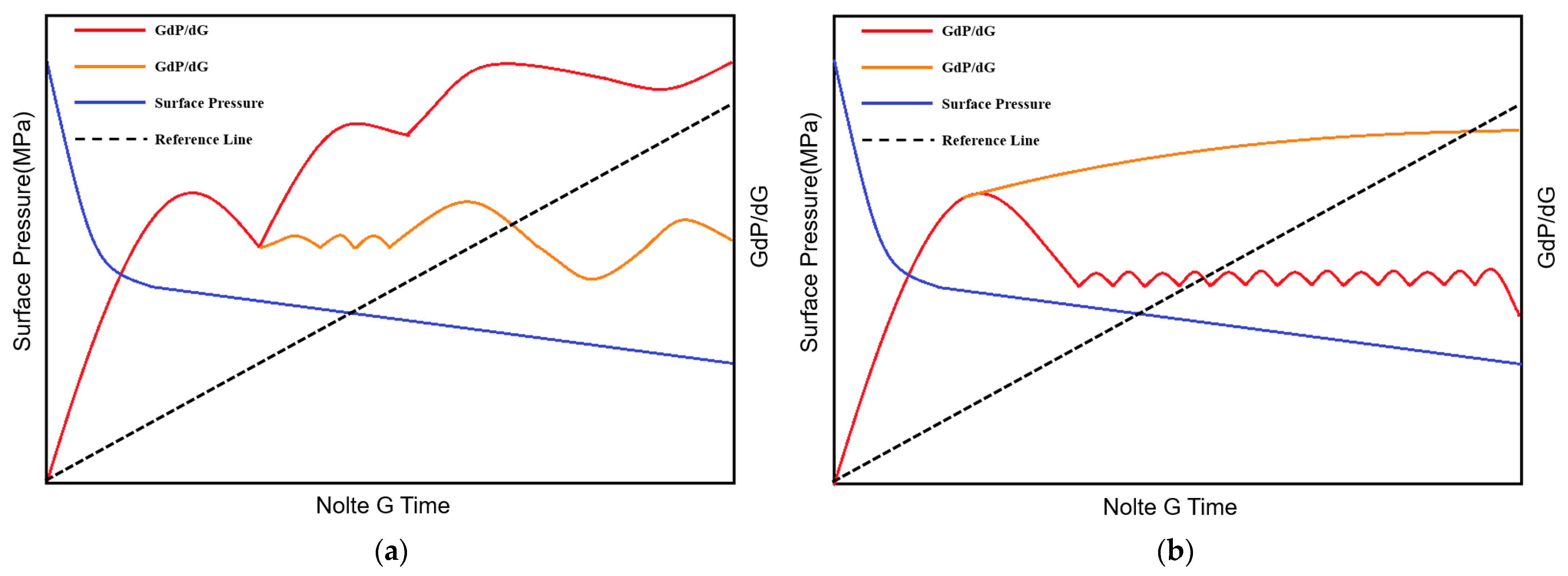
3.1. Establishment of the G-Functional Graphic Template

Based on the above analysis of the filtration loss coefficient, the author conducted thousands of G-function curves from the fracturing data of hundreds of shale gas wells and screened them. The G-function images of wells with a high initial production and high cumulative production were selected separately, from which the G-function characteristics of different types of high-producing wells were identified, categorized and analyzed. The high-producing section was selected from wells with production profile data, analyzed for the G-function characteristics of the section and matched to G-function images of the high-producing wells. This was followed by a comparative analysis in relation to the production as well as microseismic data, and a plate containing eight G-function morphology models in four categories was developed. The details are shown in Figure 1 and Figure 2.

We carried out the matching of the corresponding crack morphology according to the proposed G-function version and the results are shown in Figure 2.

The main morphological categories of the G-function chart:

Type I G-function: The G-function superimposed derivative $G\frac{dP}{dG}$ starts to rise rapidly, generally greater than or equal to 2. At the beginning of the curve, the area of upward convexity is large and then the curve continues to rise with fluctuations or tends to be stable with a large number of fluctuations. This is due to the good fracturing effect of the main seam, and the fluid is quickly lost in the main seam after the pump is stopped, so the initial slope of the curve is large and then the fluid is lost in the branch seam and the natural fracture. As the branch fractures and natural fractures close continuously, the curve is accompanied by a lot of fluctuations, until after the branch fractures and natural fractures close, the fluid is only lost in the main fractures and the curve pattern starts to level off. This type of G-function represents that the section is well fractured by the main fractures and well developed by the branch fractures, which communicate with the natural fractures and form a complex fracture network (Main fractures + Branch fractures + Natural fractures).

Type II G-function: This type of G-function curve is characterized by a rapid rise in $G\frac{dP}{dG}$ after well shutdown, with the end generally greater than or equal to 2 and the area of the convex part of the curve is large. Thereafter the curve continues to rise slowly or falls back rapidly and then tends to be stable, with no fluctuation or accompanied by a small fluctuation during the period, representing a good fracturing effect of the main fracture and a well-developed branch fracture, which communicates with a few natural fractures and forms a complex fracture network (Main fractures + Branch fractures + few Natural fractures).

Type III G-function: The curve pattern of this type of G-function is characterized by a slow rise in the overall trend after pump stoppage, with the end generally less than or equal to 2. The rise in the curve is accompanied by a large number of fluctuations (the fluctuation trend can be large or small), which corresponds to a slow rate of fluid filtration in the fracture. This type of curve means that the fracturing effect of the main fracture is average, the branch fracture is not well developed and the fracturing construction has communicated some natural fractures and formed a small-scale fracture network (Main fracture + Natural fracture).

Type IV G-function: This type of G-function curve form is characterized by a steady rise in a linear-like form from the time of pump stop, with no or little fluctuation during the period. Corresponding to the poor fracturing effect of the main fractures, the branch fractures are not developed, not communicating with natural fractures and mainly exist in the form of a single fracture (Main Fracture).

Based on the above summarized four types of shale gas well post-fracturing capacity evaluation plates, it helps the fracturing construction site to quickly categorize and diagnose the G-function curves drawn after fracturing. In turn, it can evaluate and guide the subsequent fracturing, and promote the shale gas well segmentation fracturing post-fracturing real-time analysis means to maturity.

3.2. G-Function Yield Evaluation Model

By comparing and analyzing the G-function curve shape drawn by massive actual fracturing construction data, the indicators that can represent the curve shape were extracted and the quantitative G-function evaluation index standard was formulated. The evaluation indexes included the average pressure drop velocity V_ΔPt of the inflection point at the first peak of the superposition derivative of the G-function, the slope k of the inflection point at the first peak of the superposition derivative of the G-function, the fluctuation number D of the G-function and the area S below the G-function.

The initial slope k of the superposition derivative of the pressure drop velocity V_ΔPt and G-function was classified as the A₁ index to evaluate the flow of fluid in the main fracture. The wave number D of the G-function and the area S below the derivative curve of the G-function superposition were classified as A₂ indexes to evaluate the flow of fluid in branch fractures (natural fractures). The evaluation index Y of the G-function image was obtained by calculating the evaluation index extracted by an image recognition algorithm by formulating the evaluation standard formula.

$$Y=A_1\times 0.7+A_2\times 0.3$$

(11)

Among them:

  

$A_1=V_1\times 0.3+k\times 0.7$

  

$A_2=D\times 0.5+S\times 0.5$

  

$V_{P_t}=\Delta P/\Delta Nolte G$

  

$k=\Delta G\frac{dP}{dG}/\Delta Nolte G$

S is the area under the $G\frac{dp}{dG}$ curve and D is the number of fluctuations, the curve fluctuations in the right vertical coordinate fluctuation amplitude ≥0.1 is recorded as 1 time.

The above four evaluation indexes could be extracted and calculated based on image recognition, and the reference score of the scoring interval of the G-function curve evaluation index was formulated according to the above formula (

Table 1. The evaluation index of the G-function curve is divided into partitions.

Evaluating Indicator	Interval Score
	0	0.25	0.5	0.75	1
k	<15	15 ≤ k < 30	30 ≤ k < 45	45 ≤ k < 60	≥60
VΔPt	<10	10 ≤ VΔPt < 20	20 ≤ VΔPt < 30	30 ≤ VΔPt < 40	≥40
D	<4	4 ≤ D < 6	6 ≤ D < 8	8 ≤ D < 10	≥10
S	<0.2	0.2 ≤ S < 0.3	0.3 ≤ S < 0.4	0.4 ≤ S < 0.5	≥0.5

), and the parameters of the single section G-function were extracted and scored. The higher the score, the higher the corresponding single section production. A standard line of 0.5 was established to distinguish the high and low production sections, i.e., when the productivity evaluation value Y > 0.5, the section was considered to have a better fracturing effect and higher post-fracturing productivity, and similarly, when Y < 0.5, the section was considered to have a poor fracturing effect and lower productivity.

In the process of data extraction, we needed to perform image grayscale and binarization pre-processing on the curve area. After that, we performed edge detection on the image by a Canny operator, and then detected the number of lines in the region by the Hoffman transform, and then extracted the angle and identified the area under the curve for the lines in the region. The specific operation steps are shown in Figure 3 and part of the image recognition process is shown in Figure 4.

4. Discussion

In order to verify the accuracy of the G-function graphic template, we screened and counted 24 shale gas wells with the production data in three blocks of the shale gas field in southern Fuling, China, and counted the production status as well as the fracturing data and rock mechanics characteristics of each well separately. The G-function curves of the whole section of the well with high initial production (≥18 × 10⁴ m³/d) and low initial production (≤10 × 10⁴ m³/d) were verified graphically. Furthermore, the G-function curves of the high and low production sections of wells with production profile data were validated.

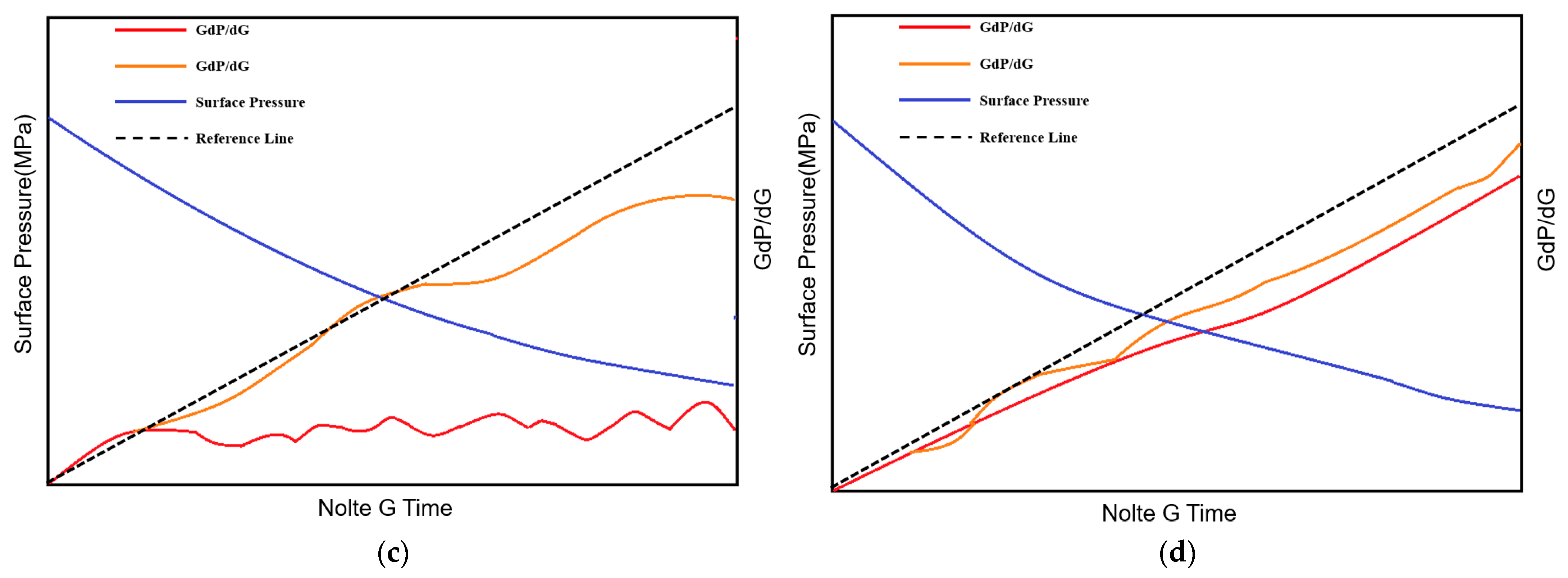
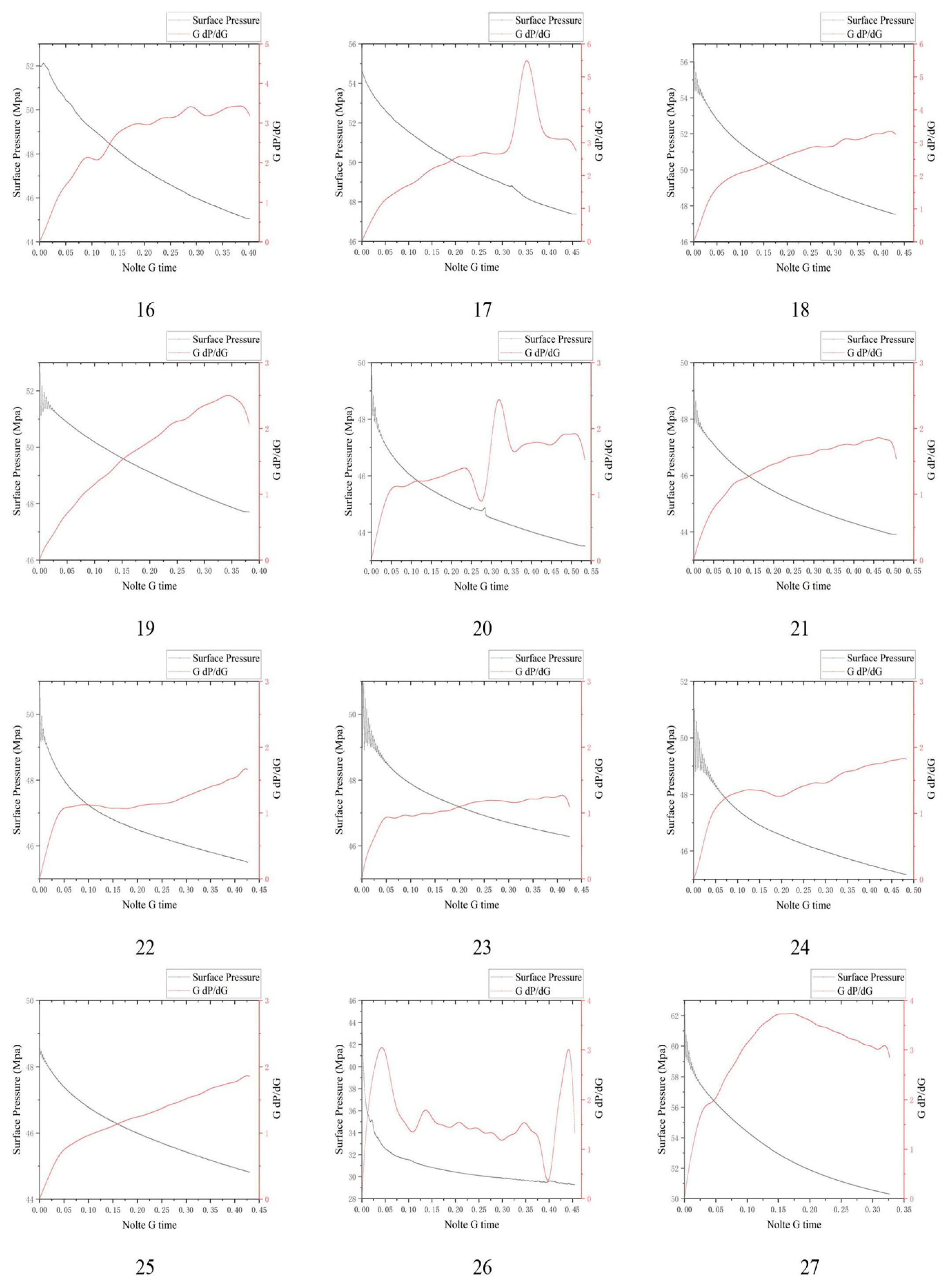
4.1. G-Function Graphic Template Validation

From

Table 2. Production data of some wells in each block.

Block	Serial Number	Well Number	Young’s Modulus (GPa)	Poisson Ratio	Testing Production (104 m3)	Daily Gas Production (m3)	Accumulated Production (104 m3)
I	1	A1	37.4	0.23	14.36	10,862	2716.9
	2	A2	38.38	0.2	32.8	32,145	1237.78
	3	A3	42.1	0.21	12.78	23,644	2684.84
II	4	B1	38.8	0.225	34.28	34,656	1309.79
	5	B2	51.66	0.21	31.7	56,705	2047.5
	6	B3	38.8	0.2	22.7	22,114	544.18
	7	B4	42.6	0.21	20.9	22,266	779.54
III	8	C1	35.5	0.2	19.6	16,590	583.53
	9	C2	44	0.195	9.01	18,868	668.11
	10	C3	44	0.17	7.9	17,318	705.07

, we can see that the wells with a high initial production (≥18 × 10⁴ m³/d) among the 24 wells are A2, B1, B2, B3, B4 and C1. The full-section G-function curves of these six wells were plotted separately and the G-function plates were used as the standard for fast matching as well as verification. Here, only the G-function curves for the full well section of well A2 are listed because of space limitations.

According to the G-function version proposed by the author, the 27 G-function curves in Figure 5 are classified, and the Class I G-function had (1, 2, 3, 6, 8, 11, 16, 17, 18, 20, 26, 27) a total of 12 segments, the Class II G-function had (4, 5, 7, 9, 10, 13, 14, 15, 22) a total of 9 segments, the Class III G-function had (21, 23, 24) a total of 3 segments and the IV type G-function had (12, 19, 25) a total of 3 paragraphs.

The total percentage of G-functions of types I and II was 77.78%, while there were only 6 segments of types III and IV. This shows that most of the segments in well A2 formed complex fracture patterns after hydraulic fracturing, and the fracturing effect was good. From the production data of the A2 well, it has a test production of 328,000 m³/day and a daily production of 32,145 m³, which is the best among the high production wells in this block.

From these 27 segments, we selected four G-function curves that fit into categories I, II, III, and IV, respectively, and analyzed them one by one.

From Figure 6, we can see that a, b, c, and d are consistent with the G-function versions we established for classes I, II, III, and IV, respectively. In this case, we can see from the a-plot that the superimposed derivative of the G-function continues to rise and is accompanied by a large number of fluctuations. In terms of the formed fracture pattern, a complex fracture network including main fractures, branch fractures and a large number of natural fractures was formed.

As we can see in b, the superimposed derivative of the G-function rises rapidly after the pumping stop and then falls back with a lot of fluctuations. In terms of the formed fracture pattern, a complex network of main and branching joints and a small number of natural fractures was formed.

Although fluctuations can be seen in the G-function curve pattern in c, the superimposed derivative of the G-function is less than 2. This represents a smaller fluctuation of the fluid within the fracture after pump stoppage and a simpler fracture pattern. As can be seen in the G-function plots we created, such G-function images corresponded to the fracture morphology of the main fracture plus a large number of natural fractures, which did not form branching fractures of scale.

In subfigure d of Figure 6, the superimposed derivative of the G-function resembles a straight line and no significant fluctuation is seen and is less than 2. Therefore, it represents a poor fracturing effect in this section, where only the main fracture was formed and no branching fracture was formed, and no natural fracture was communicated.

The other five high-producing wells in the block (B1, B2, B3, B4, C1) and low-producing wells (C2, C3) with an initial production below 100,000 m³/day were plotted with the full-section G-function as well as template matching according to the same method, and the results are shown in

Table 3. Matching of G-function plates for high- and low-producing wells in this block.

Category	Well Number	I	II	III	IV	Proportion of Class I and II %
Large-productivity Well	A2	12	9	3	3	77.78
	B1	9	7	5	2	80
	B2	9	7	4	3	69.6
	B3	8	11	2	1	76.2
	B4	7	6	1	1	87.7
Stripper Well	C1	5	11	4	1	76.2
	C2	3	5	15	0	34.8
	C3	0	5	8	10	23.8

.

From Table 3, we can see that the G-function curve types of the high-producing wells in this block conform to the average value of category I and II in the map plate of 77.91%, which represents a good fracturing effect, and all form a complex fracture network, which is consistent with the characteristics of high-producing wells. Meanwhile, most of the G-function curve types of the low-producing wells C2 and C3 in the table are concentrated in categories III and IV in the plate, and the average value of the percentage of the G-function in categories I and II is only 29.3%. The low production was partly due to the fact that no complex fracture network is formed in induced fracturing and the fracture form is single. It can be seen that the G-function plate proposed by the author can accurately match the high and low production capacity after shale fracturing.

In order to further verify the accuracy of the G-function graphic template, the author selected the high-producing section and the low-producing section from the five wells with production profile data in the block and matched the graphic template separately according to the production level. From

Table 4. Matching of G-function plates for high- and low-producing sections of wells in this block.

Category	Well Number	I	II	III	IV	Proportion of Class I and II %
High-yield section	D1	3	3	0	0	100
	D2	3	4	0	0	100
	D3	2	1	0	0	100
	D4	3	2	0	0	100
	D5	2	0	1	1	80
Low-yield section	D1	1	0	1	1	33.3
	D2	1	0	1	2	25
	D3	0	1	1	1	33.3
	D4	1	0	1	1	33.3
	D5	0	0	0	3	0

, it can be seen that the G-functions of the high-yielding section are basically classified in categories I and II, and most of the G-functions of the low-yielding section are classified in categories III and IV. This result can further prove the accuracy and practicality of the plate.

4.2. Validation of the G-Function Yield Evaluation Model

We screened shale gas wells with production profile data and plotted their G-function curves. The relevant parameters were extracted for the high-yielding and low-yielding sections separately, and the parameters included V_ΔPt, k, D and S. After that, we used the extracted parameters to substitute into Equation (11) for the calculation. Note that before calculating the capacity evaluation value Y, we needed to score the extracted parameters using the parameter scoring table in Table 1. The settlement results are shown in

Table 5. Validation of G-function yield evaluation model for high-yield section.

Well Number	Stage Number	Pressure Drop Rate	Initial Slope	Number of Fluctuations	Area under the Curve	VΔPt Score	k Score	D Score	S Score	Evaluation Value Y Score
D1	9	33.3	36	4	0.354	0.75	0.5	0.25	0.75	0.5525
	10	21.41	46.2	6	0.397	0.5	0.75	0.5	0.75	0.66
	19	17.05	46.27	7	0.284	0.25	0.75	0.5	0.5	0.57
	20	21.36	30.69	6	0.198	0.5	0.5	0.5	0.25	0.4625
	22	39.12	117.53	11	0.300	0.75	1	1	0.5	0.8725
	23	30.6	93.64	8	0.086	0.75	1	0.75	0	0.76
D2	3	18.05	30.37	7	0.226	0.25	0.5	0.5	0.5	0.4475
	4	36.39	91.74	6	0.396	0.75	1	0.5	0.75	0.835
	5	23.34	36.32	2	0.435	0.5	0.5	0	0.75	0.4625
	6	27.18	49.01	4	0.326	0.5	0.75	0.25	0.5	0.585
	8	11.64	20	6	0.253	0.25	0.25	0.5	0.5	0.325
	10	30.51	45.89	6	0.392	0.75	0.75	0.5	0.75	0.7125
	11	27.82	31.95	4	0.362	0.5	0.5	0.25	0.75	0.5
D3	13	86.73	404.03	10	0.169	1	1	1	0.25	0.8875
	14	26.39	62.19	6	0.336	0.5	1	0.5	0.5	0.745
	15	69.09	295.58	6	0.110	1	1	0.5	0	0.775
D4	3	16.88	31.5	5	0.338	0.25	0.5	0.25	0.5	0.41
	7	58.07	161.71	9	0.670	1	1	0.75	1	0.9625
	9	80.67	137.82	7	0.203	1	1	0.5	0.5	0.85
	10	74.99	95.04	6	0.121	1	1	0.5	0	0.775
	11	35.65	65.71	3	0.625	0.75	1	0	1	0.7975
D5	15	23.57	52.9	8	0.140	0.5	0.75	0.75	0	0.585
	21	35.69	83.18	6	0.509	0.75	1	0.5	1	0.8725
	10	17.25	36.85	3	0.167	0.25	0.5	0	0.25	0.335

and

Table 6. Validation of G-function yield evaluation model for low-yield section.

Well Number	Stage Number	Pressure Drop Rate	Initial Slope	Number of Fluctuations	Area under the Curve	ΔPt Score	k Score	D Score	S Score	Evaluation Value Y Score
D1	12	23.42	39.71	4	0.532	0.5	0.5	0.25	1	0.388
	18	11.72	23.8	5	0.234	0.25	0.25	0.25	0.5	0.213
	21	23.39	78.59	6	0.217	0.5	1	0.5	0.5	0.67
D2	25	8.71	15.25	2	0.176	0	0.25	0	0.25	0.123
	26	32.8	78.28	7	0.365	0.75	1	0.5	0.75	0.723
	27	36	58.87	4	0.530	0.75	0.75	0.25	1	0.563
D3	1	33.62	38.91	5	0.944	0.75	0.5	0.25	1	0.44
	2	23.03	91.28	9	0.202	0.5	1	0.75	0.5	0.708
	3	31.16	140.26	7	0.352	0.75	1	0.5	0.75	0.723
D4	1	30	30.7	4	0.184	0.75	0.5	0.25	0.25	0.44
	2	12.34	19.76	4	0.279	0.25	0.25	0.25	0.5	0.213
	5	10.28	15.15	4	0.165	0.25	0.25	0.25	0.25	0.213
D5	4	6.35	12.27	4	0.125	0	0	0.25	0	0.038
	5	11.28	18.21	6	0.164	0.25	0.25	0.5	0.25	0.25
	6	12.33	14.25	5	0.159	0.25	0	0.25	0.25	0.09

.

The G-function yield evaluation model proposed by the author was used to identify the G-function curves of the high- and low-yielding segments and to calculate the model. From the calculation results, it can be seen that the average value of the single-segment production evaluation value Y calculated by the G-function curve of the high-production section is 0.656; as a comparison, the average value of the single-segment production evaluation value Y corresponding to the G-function curve of the low-production section is 0.39, which is 59.45% lower than the average value of the Y of the high-production section. In addition, the average values for V_ΔPt and k, which are used to evaluate the fluid flow in the main seam, were 0.63 and 0.8 respectively for the high-yield section. As a comparison, the average values of V_ΔPt and k in the low-yielding section were 0.43 and 0.5, respectively, which were only 68.25% and 62.5% of those in the high-yielding section. In relation to the characteristics of the G-function curves of categories I and II in the G-function plot proposed by the author (fast rising and large upward convex area in the initial stage of the curve), they coincide with V_ΔPt and k in the calculated results, which shows that the established G-function plot has some correlation with the capacity model.

As we can see in Figure 7, the G-function capacity evaluation value for the high-yielding section is significantly lower than that of the high-yielding section, which shows the high accuracy of this model and its practical value.

In summary, our proposed evaluation model can accurately extract data and perform calculations based on G-function curve image features to predict the high or low single-section production after fracturing shale gas wells. This method allows for the immediate post-fracturing effect evaluation at the fracturing construction site so that the fracturing parameters can be optimized and subsequent fracturing construction operations can be performed based on field experience.

5. Conclusions

(1)

Based on the theoretical basis of the G-function, the G-function graphic template and the corresponding fracture pattern were proposed by analyzing the corresponding G-function curve patterns of different blocks in combination with production, and verified according to high- and low-production wells with high accuracy, which can effectively provide feedback on the field fracturing effect and guide the subsequent fracturing construction.

(2)

Based on the morphological characteristics of the G-function curve, a G-function production evaluation mathematical model based on four indicators is proposed and validated using high- and low-producing sections of shale gas wells with production profile data. From the validation of the production capacity model, it can be seen that the average value of the production evaluation Y of the high-producing section is higher than that of the low producing section by 75.9%, which is much larger than that of the low-producing section, which shows the accuracy and adaptability of this model.

(3)

The work intensity at the fracturing site is high and the construction time is long, so it is difficult to have time to evaluate the fracturing effect after completing a section of fracturing construction and to continue the fracturing operation in the next section. Therefore, the author proposes a G-function plate for evaluating the post-fracturing effect, according to which the G-function curve can be quickly matched with the plate after finishing the drawing of the G-function curve to judge the fracture pattern formed after fracturing the section, which is convenient for guiding the efficient construction of fracturing work.

References

1. Dai, J.; Qin, S.; Hu, G.; Ni, Y.; Gan, L.; Huang, S.; Hong, F. Significant progress of natural gas exploration and development in New China over the past 70 years. Pet. Explor. Dev. 2019, 46, 1037–1046. [Google Scholar] [CrossRef]
2. Ma, Y.; Cai, X.; Zhao, P. Theoretical understanding and practice of shale gas exploration and development in China. Pet. Explor. Dev. 2018, 45, 561–574. [Google Scholar] [CrossRef]
3. Ma, X. Theory and practice of unconventional natural gas “limit utilization” development. Pet. Explor. Dev. 2021, 48, 326–336. [Google Scholar] [CrossRef]
4. Zhou, X.; Yong, R.; Fan, Y.; Zeng, B.; Song, Y.; Guo, X.; Zhou, N.; Duan, X.; Zhu, Z. Influence of natural fractures on fracturing of shale gas horizontal wells and process adjustment. China Pet. Explor. 2020, 25, 94–104. [Google Scholar]
5. Zhao, C.; Wang, H.; Guo, W.; Zhang, W.; Fan, Q.; Tian, J.; Chen, H.; Tang, D.; Zhao, J. Shale pneumatic fracture microseismic monitoring technology and its application to Platform X in the Weiyuan area of the Sichuan Basin. Adv. Geophys. 2022, 37, 2089–2096. [Google Scholar]
6. Zhao, C.; Jia, Z.; Tian, J.; Gao, R.; Zhang, W.; Zhao, J. Evaluation of fracturing effect based on in-well microseismic monitoring method—An example of Y22 well in Jilin prospect. Rocky Oil Gas Reserv. 2020, 32, 161–168. [Google Scholar]
7. Zhao, C.; Zhou, Z.; Tian, J.; Li, R.C.; Chang, D.; Zhang, W.; Feng, B.; Li, J. Study on the application of microseismic monitoring in fractured wells of sparse sandstone gas reservoirs: An example from Shibei gas field. Adv. Geophys. 2020, 35, 1919–1925. [Google Scholar]
8. Wang, G.; Xiao, Y.; Zhao, H.; Wang, Y.; Chen, Y. Application of microseismic monitoring technology in repeated fracturing of shale gas horizontal wells. Geol. Explor. 2019, 55, 1336–1342. [Google Scholar]
9. Ren, L.; Su, Y.L.; Xu, C.; Meng, F.K.; Zhan, S.Y. Research progress of capacity prediction methods for volumetric fractured horizontal wells in unconventional reservoirs. In Proceedings of the 2015 International Conference on Oil and Gas Field Exploration and Development, Xi’an, China, 20–21 September 2015; pp. 785–798. [Google Scholar]
10. Rahman, M.K.; Rahman, M.M.; Joarder, A.H. Analytical Production Modeling for Hydraulically Fractured Gas Reservoirs. Liq. Fuels Technol. 2007, 25, 683–704. [Google Scholar] [CrossRef]
11. Rahman, M.M.; Rahman, M.K. Optimizing Hydraulic Fracture to Manage Sand Production by Predicting Critical Drawdown Pressure in Gas Well. J. Energy Resour. Technol. 2012, 134, 013101. [Google Scholar] [CrossRef]
12. Zou, C.; Zhao, Q.; Dong, D.; Yang, Z.; Qiu, Z.; Liang, F.; Wang, N.; Huang, Y.; Duan, A.; Zhang, Q.; et al. Geological characteristics, main challenges and future prospect of shale gas. Nat. Gas Geosci. 2017, 28, 1781–1796. [Google Scholar] [CrossRef]
13. Nolte, K.G. Determination of fracture parameters from fracturing pressure decline. In Proceedings of the SPE Annual Technical Conference and Exhibition, Las Vegas, NV, USA, 23–26 September 1979. [Google Scholar]
14. Nolte, K.G.; Maniere, J.L.; Owens, K.A. After-closure analysis of frac-ture calibration tests. In Proceedings of the SPE Annual Technical Conference and Exhibition, San Antonio, TX, USA, 5–8 October 1997. [Google Scholar]
15. Barree, R.D.; Mukherjee, H. Determination of Pressure Dependent Leakoff and Its Effect on Fracture Geometry. In Proceedings of the SPE Annual Technical Conference and Exhibition, Denver, CO, USA, 6–9 October 1996. [Google Scholar]
16. Meyer, B.R.; Jocat, R.H. Implementation of fracture calibration equations for pressure dependent leakoff. In Proceedings of the SPE/AAPG Western Regional Meeting, Long Beach, CA, USA, 19–22 June 2000. [Google Scholar]
17. Cipolla, C.L.; Warpinski, N.R.; Mayerhofer, M.J. Hydraulic Fracture Complexity: Diagnosis, Remediation, and Exploitation. In Proceedings of the SPE Asia Pacific Oil and Gas Conference and Exhibition, Perth, Australia, 20–22 October 2008. [Google Scholar]
18. Syfan, F.E.; Newman, S.C.; Meyer, B.R.; Behrendt, D.M. Case History: G-function analysis proves beneficial in barnett shale application. In Proceedings of the SPE Annual Technical Conference and Exhibition, Anaheim, CA, USA, 11–14 November 2007. [Google Scholar]
19. Rahman, M.M.; Rahman, M.K.; Rahman, S.S. Multicriteria Hydraulic Fracturing Optimization for Reservoir Stimulation. Pet. Sci. Technol. 2003, 21, 1721–1758. [Google Scholar] [CrossRef]
20. Liu, H.; Gao, Y.; Zheng, L.; Zou, H. Fracturing Net Pressure Diagnoses Modeling for Volcanic Reservoir. In Proceedings of the SPE Asia Pacific Oil and Gas Conference and Exhibition, Perth, Australia, 22–24 October 2012. [Google Scholar]
21. Wang, W.; Zhang, S.; Wang, L.; Zhang, F. Quantitative diagnosis of fracture complexity in bare-hole horizontal wells fractured in volcanic reservoirs. Nat. Gas Ind. 2015, 35, 46–51. [Google Scholar]
22. Zhang, Y.P.; Liu, H. Diagnosis and treatment control of difficult fracturing points in volcanic gas reservoirs. Nat. Gas Ind. 2009, 29, 53–55+143. [Google Scholar]
23. Zhao, W.; Zhang, S.; Sun, Z.; Zhao, Y.; Yang, Y. Research on post-pressure fracture complexity assessment based on G-function curve analysis. Sci. Technol. Eng. 2016, 16, 29–33+45. [Google Scholar]
24. Zhang, C.; Liu, L.; Liu, Q. Research and application of fracturing technology in Songnan volcanic gas reservoir. Drill. Prod. Technol. 2015, 38, 51–54+3. [Google Scholar]
25. Liu, G.; Ehlig-Economides, C. Comprehensive Global Model for Before Closure Analysis of an Injection Falloff Fracture Calibration Test. In Proceedings of the SPE Annual Technical Conference and Exhibition, Houston, TX, USA, 28–30 September 2015. [Google Scholar]
26. Xiao, Y.; Liu, S.; He, Y.; Li, Z.; Wang, J.; Yang, J.; Ma, Z. Evaluation method of fracture complexity of fracture network fracturing in fractured gas reservoirs of dense sandstone. Spec. Oil Gas Reserv. 2022, 29, 157–163. [Google Scholar]
27. Carter, H.W.; Norton, H.W.; Dungan, G.H. Wheat and Cheat1. Agron. J. 1957, 49, 261–267. [Google Scholar] [CrossRef]
28. Liu, G.; Ehlig-Economides, C. Interpretation methodology for fracture calibration test before-closure analysis of normal and abnormal leakoff mechanisms. In Proceedings of the SPE Hydraulic Fracturing Technology Conference, The Woodlands, TX, USA, 9–11 February 2016. [Google Scholar]
Figure 1. The main morphological chart of G-function. (a)Type I, (b) type II, (c) type III, (d) type IV.
Processes 11 01657 g001aProcesses 11 01657 g001b
Figure 2. Fracture morphology corresponding to different types of G-function ((ad) correspond to the crack patterns corresponding to the first, second, third and fourth types of G-functions respectively).
Processes 11 01657 g002
Figure 3. G-function yield evaluation model calculation process.
Processes 11 01657 g003
Figure 4. Example of calculation process. (a) Area Map, (b) grayscale, (c) binarization, (d) Canny edge detection and Hoffman recognition, (e) angle recognition and slope calculation.
Processes 11 01657 g004
Figure 5. G-function curve of A2 well section. (127 are the G-function curves for all segments of shale gas well A2).
Processes 11 01657 g005aProcesses 11 01657 g005b
Figure 6. Example of Class 4 G-function for A2 well. (a) section 2 fracturing, (b) section 4 fracturing, (c) section 23 fracturing, (d) section 25 fracturing.
Processes 11 01657 g006aProcesses 11 01657 g006b
Figure 7. Comparison of evaluation results of high– and low–yield sections.
Processes 11 01657 g007