Abstract
The Fullbore Formation Micro Imager (FMI) represents a proficient method for examining subterranean oil and gas deposits. Despite its effectiveness, due to the inherent configuration of the borehole and the logging apparatus, the micro-resistivity imaging tool cannot achieve complete coverage. This limitation manifests as blank regions on the resulting micro-resistivity logging images, thus posing a challenge to obtaining a comprehensive analysis. In order to ensure the accuracy of subsequent interpretation, it is necessary to fill these blank strips. Traditional inpainting methods can only capture surface features of an image, and can only repair simple structures effectively. However, they often fail to produce satisfactory results when it comes to filling in complex images, such as carbonate formations. In order to address the aforementioned issues, we propose a multiscale generative adversarial network-based image inpainting method using U-Net. Firstly, in order to better fill the local texture details of complex well logging images, two discriminators (global and local) are introduced to ensure the global and local consistency of the image; the local discriminator can better focus on the texture features of the image to provide better texture details. Secondly, in response to the problem of feature loss caused by max pooling in U-Net during down-sampling, the convolution, with a stride of two, is used to reduce dimensionality while also enhancing the descriptive ability of the network. Dilated convolution is also used to replace ordinary convolution, and multiscale contextual information is captured by setting different dilation rates. Finally, we introduce residual blocks on the U-Net network in order to address the degradation problem caused by the increase in network depth, thus improving the quality of the filled logging images. The experiment demonstrates that, in contrast to the majority of existing filling algorithms, the proposed method attains superior outcomes when dealing with the images of intricate lithology.
1. Introduction
Electrical imaging logging is an effective technical tool for reservoir logging evaluation. The two-dimensional image of the well perimeter obtained by using electrical imaging logging can reflect the structure and characteristics of the wellbore wall more intuitively and clearly, addressing geological challenges that cannot be resolved using conventional logging techniques [1,2]. By correlating electrical imaging data with the geological features they reflect, it is possible to identify rock types, as well as divide and compare stratigraphic layers [3,4,5]. Similarly, by combining core data with electrical imaging well logging data, it is possible to directly analyze sedimentary structures, identify sedimentary environments, and distinguish main sedimentary units, revealing provenance and paleo water flow direction [6,7]. However, due to the structure of the well body and the structure of the electrical imaging logging instrument, when scanning along the well wall, the well perimeter coverage cannot reach 100%, and a white band is produced on the electrical logging image [8]. The filling of these blank strips is necessary in order to facilitate the subsequent work of geologists.
Currently, the traditional methods for well log image inpainting can generally be classified into two main categories: structure-based methods and multipoint geostatistical methods, such as the Filtersim algorithm [9,10]. The structure-based filling algorithms are mainly interpolation algorithms, such as inverse distance [11] weighting and Lagrangian interpolation [12]. Jing et al. [11] used the resistivity values of adjacent pole plates between the blank regions in order to interpolate the inverse distance of the blank regions to achieve the information filling of the blank regions. Although this method is simple and fast, the continuity of the filled area with the known area is poor [13]. The interpolation algorithm is simple in principle and fast in processing, but there are obvious traces of processing, and the overall visual effect is poor and cannot meet the actual engineering needs [14]. The Filtersim algorithm [15] is a set of multipoint geostatistical methods based on the principles of filtering. It employs the template-matching principle to “paste” the most similar templates into the target inpainting region, resulting in improved computational efficiency [16]. For example, Hurley et al. [17] applied the Filtersim simulation algorithm from multipoint geostatistics to blank strip filling and achieved good results in logging images of simple stratigraphic structures; Sun et al. [13] applied the inverse distance weighting interpolation method and the multipoint geostatistical Filtersim method to fill the blank strip. However, due to the sequential simulation used by the Filtersim algorithm in filling, which has a stochastic nature, the results are not good after filling the multilayered rational regions where structural features dominate.
With the continuous research and development of deep learning theory in recent years, the advantages of convolutional neural networks in image processing have gradually emerged [18,19]. Owing to the powerful ability of neural networks to capture image information, some successful applications have been achieved in image processing [20,21,22,23]. In recent years, researchers have gradually applied neural networks to the processing of electrical imaging logs. For example, Wang et al. [24] preliminarily applied neural networks to image completion in electric logging, drawing on the idea of deep neural network structures designed by humans to capture a large amount of prior statistical information about bottom-level images [25]. They constructed an encoder–decoder network model, which extracts features through the encoding layer and restores the image through the decoding layer. However, because of the simplicity of the applied model, the filling effect of electric logging images was not ideal. Zhang et al. [26] also utilized the U-Net network to complete electric logging images, which improved the filling effect to some extent. However, for intricate sand and gravel imagery, the contour information cannot be suitably reconstructed, thereby engendering an inadequate filling outcome. Du et al. [27] extended Wang’s [24] approach by incorporating attention mechanisms to constrain the feature extraction process, enabling a focus on important features and resulting in further enhancement of the filling effect.
Drawing upon the literature examined previously, it can be observed that the application of neural network technology in blank interval filling methods is relatively limited, and the targeting is not sufficiently strong. After an extensive literature review, it was found that generative adversarial networks (GANs) [28] have found extensive applications in the domain of image generation. Thanks to their ability to simulate complex functional relationships and their powerful generation capabilities, several papers have used GANs to process image data and have achieved good results [29,30,31,32]. Residual Network (ResNet) [33] is another highly influential network following the three classic CNNs: AlexNet, VGG, and GoogleNet. Owing to its simplicity and practical advantages, ResNet has been widely used in fields such as detection, classification, and recognition [34,35,36,37]. Dilated Convolution [38,39] has been demonstrated to enhance the modeling capacity of deep learning neural networks more effectively for geometric transformations. The dilated convolution operation has the advantage of being able to capture a larger receptive field compared to traditional convolutions, thereby preserving the spatial features of the image well without sacrificing image detail information [40].
In order to address the problem of filling blank strips in structurally complex electrical imaging, we propose a method for filling the blank strips in electrical imaging images based on multiscale generative adversarial network architecture and apply this method to fill the blank strips in complex electrical imaging images. The major contributions are outlined as follows:
- The proposed method utilizes generative adversarial network architecture with U-Net as the generator to enhance the feature extraction capability of the network. In addition, two discriminators, i.e., global and local discriminators, are introduced to capture the overall image and local texture information of complex electrical imaging, respectively, which leads to better texture details in the completed image.
- The introduction of residual networks enhances gradient propagation and addresses the issue of network degradation with increasing depth, thereby improving the quality of the electrical imaging image filling.
- The use of dilated convolution instead of conventional convolution in neural networks helps to better preserve the spatial features of the image, thus improving the reconstruction of complex electric logging images, especially in terms of contour features.
Based on the experimental results, it can be inferred that the image filled by the network model proposed by us is more consistent with the contextual content, and shows significant improvements in the details and textures of the image compared to traditional filling methods and basic deep generative networks.
2. Construction of the Blank Strip Filling Model
2.1. Improved U-Net-Based Model
The deep generative network model we used for blank strip filling in logging electrical imaging is shown in Figure 1. The model is based on GAN architecture, consisting of two main modules: a generator and a discriminator.
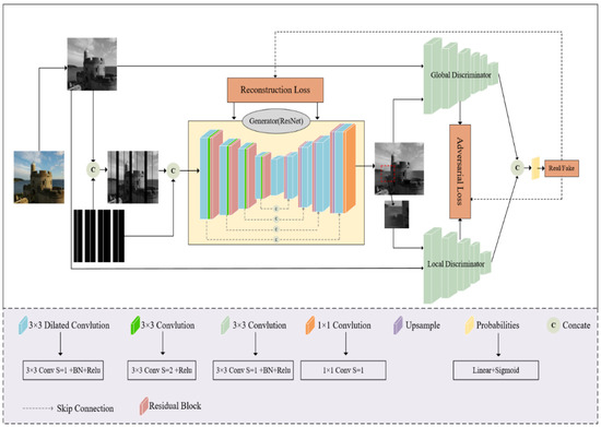
Figure 1.
The network architecture diagram of the blank stripe filling model.
The generator is based on encoder–decoder network architecture. The encoder consists of five modules, each of which is composed of a convolutional layer, batch normalization layer, Rectified Linear Unit (ReLU) activation function, and residual network connection layer. The introduction of a residual network simplifies the learning process, enhances gradient propagation, and solves the degradation problem of the network, caused by increasing depth of the network, thereby further improving the quality of image inpainting. The specific structure is shown in Figure 2. The encoder employs a 3 × 3 convolution kernel, and replaces pooling layers by using convolutional layers with a stride of 2 for down-sampling. Batch normalization layers are added in order to alleviate the problem of “vanishing/exploding gradients” in the network. The decoder part consists of four modules, each of which is composed of an up-sampling layer, a skip connection layer, a convolution layer, a normalization layer, an activation function layer, and a residual connection layer. The up-sampling scale of the decoding layer is 2, with a convolution kernel size of 3 × 3 and a stride of 1.
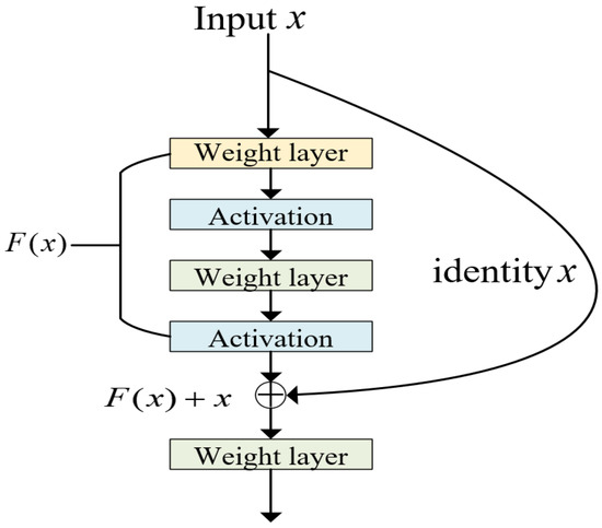
Figure 2.
The network architecture of ResNet and the short connection.
The discriminator consists of two modules: a global discriminator and a local discriminator. The global discriminator has 5 modules, where the first 4 modules consist of convolutional layers, batch normalization layers, and ReLU activation functions, and the last module consists of a Flatten layer, fully connected layer, and Sigmoid activation function. The local discriminator has the same architecture as the global discriminator. The global discriminator evaluates the entire image from a global perspective, while the local discriminator focuses more on the details of the image to provide better image details. Alternating training between the generator and discriminator can improve the quality of image inpainting.
In order to achieve better inpainting results, we modified the convolution method in the encoder–decoder section by introducing dilated convolutions with which to replace regular convolution layers. This increases the receptive field to better handle variations in image details, optimizing the model structure and enabling inference of texture feature information for a single image.
2.2. Residual Network Structure
ResNet was proposed by Kaiming He in 2015. At that time, it was widely believed that deeper neural networks would lead to better performance. However, researchers found that increasing network depth actually led to worse performance, known as the problem of network degradation, and gradient vanishing was identified as a key factor. ResNet provided a solution to this problem by introducing residual connections and achieved excellent results in the 2015 ImageNet image recognition challenge, which had a profound impact on the subsequent design of deep neural networks.
As is widely recognized, in the context of convolutional neural networks (CNNs), the matrix representation of an image serves as its most fundamental feature, which is utilized as the input to the CNNs. The CNNs function as information extraction processes, progressively extracting highly abstract features from low-level features. The greater the number of layers in the network, the greater the number of abstract features that can be extracted, which consequently yields more semantic information. In the case of conventional CNNs, augmenting the network depth in a simplistic manner can potentially trigger issues such as vanishing and exploding gradients. The solutions to the problems of vanishing and exploding gradients usually involve normalized initialization and intermediate normalization layers. However, this can lead to another problem—the degradation problem—in which, as the network depth increases, the accuracy of the training set saturates or even decreases. This is dissimilar to overfitting, which generally exhibits superior performance on the training set.
ResNet proposed a solution to address network degradation. In the event that the subsequent layers of a deep network are identity mappings, the model would experience a decline in performance to that of a shallow network. Therefore, the challenge now is to learn the identity mapping function. However, it is challenging to directly fit some layers to a potential identity mapping function , which is likely the reason why deep networks are difficult to train. In order to address this issue, ResNet is designed with , as shown in Figure 2. We can transform it into learning a residual function, . As long as , it constitutes an identity mapping . Here, is the residual, for which fitting is undoubtedly easier.
ResNet offers two approaches to addressing the degradation problem: identity mapping and residual mapping. Identity mapping refers to the “straight line” portion in the Figure 2, while residual mapping refers to the remaining “non-straight line” portion. represents the pre-summing network mapping, while represents the post-summing network mapping of the input . In order to provide an intuitive example, suppose we map 5 to 5.1. Before introducing the residual, we have . After introducing the residual, we have , where and . Both and represent network parameter mappings, and the mapping after introducing the residual is more sensitive to changes in the output. For example, if the output s changes from 5.1 to 5.2, the output of the mapping increases by 2% (i.e., 1/51). However, for the residual structure, when the output changes from 5.1 to 5.2, the mapping changes from 0.1 to 0.2, resulting in a 100% increase. It is evident that the change in output has a greater effect on adjusting the weights for the latter, resulting in better performance. This residual learning structure is achieved through forward neural networks with shortcut connections, where the shortcut connection performs an equivalent mapping without introducing extra parameters or elevating computational complexity. The entire network can still be trained end-to-end through backpropagation.
2.3. Dilated Convolution
The convolutional modules used in conventional convolutional neural networks have a fixed structure, which limits their ability to model geometric transformations [40]. As a result, when applied to images of sandstone with complex structures and textures, the performance is often poor. In order to address this issue, we employ dilated convolution to replace the regular convolutional layers, optimizing the network model and improving its ability to model geometric transformations.
Typical convolutional neural network algorithms commonly leverage pooling and convolution layers to expand the receptive field, while also reducing the resolution of the feature map. Subsequently, up-sampling methods such as deconvolution and unpooling are used to restore the image size. Due to the loss of accuracy caused by the shrinking and enlarging of feature maps during the down-sampling and up-sampling process, there is a need for an operation that can increase the receptive field while maintaining the size of the feature map. This operation can replace the down-sampling and up-sampling operations. In response to this need, the dilated convolution was introduced.
Different from normal convolution, dilated convolution introduces a hyperparameter called the “dilation rate”, which defines the spacing between values in the convolution kernel when processing the data. From left to right, Figure 3a–c are independent convolution operations. The large boxes represent the input images (with a default receptive field of 1), the black circles represent 3 × 3 convolution kernels, and the gray areas represent the receptive field after convolution. Figure 3a represents the normal convolution process (with a dilation rate of 1), resulting in a receptive field of 3. Figure 3b represents the dilation rate of 2 for the dilated convolution, resulting in a receptive field of 5. Figure 3c represents the dilation rate of 3 for the dilated convolution, resulting in a receptive field of 7.
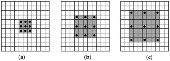
Figure 3.
Illustration of Receptive Fields of Dilated Convolutions with Different Dilation Rates: (a) represents the receptive field when the dilation rate is 1; (b) represents the receptive field when the dilation rate is 2; (c) represents the receptive field when the dilation rate is 3.
From Figure 3, it can be seen that with the same 3 × 3 convolution, the effect of convolutions equivalent to 5 × 5, 7 × 7, etc., can be achieved. Dilated convolutions possess the ability to enlarge the receptive field, whilst avoiding an increase in the number of parameters (number of parameters = convolutional kernel size + bias). Assuming the convolutional kernel size of the dilated convolution is and the dilation rate is , then its equivalent convolutional kernel size can be calculated using the following formula, for example, for a 3 × 3 convolutional kernel, = 3:
The formula involves several parameters: “” denotes the dimensions of the output feature map, “” denotes the size of the input feature map, denotes the equivalent kernel size computed in the first step, stride denotes the step size, and padding denotes the size of the padding. Usually, the padding size is designed to be the same as the dilation rate in order to ensure that the output feature map size remains unchanged. However, simply stacking dilated convolutions with the same dilation rate can cause grid effects, as shown in Figure 4.
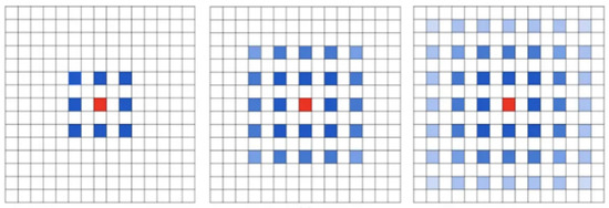
Figure 4.
The grid effect of dilated convolution.
As shown in Figure 4, stacking multiple dilated convolutions with a dilation rate of 2 can lead to the problem reflected in the figure. It is evident that the kernel exhibits discontinuity, thereby implying that not all pixels are involved in the computation, and thus leading to a reduction in the continuity of information. In order to address this issue, Panqu Wang proposed the design principle of HDC (Hybrid Dilated Convolution). The solution is to design the dilation rates in a zigzag structure, such as [1,2,5], and satisfy the following formula:
The variable represents the dilation rate for layer and represents the maximum dilation rate in layer , assuming n total layers and = by default. If we use a kernel of size , our goal is to ensure that ≤ , so that all the holes can be covered using dilation rate 1, which is equivalent to standard convolution.
3. The Algorithm of Blank Stripe Filling Based on Multiscale Generative Adversarial Network
3.1. Algorithm Principle
Current deep neural network-based image restoration methods typically require a large amount of training data [41], a requirement which is not suitable for filling the blank strips in well logging electric images. For electrical imaging logging, it is impossible to obtain a complete image of the formation, and obtaining a large amount of image data of the wellbore and surrounding wells is also a significant challenge in engineering. Ulyanov et al. [25] pointed out that neural network architectures themselves can capture low-level statistical distributions, and that the original image can be restored using only the corrupted image. Building upon this idea, this paper minimizes the function by optimizing the deep convolutional network model parameters , and implements the filling of blank strips through alternating training of the generator and discriminator. The specific algorithmic principle is shown in Figure 5.
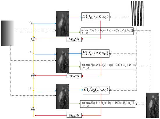
Figure 5.
The schematic diagram of the blank stripe filling network algorithm.
In Figure 5, the leftmost image represents the input to the network model, which is initialized with randomly initialized model parameters . The network output is obtained from input z through the function . The image is used to calculate the loss term for the filling task, and is input together with the original image into the discriminative network to calculate the GAN loss. Here, represents the discriminant function, is a random mask used to randomly select an image patch for the local discriminator, represents the generative network function, and represents the missing area. We aim for the discriminator to not be able to distinguish between the generated images and the real original images, thus obtaining a complete image with realistic texture details. The loss gradient is computed using the gradient descent algorithm to obtain new weights and this process is repeated until the optimal is found. Finally, the complete image is obtained using the formula .
3.2. Algorithm Flow
Step 1: Generating mask images.
In order to simulate the missing data in real well logging images, we generate corresponding masks by scanning the real electric well logging images. As modern electrical imaging logging software typically sets blank areas in the image data as a constant value when converting data from electrode measurements to image data, the pixel values of blank areas are fixed. Therefore, we implement the detection of blank areas in electrical imaging logging images through a point-by-point scanning method using PyCharm software. The RGB pixel values of the scanned blank areas are set to (255, 255, 255), and the pixel values of other non-blank areas are set to (0, 0, 0), thus obtaining the mask image of the logging image. The original logging image and its corresponding mask image are shown in Figure 6.
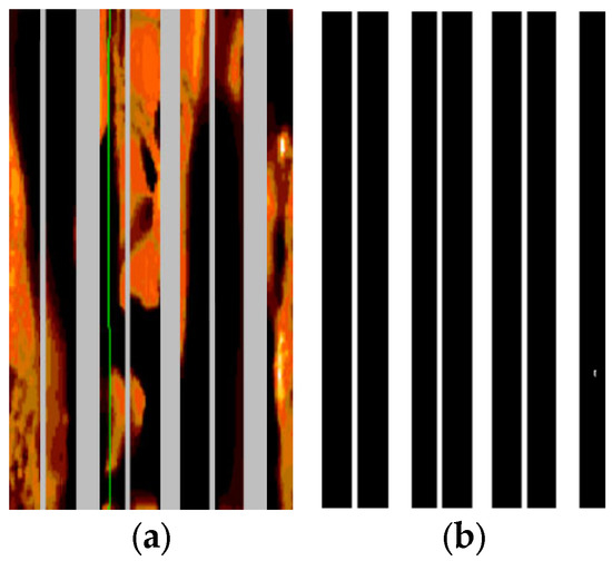
Figure 6.
Log image and its corresponding mask image: (a) log image and (b) mask image.
Step 2: Generating the image to be filled.
To ensure that colors outside of the electrical imaging scale bar do not appear after filling, this paper converts the electrical imaging log image to grayscale as the image to be filled, and the output of the network model is also a 1-channel grayscale image. The grayscale image is subtracted from the original grayscale image and multiplied by its corresponding mask to obtain the image to be filled, as shown in Figure 7.
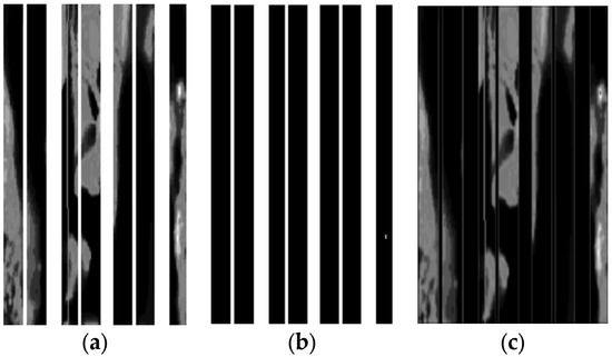
Figure 7.
Grayscale image of the electric logging to be filled in: (a) the original grayscale image; (b) mask image; and (c) image to be filled.
Step 3: Training of the generative network.
For the training of the generative network, we utilized the Places365-Standard dataset [42]. This dataset comprises approximately 1.8 million images, covering 365 distinct scene categories, such as beaches, forests, offices, kitchens, and more. The images in the dataset were collected from the internet, resulting in a wide range of visual diversity and complexity. The image sizes vary from as low as a few tens of kilobytes to as high as several tens of megabytes. This characteristic makes Places365-Standard a challenging dataset suitable for evaluating and training machine learning models in real-world scenarios. To obtain Places365-Standard dataset, it can be downloaded from its official website.
From the dataset, we randomly selected 30,000 images for the training set and 6000 images for the validation set. These images were preprocessed and cropped to a uniform size of 256 × 256 pixels, and the to-be-filled images were produced using the methods from the previous two steps. The output data of the generative network, i.e., the filled grayscale image and the input grayscale image with the mask image, were multiplied, and the mean squared error (MSE) of the pixel values in the missing regions was calculated. The formula for MSE loss is as follows:
In the formula, represents the number of pixels, represents the output of the generative network, and represents the original image.
The MSE function has a smooth and continuous curve that is differentiable everywhere, making it suitable for use with gradient descent algorithms, and is a commonly used loss function. Additionally, as the error decreases, the gradient also decreases, which is conducive to convergence. Even with a fixed learning rate, it can converge quickly to the minimum value. The Adam stochastic gradient descent (SGD) optimization algorithm was used to train the generative network and update the parameter . Thereafter, we updated the network parameters through the backpropagation of the generation model. The training process was repeated until the loss value reached an acceptable range.
Step 4: Training of the discriminative network.
After the training of the generative network is completed, a randomly cropped section of the generative network output is used as the input for the local discriminator, while the entire generated image is used as the input for the global discriminator. During the training of the discriminator, the binary cross-entropy (BCE) is used as the loss function.
The utilization of the BCE loss facilitates the discriminator in effectively distinguishing between real and generated samples. By minimizing the BCE loss, the discriminator gradually improves its classification ability, thereby enabling the generator to produce more realistic samples, which is formulated as follows:
In the formula, represents the binary label of 0 or 1, and represents the probability that the output belongs to the y label. The discriminator is trained by feeding both the original and generated images produced by the generative network into the discriminative network, and the binary cross-entropy (BCE) loss is computed. This process is repeatedly performed until the loss value reaches an acceptable range. We hope that the discriminator cannot distinguish between complete images and real images, thereby obtaining complete images with realistic texture details.
Step 5: Training the generative and discriminative networks jointly.
After the discriminative network is trained, a joint loss function is used to alternately train the generative network and the discriminative network. The joint loss function is shown as follows:
In the formula, is a weighted hyperparameter used to balance the MSE loss and GAN loss. In this step, we first train the discriminative network to correctly distinguish between the completed images and the real images. Thereafter, the generative network is trained to generate results that cannot be distinguished as fake by the discriminative network. We repeat this alternating training process between the discriminative and generative networks until the loss values reach an acceptable range.
Step 6: Generation of final images.
After the entire training process is completed, we only need to use the generative network to input the incomplete image and obtain the completed image. The output image at this time is still a 1-channel grayscale image, which is eventually converted to a color image by comparing the grayscale values on the electric imaging scale, thereby completing the filling task of electric imaging well logging.
In order to facilitate a better understanding of the key steps and logic of the algorithm, we have included a pseudocode representation of the algorithm, as shown in Algorithm 1. This pseudocode serves as a concise and structured description of the algorithm’s implementation, enabling readers to grasp its essential components and flow more readily.
| Algorithm 1 Training procedure of the ResGAN-Unet |
| 1: while iterations < do |
| 2: Sample a minibatch of images from training data. |
| 3: Input masks for each image in the minibatch. |
| 4: if < then |
| 5: Update the generation with the weighted MSE |
| Loss (Equation (4)) using (). |
| 6: else |
| 7: Generate masks with random hole for each |
| image in the minibatch. |
| 8: Update the discriminators with the binary cross |
| entropy loss with both ((),) and (). |
| 9: if > + then |
| 10: Update the generative network with the |
| joint loss gradients (Equation (6)) using (), and . |
| 11: end if |
| 12: end if |
| 13: end while |
In Algorithm 1, “” denotes the total number of iterations for the network, while “” and “” respectively denote the iteration counts for the generative network and the discriminative network.
4. Experimental Results and Analysis
4.1. Experimental Environment
The network model proposed in this paper was implemented in a PyTorch deep learning framework and run on an NVIDIA RTX A5000 GPU server with a virtual environment configured with Python 3.9 and CUDA 11.6. The batch size during training was set to 8, and the Adam optimizer [43] was used with a learning rate of 0.001. The experiment was iterated 5000 times.
4.2. Experiment on Natural Image Inpainting
In order to validate the effectiveness of the proposed algorithm, we first conducted image inpainting experiments on missing natural images.
4.2.1. Introduction to the Dataset
For the natural image experiment, the testing dataset used is still the Places365-Standard dataset. We randomly selected 10 images from the dataset as the original images for this paper’s experiment. In order to make the experimental results more convincing, we used strip masks similar to those in logging-while-drilling during the experiments.
One of the natural images utilized for the experiment in this paper is depicted in Figure 8, where Figure 8a is the original image in the dataset. We converted the color image to a grayscale image for processing, as shown in Figure 8b, while Figure 8c represents the mask image used in the filling experiment, where white areas denote missing parts of the image, and black areas denote preserved image information. The original image subtracted from the corresponding pixel-wise multiplication of the original image with the mask image is used as the image to be filled in the experiment, as shown in Figure 8d.
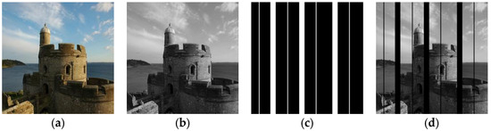
Figure 8.
Example of natural image to be inpainted: (a) original image; (b) grayscale image; (c) mask image; and (d) inpainting image.
4.2.2. Experimental Results and Analysis
The filling results of the example image in Figure 8, using four different network models, are shown in Figure 9. We can observe from Figure 9 that the conventional encoder–decoder network (Figure 9a) [16] shows obvious filling traces, as indicated by the red dotted lines. Compared to Figure 9a, the use of the U-Net network structure Figure 9b brings some improvement to filling traces, but pixel loss is still severe. With the Res-Unet network and the addition of dilated convolutions (Figure 9c), the pixel loss issue is significantly improved, as indicated by the dotted lines in the figure, and the overall filling quality of the image is improved. After incorporating two discriminators into the base model (Figure 9c) to form a GAN (Figure 9d), the details of image inpainting have been improved, as is evident in the marked regions. The filling results of the strip edges have been significantly enhanced, leading to a notable improvement in overall performance.
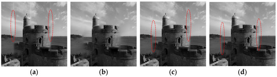
Figure 9.
Natural image inpainting results: (a) filling result of the basic encoder–decoder network; (b) filling result of the U-Net network; (c) filling result of the Res-Unet network; and (d) filling result of the ResGAN-Unet network.
Further quantitative analysis was conducted on the experimental results by calculating evaluation metrics, such as SSIM (Structural Similarity Index), PSNR (Peak Signal-to-Noise Ratio), MSE (Mean Squared Error), and FID (Fréchet Inception Distance) for both the 10 original images and the corresponding generated images using the proposed models. The average results for each metric across the 10 images are shown in Table 1. From the table, it can be observed that the proposed algorithm consistently outperforms the conventional model methods, thereby validating the advantages of the proposed models.

Table 1.
Comparison of Evaluation Metrics for Image Inpainting Results using Different Models.
Here, SSIM is a structured image quality evaluation index that measures the structural similarity between two images. The closer the SSIM value is to 1, the higher the similarity with the original image. PSNR, or peak signal-to-noise ratio, is the most widely used objective image quality evaluation index, where a larger value indicates less distortion. MSE represents the mean square error between the current image X and the reference image Y, with a higher value indicating more severe image distortion. In order to evaluate the metrics of GAN-generated images, a new metric called Fréchet Inception Distance (FID) has been introduced. FID quantifies image quality by comparing the feature distributions of generated images and real images. A smaller FID value indicates that the generated images are closer to the real images in terms of their features and distributions, demonstrating higher realism and fidelity.
As shown in Table 1, the values of SSIM and PSNR increase gradually, while the value of MSE and FID decreases gradually, indicating that the network model’s filling effect is becoming better and better.
4.3. Experiment on Electrical Logging Image Inpainting
4.3.1. Introduction to the Dataset
Regarding the well log image dataset, we employed actual recorded electric imaging images from a logging company, specifically from Well C2 in the Bo Block, located approximately 700 m underground. This dataset encompasses a variety of well log images with different types of color calibration, including both dynamic and static color scales.
4.3.2. Experimental Results and Analysis
The filling results of two logging images are shown in Figure 10. The two original logging images are shown in Figure 10a, and the corresponding filling results using the basic encoder–decoder network are shown in Figure 10b. From the filling results, it can be observed that both the upper and lower images in Figure 10b show filling traces, as marked by the blue dashed lines. The continuity of the texture in the images is poor, and there is a clear sense of boundary, indicating an overall poor performance, which is not conducive to subsequent geological work.
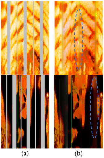
Figure 10.
Image filled by basic model: (a) shows the original electrical resistivity well logging image; (b) shows the final image after being filled using the basic encoder–decoder network.
In order to improve the filling quality of well logging images, firstly, the conventional neural network structure was replaced with a U-Net network structure in the basic encoder–decoder network. Secondly, in the U-Net network, residual blocks were added and the original convolutional layers were replaced with dilated convolutions. Lastly, two discriminators were further introduced to form a generative adversarial network structure on the previous network. The experimental results are shown in Figure 11.
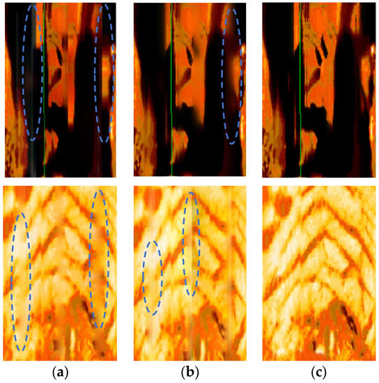
Figure 11.
Comparison of filling results of different improved network models: (a) filling result of the U-Net network; (b) filling result of the Res-Unet network; and (c) filling result of the ResGAN-Unet network.
The filling results obtained by replacing the basic encoder–decoder structure with the U-Net network structure are illustrated in Figure 11a. It can be seen that, compared with the original network, the filling effect has been improved to some extent. The continuity of the image texture has been enhanced, and the filling traces at the edge of the overall blank strip have been improved. However, there are still filling traces, as indicated by the blue dotted line in the figure.
The filling results are displayed in Figure 11b after residual networks and dilated convolutions were introduced on U-Net structure. The results show that the introduction of residual networks significantly improves the filling trace of blank strips, enhances the clarity of boundaries between different structures in the image, and makes the filling of the same structure more natural. This indicates that the introduction of residual networks helps to capture the overall structural information of the image, resulting in more accurate filling. However, there are still some shortcomings in the filling results regarding some details, as marked in Figure 11b.
The filling results of the generative adversarial network (GAN), composed of U-Net and residual network structures with both global and local discriminators, are shown in Figure 11c. From the result in Figure 11c, it can be observed that the filling effect of the image has reached its optimal level after training the GAN. The filling traces of the overall blank stripe have become barely distinguishable, which indicates that the multiscale discriminators can provide good texture details of the complete image at different scales. After training with the two discriminators, the filling of the details in the image has been significantly improved, thereby further enhancing the overall visual effect, which is beneficial to the subsequent work of formation division and lithology detection.
The filling results of three additional electrical logging images are shown in Figure 12. The original well logging images before filling are represented by Figure 12a, while the best filling results obtained using other models are displayed in Figure 12b. The corresponding filling results obtained using the proposed model in this paper are shown in Figure 12c. From these images, it can be observed that, for relatively simply structured images, such as the first and third images in Figure 12a, the results obtained by other models are acceptable. However, for complex-structured images, such as the second image, the filling results achieved by the proposed method in this paper are significantly superior to those of other models. They can accurately and realistically fill the missing content in the blank intervals, with almost imperceptible traces at the edges of the intervals. Overall, the visual effect of the filled images has been greatly improved.
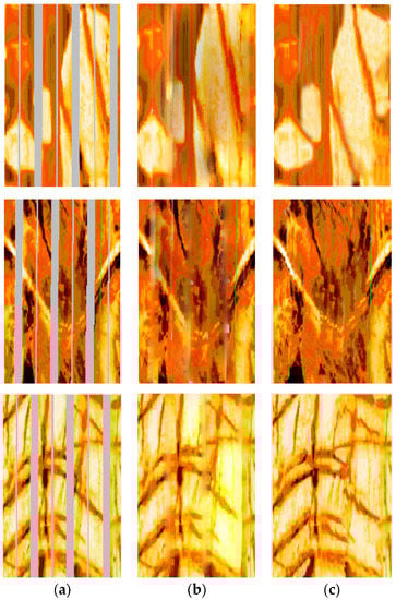
Figure 12.
Demonstration of final filling results of other logging images: (a) the original image; (b) the best results obtained by applying other models for filling; and (c) the results obtained by applying the model proposed in this paper for filling.
5. Conclusions
In order to address the issue of filling in blank strips in complex well logging images, we improved the basic encoder–decoder network in the U-Net architecture by simultaneously introducing residual networks and multiscale discriminators. By learning a large number of examples of filling blank bands, and through network model calculation based on the original image and marked area to be filled, the filling of blank bands was achieved. The improved model was used to conduct image inpainting experiments on natural images and complex well logging images. Both experiments demonstrated that the proposed deep learning network can effectively fill in missing data in images, and outperforms conventional encoder–decoder networks in metrics, such as SSIM, PSNR, MSE and FID. This indicates that:
- (1)
- The introduction of residual networks helps to preserve the integrity of information and solve the problem of network degradation. It better captures the overall structure of the image and, thus, more accurately fills in the overall content of the image;
- (2)
- The incorporation of the multiscale discriminator ensures the global and local consistency of the image. The global discriminator is better at filling in the overall image in a global sense, while the introduction of a local discriminator better fills in the texture details of the image.
After conducting experiments on multiple electric imaging well logging images, the results show that the algorithm proposed in this paper can effectively fill the blank strips of complex electric imaging well logging images. The filling traces are barely noticeable, and the image exhibits good continuity and texture, with clear edge contours, which is beneficial for professional geological interpretation in the later stage. The proposed algorithm provides technical support for actual exploration in well logging. For instance, it aids geologists in efficiently identifying distinct geological layers and lithologies, as well as inferring underground geological structures and structural characteristics. Additionally, in tasks such as deep learning-based stratigraphic segmentation, it facilitates the work of geology experts in conveniently and accurately annotating datasets, thereby establishing a solid foundation for model training.
Nevertheless, in the research of filling blank strips in electrical well logging, there are still challenges to be addressed, such as dealing with complex geological structures, improving the stability and robustness of filling results, etc. Future research on filling blank strips in electrical well logging can incorporate more geological information in order to enhance the filling effectiveness. For example, introducing stratigraphic information and rock distribution models can help achieve more realistic geological representation in the filling results. Therefore, it is necessary to explore new algorithms and methods in order to further improve the accuracy and reliability of filling blank intervals in electrical well logging.
Author Contributions
Conceptualization, Q.S. and N.S.; methodology, N.S.; software, N.S. and Q.S.; validation, N.S.; formal analysis, N.S. and F.G.; investigation, Q.S. and N.S.; data curation, N.S.; writing—original draft preparation, N.S.; writing—review and editing, Q.S. and Q.D.; visualization, N.S.; supervision, Q.S. and Q.D.; funding acquisition, Q.S., F.G. and Q.D. All authors have read and agreed to the published version of the manuscript.
Funding
This research was funded by the National Natural Science Foundation of China, grant number 41930429, and the CNPC Major Science and Technology Project (ZD2019-183-006).
Data Availability Statement
Not applicable.
Acknowledgments
We would like to thank the reviewers for their valuable comments to improve the quality of the paper.
Conflicts of Interest
The authors declare no conflict of interest.
References
- Hassan, S.; Darwish, M.; Tahoun, S.S.; Radwan, A.E. An integrated high-resolution image log, sequence stratigraphy and palynofacies analysis to reconstruct the Albian–Cenomanian basin depositional setting and cyclicity: Insights from the southern Tethys. Mar. Pet. Geol. 2022, 137, 105502. [Google Scholar] [CrossRef]
- Gao, J.; Jiang, L.; Liu, Y.; Chen, Y. Review and analysis on the development and applications of electrical imaging logging in oil-based mud. J. Appl. Geophys. 2019, 171, 103872. [Google Scholar] [CrossRef]
- Zhang, Z.B.; Xu, W.; Liu, Y.H.; Zhou, G.Q.; Wang, D.S.; Sun, B.; Feng, J.S.; Liu, B. Understanding the Complex Channel Sand Reservoir from High-Definition Oil-Base Mud Microresistivity Image Logs: Case Study from Junggar Basin. In Proceedings of the Offshore Technology Conference, Houston, TX, USA, 2–5 May 2022. [Google Scholar]
- Zhou, F.; Oraby, M.; Luft, J.; Guevara, M.O.; Keogh, S.; Lai, W. Coal seam gas reservoir characterisation based on high-resolution image logs from vertical and horizontal wells: A case study. Int. J. Coal Geol. 2022, 262, 104110. [Google Scholar] [CrossRef]
- Luo, X.; Pang, X.; Dongxu, S.U.; Hui, L.U.; Zhang, N.; Wang, G. Recognition of Complicated Sandy Conglomerate Reservoir Based on Micro-Resistivity Imaging Logging: A Case Study of Baikouquan Formation in Western Slope of Mahu Sag, Junggar Basin. Xinjiang Pet. Geol. 2018, 39, 1. [Google Scholar]
- El-Gendy, N.H.; Radwan, A.E.; Waziry, M.A.; Dodd, T.J.; Barakat, M.K. An integrated sedimentological, rock typing, image logs, and artificial neural networks analysis for reservoir quality assessment of the heterogeneous fluvial-deltaic Messinian Abu Madi reservoirs, Salma field, onshore East Nile Delta, Egypt. Mar. Pet. Geol. 2022, 145, 105910. [Google Scholar] [CrossRef]
- Zhang, C.; Fan, T.; Meng, M.; Jun, W.U. Geological Interpretation of Ordovician Carbonate Reservoir in Tahe Oilfield: Application of Imaging Logging Technology. Xinjiang Pet. Geol. 2018, 39, 1. [Google Scholar]
- Ni, L.Q.; Xu, H.Q.; Li, Q.W.; Li, G.J.; Xu, C.H. Ultrasonic Logging Image Restoration Based on Texture. Well Logging Technol. 2010, 34, 4. [Google Scholar]
- He, K.; Lu, W.X.; Shen, C.N.; Huang, W.R. Exemplar-Based Inpainting Algorithm with Rotation and Scaling Transformation. Laser Optoelectron. Prog. 2018, 55, 031006. [Google Scholar]
- Ma, P.S.; Li, S.H.; Lu, C.S.; Huang, D.W.; Duan, D.P.; Lu, Y.; Ding, F.; Huang, X. Multi-point geostatistical method based on mode method clustering. J. Nat. Gas Geosci. 2020, 31, 9. [Google Scholar]
- Jing, M.; Wu, J. Fast image interpolation using directional inverse distance weighting for real-time applications. Opt. Commun. 2013, 286, 111–116. [Google Scholar] [CrossRef]
- Occorsio, D.; Ramella, G.; Themistoclakis, W. Lagrange–Chebyshev Interpolation for image resizing. Math. Comput. Simul. 2022, 197, 105–126. [Google Scholar] [CrossRef]
- Sun, J.M.; Zhao, J.P.; Lai, F.Q.; Chen, H. Methods to Fill in the Gaps Between Pads of Electrical Logging Images. Well Logging Technol. 2011, 35, 532–537. [Google Scholar]
- Jini, P.; Rajkumar, K. Image Inpainting Using Image Interpolation—An Analysis. Rev. Geintec-Gest. Inov. E Tecnol. 2021, 11, 1906–1920. [Google Scholar]
- Zhang, T.F. Filter-Based Training Pattern Classification for Spatial Pattern Simulation. Ph.D. Thesis, Stanford University, Stanford, CA, USA, 2006. [Google Scholar]
- Zhang, T. Reconstruction Method and Implementation of Porous Media Based on Multi-Point Geostatistics. Ph.D. Thesis, University of Science and Technology of China, Hefei, China, 2006. [Google Scholar]
- Hurley, N.F.; Zhang, T. Method to Generate Full-Bore Images Using Borehole Images and Multipoint Statistics. SPE Reserv. Eval. Eng. 2011, 14, 204–214. [Google Scholar] [CrossRef]
- Li, Y.L. Research and application of deep learning in image recognition. In Proceedings of the 2022 IEEE 2nd International Conference on Power, Electronics and Computer Applications, Shenyang, China, 21–23 January 2022. [Google Scholar]
- Zhang, J.; Li, C.; Yin, Y.; Zhang, J.; Grzegorzek, M. Applications of artificial neural networks in microorganism image analysis: A comprehensive review from conventional multilayer perceptron to popular convolutional neural network and potential visual transformer. Artif. Intell. Rev. 2023, 56, 1013–1070. [Google Scholar] [CrossRef]
- Gecer, B.; Aksoy, S.; Mercan, E.; Shapiro, L.G.; Weaver, D.L.; Elmore, J.G. Detection and classification of cancer in whole slide breast histopathology images using deep convolutional networks. Pattern Recognit. 2018, 84, 345–356. [Google Scholar] [CrossRef]
- Lin, C.J.; Li, Y.C.; Lin, H.Y. Using Convolutional Neural Networks Based on a Taguchi Method for Face Gender Recognition. Electronics 2020, 9, 1227. [Google Scholar] [CrossRef]
- Xiang, H.; Zou, Q.; Nawaz, M.A.; Huang, X.; Zhang, F.; Yu, H. Deep learning for image inpainting: A survey. Pattern Recognit. 2023, 134, 109046. [Google Scholar] [CrossRef]
- Gong, F.; Li, C.; Gong, W.; Li, X.; Song, T. A Real-Time Fire Detection Method from Video with Multifeature Fusion. Comput. Intell. Neurosci. 2019, 2019, 1939171. [Google Scholar] [CrossRef]
- Wang, Z.F.; Gao, N.; Zeng, R.; Du, X.F.; Du, X.R.; Chen, S.Y. A Gaps Filling Method for Electrical Logging Images Based on a Deep Learning Model. Well Logging Technol. 2019, 43, 578–582. [Google Scholar]
- Ulyanov, D.; Vedaldi, A.; Lempitsky, V. Deep Image Prior. In Proceedings of the 2017 IEEE Conference on Computer Vision and Pattern Recognition, Honolulu, HI, USA, 21–26 July 2017. [Google Scholar]
- Zhang, H.; Sima, L.Q.; Wang, L.; Che, G.Q.; Guo, Y.H.; Yang, Q.Q. Blank Strip Filling Method for Resistivity Imaging Image Based on Convolution Neural Network. Prog. Geophys. 2021, 36, 2136–2142. [Google Scholar]
- Du, C.; Xing, Q.; Zhang, J.; Wang, J.; Liu, B.; Wang, Y. Blank strips filling for electrical logging images based on attention-constrained deep generative network. Prog. Geophys. 2022, 37, 1548–1558. [Google Scholar]
- Goodfellow, I.; Pouget-Abadie, J.; Mirza, M.; Xu, B.; Warde-Farley, D.; Ozair, S.; Courville, A.; Bengio, Y. Generative adversarial networks. Commun. ACM 2020, 63, 139–144. [Google Scholar] [CrossRef]
- Liu, M.; Wei, Y.; Wu, X.; Zuo, W.; Zhang, L. Survey on leveraging pre-trained generative adversarial networks for image editing and restoration. Sci. China Inf. Sci. 2023, 66, 151101. [Google Scholar] [CrossRef]
- Wang, Z.; Zhang, Z.; Dong, L.; Xu, G. Jitter Detection and Image Restoration Based on Generative Adversarial Networks in Satellite Images. Sensors 2021, 21, 4693. [Google Scholar] [CrossRef]
- Zhao, M.; Liu, X.; Liu, H.; Wong, K. Super-Resolution of Cardiac Magnetic Resonance Images Using Laplacian Pyramid based on Generative Adversarial Networks. Comput. Med. Imaging Graph. 2020, 80, 101698. [Google Scholar] [CrossRef]
- Belmeskine, R.; Benaichouche, A. Inpainting borehole images using Generative Adversarial Networks. arXiv 2023, arXiv:2301.06152. [Google Scholar]
- He, K.; Zhang, X.; Ren, S.; Sun, J. Deep Residual Learning for Image Recognition. In Proceedings of the 2016 IEEE Conference on Computer Vision and Pattern Recognition, Las Vegas, NV, USA, 26 June–1 July 2016. [Google Scholar]
- Mo, J.; Zhang, L.; Feng, Y. Exudate-based diabetic macular edema recognition in retinal images using cascaded deep residual networks. Neurocomputing 2018, 290, 161–171. [Google Scholar] [CrossRef]
- Zhou, Z.; Kuang, W.; Wang, Z.; Huang, Z.-L. ResNet-based image inpainting method for enhancing the imaging speed of single molecule localization microscopy. Opt. Express 2022, 30, 31766–31784. [Google Scholar] [CrossRef]
- Zhang, J.; Zheng, Y.; Qi, D.; Li, R.; Yi, X.; Li, T. Predicting citywide crowd flows using deep spatio-temporal residual networks. Artif. Intell. 2018, 259, 147–166. [Google Scholar] [CrossRef]
- Das, B.; Saha, A.; Mukhopadhyay, S. Rain Removal from a Single Image Using Refined Inception ResNet v2. Circuits Syst. Signal Process. 2023, 42, 3485–3508. [Google Scholar] [CrossRef]
- Yu, F.; Koltun, V. Multi-Scale Context Aggregation by Dilated Convolutions. In Proceedings of the 2016 International Conference on Learning Representations, San Juan, Puerto Rico, 2–5 May 2016. [Google Scholar]
- Wu, J.; Shi, Y.; Wang, W. Fault imaging of seismic data based on a modified u-net with dilated convolution. Appl. Sci. 2022, 12, 2451. [Google Scholar] [CrossRef]
- Jaderberg, M.; Simonyan, K.; Zisserman, A. Spatial transformer networks. Adv. Neural Inf. Process. Syst. 2015, 28, 2017–2025. [Google Scholar]
- Su, J.; Xu, B.; Yin, H. A survey of deep learning approaches to image restoration. Neurocomputing 2022, 487, 46–65. [Google Scholar] [CrossRef]
- Zhou, B.; Khosla, A.; Lapedriza, A.; Torralba, A.; Oliva, A. Places: An Image Database for Deep Scene Understanding. J. Vis. 2016, 17, 296. [Google Scholar] [CrossRef]
- Kingma, D.; Ba, J. Adam: A Method for Stochastic Optimization. arXiv 2014. [Google Scholar] [CrossRef]


Disclaimer/Publisher’s Note: The statements, opinions and data contained in all publications are solely those of the individual author(s) and contributor(s) and not of MDPI and/or the editor(s). MDPI and/or the editor(s) disclaim responsibility for any injury to people or property resulting from any ideas, methods, instructions or products referred to in the content. |
© 2023 by the authors. Licensee MDPI, Basel, Switzerland. This article is an open access article distributed under the terms and conditions of the Creative Commons Attribution (CC BY) license (https://creativecommons.org/licenses/by/4.0/).