Article

Optimal Allocation Method for Energy Storage Capacity Considering Dynamic Time-of-Use Electricity Prices and On-Site Consumption of New Energy

1
School of Electrical Engineering, Xinjiang University, Urumqi 830017, China
2
School of Mechanical and Electrical Engineering, Xinjiang Institute of Technology, Aksu 843100, China
*
Author to whom correspondence should be addressed.
Processes 2023, 11(6), 1725; https://doi.org/10.3390/pr11061725
Submission received: 14 May 2023 / Revised: 31 May 2023 / Accepted: 1 June 2023 / Published: 5 June 2023

Abstract

:
Configuring energy storage devices can effectively improve the on-site consumption rate of new energy such as wind power and photovoltaic, and alleviate the planning and construction pressure of external power grids on grid-connected operation of new energy. Therefore, a dual layer optimization configuration method for energy storage capacity with source load collaborative participation is proposed. The external model introduces a demand-side response strategy, determines the peak, flat, and valley periods of the time-of-use electricity price-based on the distribution characteristics of load and new energy output, and further aims to maximize the revenue of the wind and solar storage system. With the peak, flat, and valley electricity price as the decision variable, an outer optimization model is established. Based on the optimized electricity price, the user’s electricity consumption in each period is adjusted, and the results are transmitted to the inner optimization model. The internal model takes the configuration power and energy storage capacity in the wind and solar storage system as decision variables, establishes a multi-objective function that comprehensively considers the on-site consumption rate of new energy and the cost of energy storage configuration, and feeds back the optimization results of the inner layer to the outer layer optimization model. Use ISSA-MOPSO algorithm to solve the optimized configuration model. Finally, the rationality of the proposed model and algorithm in terms of on-site consumption rate and economy of new energy is verified through numerical examples.

1. Introduction

With the intensification of the energy crisis, renewable energy represented by wind and solar has been vigorously developed. However, the intermittent fluctuation of wind and solar has affected the security and stability of the grid and increased the cost of grid transformation [1,2]. Energy storage can enhance the value of wind and solar resources due to its fast response and flexible charging and discharging characteristics.
At present, the cost of energy storage is relatively high, and it is necessary to reasonably optimize configuration capacity and fully coordinate the availability and economy of energy storage. Currently, the issue of optimizing the configuration of energy storage has received widespread attention from scholars at home and abroad [3,4,5]. Li et al. [6] comprehensively considered the multi-objective optimization configuration method for energy storage with minimal comprehensive cost and load fluctuation and proposed an improved fast non-dominated sorting genetic algorithm for model solving. Khezri et al. [7] proposed a configuration scheme for grid-connected rooftop photovoltaic systems, discussing two scenarios: independent grid connection and joint energy storage grid connection. The impact of different factors such as grid constraints, load demand, roof space, and energy storage subsidies on the configuration results was analyzed in detail, providing practical solutions for users to configure their photovoltaic storage capacity. Wu et al. [8] used cloud model theory combined with the k-means method to obtain typical scenarios of charge–discharge curves and studied the configuration of wind farm energy storage capacity. El-Bidairi et al. [9] established a multi-objective optimization method to reduce microgrid fuel consumption and greenhouse gas emissions and proposed an energy storage configuration method based on a combination of expert fuzzy system and grey wolf optimization algorithm. Kong et al. [10] proposed a multi-objective optimization method that considers economy, technology, and environment and analyzed the relationship between the proportion of renewable energy and energy storage configuration. Cai et al. [11] aiming at improving the utilization of wind energy, proposed a method based on wind power consumption timing scenario to establish a battery energy storage configuration model, and verified the effectiveness of the method with the actual data validation of the power grid. Barrera-Santana et al. [12] studied the capacity planning scheme of an island power system, discussed in detail different energy composite patterns such as renewable energy, energy storage, electric vehicles, and HVDC transmission, and concluded that energy storage has an important impact on power generation capacity planning and operation. Naderipour et al. [13] focused on the optimal ratio of photovoltaic energy, wind power, inverters, and energy storage capacity for hybrid energy systems in remote areas. With the goal of optimizing the system’s economy, an improved grasshopper algorithm is proposed to solve the optimization model, and the impact of interest rates on the model is emphasized. Nazir et al. [14] studied the optimization configuration of energy storage capacity under wind farm prediction errors to increase the reliability of wind farm output power and analyzed the benefits of energy storage facilities under different confidence levels. Pires et al. [15,16] studied the optimal allocation strategy of wind and solar storage capacity in microgrid scenarios and established a multi-objective model for system economy and carbon emissions. The above literature mainly analyzes the important role of energy storage configuration in the planning and operation of wind and solar systemsand establishes a configuration plan that includes wind and solar storage as the main facility. However, it lacks the exploration of demand-side flexibility resources in the system and ignores the beneficial impact of source load interaction on energy storage optimization configuration.
In recent years, under the background of power market reform, demand-side management policies based on electricity prices, incentives, etc. have been gradually promoted. As an important and flexible adjustment method, demand response has been introduced into the research of optimal allocation of energy storage. Kou et al. [17] proposed to reduce the capacity allocation of energy storage by stimulating demand response, which improved the economy of grid-connected system. In order to improve energy utilization, Yan et al. [18] discussed the use of price-based demand response to reduce the investment cost of energy storage system. V. et al. [19] analyzed the impact of demand-side response on the system environment and economy when optimizing the configuration of hybrid energy sources such as wind power, photovoltaic, energy storage, and distributed power generation. Honarmand et al. [20] studied the planning of an energy hub system with renewable energy and introduced the price-based demand response into the optimization model to smooth the load curve and reduce the system operation cost. The results show that the scheme can effectively reduce the allocation capacity of energy storage. Kiptoo et al. [21,22] has studied the scale of energy storage and other equipment in the cost minimization scheme under different demand-side response resource allocation strategies the results show that the demand response strategy can improve the flexibility of the system and the economy of energy storage configuration. References [17,18,19,20,21,22] studied energy storage configuration models from multiple perspectives, such as energy storage configuration scenarios and demand-side responses. At present, the speed of new energy construction in the region exceeds the absorption capacity, and the power grid construction is not coordinated with new energy construction. The local consumption of new energy is still the most economical way. Some scholars have investigated [23], but at present, there is little research on methods of applying demand response strategy to energy storage configuration around the local consumption of new energy.
Therefore, this article constructs a two-layer nested model for source load storage coordination optimization. The outer model is based on the optimized time-of-use period, with the time-of-use electricity price as the decision variable, and the objective function is established to maximize the revenue of the wind and solar storage system. The inner model takes the configured power and capacity of energy storage in the wind and solar storage system as the decision variables and establishes a multi-objective function that comprehensively considers the on-site consumption rate of new energy and the cost of energy storage configuration. The combination of sparrow algorithm and multi-objective particle swarm optimization algorithm is used to solve the model and the optimization results of new energy local consumption rate and economy of the system under different electricity prices and energy storage configurations are obtained. Further, the impact of different penalty factors on energy storage configuration scheme is discussed.

2. Structure of Wind and Solar Energy Storage System

Wind power, photovoltaic cells, and energy storage systems are connected to wind and solar storage systems through their respective converters and connected to the external power grid. According to the characteristics of electricity consumption, loads can be divided into two categories: fixed load and flexible load. In grid-connected wind and solar energy storage systems, wind and solar power are prioritized for supplying local loads, and excess electricity can be sent to the external power grid. When the power supply is insufficient, electricity is purchased from the external power grid to meet the electricity needs of local users. The wind and solar storage system studied in this article is shown in Figure 1.

3. Demand Response Model Considering Time Division and Price Optimization

3.1. Time Period Division Based on Fuzzy C-Means Clustering

With the gradual advancement of China’s power market reform policy, the demand response mechanism on the user side plays an increasingly important role in the safe and economic operation of the power grid, and the time-sharing price has been widely used in demand-side management. Renewable energy wind power, photovoltaic power generation, and their loads are constantly fluctuating due to factors such as wind speed, light, and temperature. The division of time periods in traditional time-of-use electricity prices is generally calculated by the power department based on experience, and the division of time periods is generally fixed throughout the year, which does not fully reflect the characteristics of wind and photovoltaic power generation changes in different seasons. A fixed time-of-use electricity price is not conducive to the consumption of renewable energy. In order to fully tap into the flexible adjustment ability of demand-side resources, this article adopts dynamic time-of-use electricity prices, which update peak, flat, and valley periods based on the typical daily renewable energy generation and load electricity consumption throughout the year. The difference between the predicted load power and the wind and light output power is defined as the net load P net , i.e., P net = P load P PV P WT , and the set of predicted net load power is obtained as P net = q 1 , q 2 , , q 23 , q 24 . This article uses the fuzzy C-means method to determine the peak, flat, and valley periods.
The peak and valley membership of each time period is calculated using larger and smaller semi trapezoidal membership functions, as shown in (1).
ξ i p = q i min ( q i ) max ( q i ) min ( q i ) ξ i l = max ( q i ) q i max ( q i ) min ( q i )
In the formula, q i is the net load of the i -th period.
According to the sample set ξ = ξ 1 p , ξ 1 l ; ξ 2 p , ξ 2 l ; ; ξ 24 p , ξ 24 l , the cluster center is set as C k ( k = 1 , 2 , 3 ), and u k i is used to represent the membership degree of the i th sample belonging to the k class. Then the fuzzy C-means clustering of ξ is the minimum value for solving the loss function J .
min J ξ , C 1 , C 2 , C 3 = i = 1 24 k = 1 3 u k i m ξ i C k 2 0 u k i 1 k = 1 3 u k i = 1
In the formula, m refers to the fuzzy weighted index, generally m = 2 [24].
The necessary condition for obtaining the minimum value of J ξ , C 1 , C 2 , C 3 is that both J / u k i and J / C k are zero, i.e.,:
u k i = 1 j = 1 3 ξ i C k ξ i C j 2 m 1
C k = i = 1 24 u k i m ξ i i = 1 24 u k i m
The initial membership matrix and clustering termination conditions are set and Equations (3) and (4) are iteratively collected to finally output the clustering results for each period of peak–valley leveling. To improve the smoothness of demand-side response load operation, it is stipulated that each time period shall not be less than 2 h, and any time period that does not meet the division requirements shall be corrected.

3.2. Price Setting

The establishment of appropriate time-of-use price can actively guide users to change their electricity consumption behavior, thus helping to play a greater role in demand response in reducing the pressure of system peak shaving and improving the consumption of new energy. In order to reflect the relationship between electricity prices and user electricity demand, the concept of demand price elasticity coefficient in the field of economics is often introduced [25,26], which is
ε i j = Δ P i P out 0 i Δ p 1 j p 0 j 1
Δ P i = P out 1 i P out 0 i
Δ p j = p 1 j p 0 j
In the formula, P out 0 i and P out 1 i are the load values before and after the electricity price adjustment for period i , and p 0 j and p 1 j are the electricity prices before and after adjustment in period j ; when the moments i and j are equal, ε i j is the self-elastic coefficient; otherwise it is the cross-elastic coefficient. The elasticity matrix based on the time-of-use electricity price is
E = ε 11   ε 12     ε 1 t ε 21   ε 22     ε 2 t   ε t 1   ε t 2     ε t t
After implementing the time-of-use electricity price, the electricity consumption in the period i with a daily cycle is
P out 1 i = P out 0 i 1 + ε i i p 1 i p 0 i p 0 i + j = 1 , j i 24 ε i j p 1 j p 0 t p 0 t

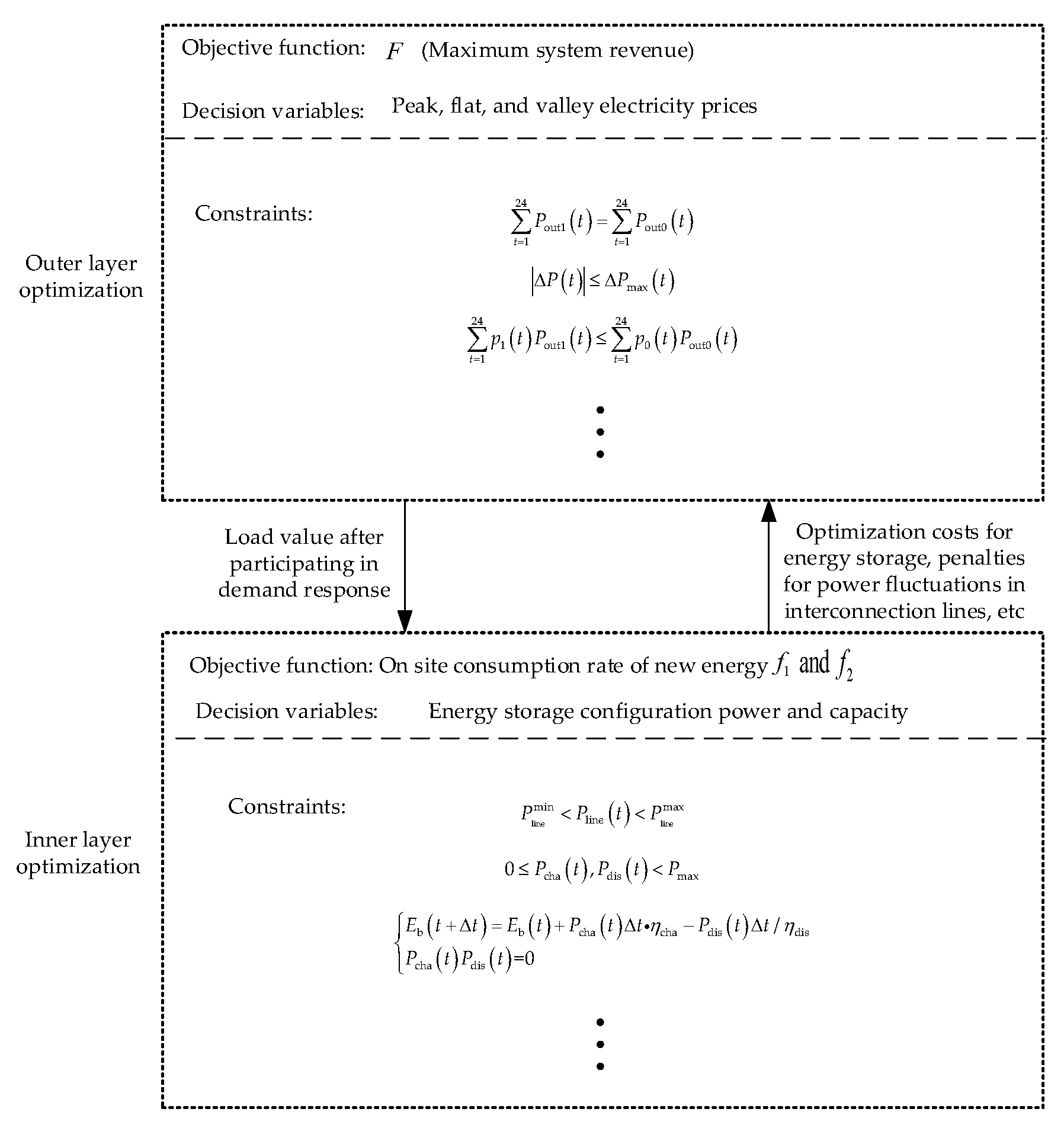
4. Build a Coordinated Optimization Model for Time-of-Use Electricity Prices and Energy Storage Capacity

The user load distribution changes due to demand response, which affects the energy storage configuration and dispatching results of the wind–solar storage system. Different energy storage configurations also affect different time-sharing pricing strategies. In response to the coordination optimization problem of energy storage configuration and dynamic time-of-use electricity price in wind and solar storage systems, this section adopts a double-layer optimization model, with the time-of-use electricity price as the decision variable and the problem of maximizing the revenue of the wind and solar storage system as the objective. The configuration power and capacity of energy storage in the wind and solar storage system are used as the decision variables, and the problem of considering the on-site consumption rate of new energy such as wind and solar and the configuration cost of energy storage is described in the inner layer. The construction architecture of the two-layer optimization model is shown in Figure 2.

4.1. External Revenue Model Considering Demand-Side Response

4.1.1. Objective Function

The outer layer aims to maximize the revenue of the wind and solar energy storage system, which can be expressed as:
max F
In the formula, F represents the revenue of the wind and solar energy storage system. The benefits of the wind and solar energy storage system can be calculated by Equation (11):
F = I sell + I line - grid C grid - line C ope C line + I lc
I sell = t = 1 24 p 1 ( t ) P out 1 ( t ) I line - grid = t = 1 24 p line - grid P line - grid ( t ) C grid - line = t = 1 24 p grid - line P grid - line ( t ) C line = K line 1 24 t = 1 24 P line , t 1 24 t = 1 24 P line , t 2 I lc = t = 1 24 P PV ( t ) + P WT ( t ) r c p c
p 1 t = p g t T g p f t T f p p t T p
In the formula, I sell represents the system’s electricity sales revenue to users; I line - grid represents the revenue from selling electricity to the external power grid of the system; C grid - line represents the cost of purchasing electricity from the solar energy storage system to the external power grid; C ope represents the daily operating cost of energy storage; C line represents the penalty cost for power fluctuations in the interconnection line; I IC represents low-carbon benefits. Carbon trading is a mechanism for reducing carbon dioxide emissions in a market environment, which is an important way to develop a low-carbon economy. Here, low-carbon benefits are quantified and included in the benefits of wind and solar energy storage systems; p 1 t represents the electricity price sold by the optimized wind and solar storage system to users; P out 1 t represents the power after users participate in demand response; P line - grid ( t ) is the selling power of the solar energy storage system to the external power grid, and p line - grid is the purchasing electricity price of the external power grid; P grid - line ( t ) is the purchasing power of the solar energy storage system from the external power grid, and p grid - line is the selling electricity price of the external power grid; P line t and K line respectively represent the power of the interconnection line and its fluctuation penalty coefficient; r c represents the carbon emissions that can be reduced per unit of renewable energy generation, and p c represents the carbon trading price; P WT t and P PV t are the grid power of wind power and photovoltaic power, respectively; p p . p f and p g respectively represent peak, flat, and valley electricity prices; T p , T f , and T g represent peak, flat, and valley periods, respectively.

4.1.2. Constraints

(1)
The total load after the user participates in demand response will remain unchanged, and the load change in any time period will be controlled within a certain range to ensure the power demand of the user.
t = 1 24 P out 1 t = t = 1 24 P out 0 t
Δ P t Δ P max t
(2)
The implementation of time-of-use tariff has changed users’ electricity consumption habits to a certain extent and reduced their comfort. Therefore, it is necessary to ensure the economy of users’ participation in demand response, so as to mobilize users’ enthusiasm for electricity consumption. It is stipulated that the total electricity cost before users’ participation in demand response should not be greater than the total electricity cost when users do not participate in demand response.
t = 1 24 p 1 t P out 1 t t = 1 24 p 0 t P out 0 t
(3)
Improper time-of-use electricity prices can lead to peak–valley inversion or insufficient response, so it is necessary to constrain the peak–valley electricity price ratio.
k 1 p p p g k 2
0 p g < p f < p p p max
In the formula, the range of peak-to-valley electricity price ratio is usually taken as 2–5 [27], and k 1 = 2 and k 2 = 5 are taken; p max is the upper limit of peak electricity price in this paper.
(4)
Marginal cost constraint in valley time
p g C 0
where, C 0 is the marginal cost of the valley period.

4.2. Internal Multi-Objective Model Considering the Daily Life Loss Cost of Energy Storage

Based on the load data optimization results of the outer time-of-use electricity price model, with the goal of maximizing the on-site consumption rate of new energy and minimizing the cost of energy storage configuration, appropriate capacity and power are allocated for the energy storage equipment in the wind and solar storage system. The daily operating cost of the entire life cycle of the energy storage system is further established, and the inner optimization results are fed back to the outer optimization problem for further solving.

4.2.1. Energy Storage Cycle Life Loss Model

In the optimization configuration of energy storage that takes into account the entire life cycle, initial investment cost and cycle life are important factors to consider, while the life loss during energy storage is mainly determined by the discharge depth [28]. Different charging and discharging depths restrict the different recyclable times of energy storage, thereby affecting the length of energy storage cycle life. Among various energy storage materials, lithium batteries have high charging and discharging efficiency as well as high specific energy and power. This article selects lithium battery energy storage as the research object.
(1)
Battery discharge depth
DOD t = 1 SOC t
SOC t = E t E ESS R × 100 %
In the formula, SOC t and DOD t respectively represent the state of charge and discharge depth at time t ; E t is the amount of electricity stored at the time t of energy storage; E ESS R is the rated capacity of energy storage.
(2)
Equivalent number of cycles model
The cycle life of energy storage [29] is shown in (22):
N life = N 0 DOD - k p
In the formula, N life represents the number of cycles in the energy storage life cycle; N 0 represents the number of life cycle cycles corresponding to energy storage at 100% discharge depth; DOD represents the actual discharge depth of energy storage; both N 0 and K p are known parameters given by the energy storage battery manufacturer.
Each time the energy storage battery is charged and discharged, it cannot be guaranteed that the discharge depth remains unchanged. It needs to be converted to a unified standard for statistics. Generally, it is converted according to the equivalent 100% discharge depth. The number of equivalent cycles n eq t for a single time can be calculated using Equation (23):
n eq , t 100 Δ DOD t k p
Δ DOD t = E a t E ESS R
E a t = η cha P cha t + η dis 1 P dis t Δ t
In the formula, η cha and η dis are the charging and discharging efficiency, respectively; P cha t and P dis t are, respectively, charging and discharging power; E a t is the charging and discharging capacity of energy storage during period t ; DOD t represents the discharge depth of energy storage during period t .
The daily equivalent cycle number N eq of energy storage batteries can be obtained from Equation (26):
N eq day = t cha n eq 100 , cha t + t dis n eq 100 , dis t
In the formula, when the energy storage battery is in the charging or discharging state during period t , the equivalent number of cycles during that period is represented by n eq 100 , cha t and n eq 100 , dis t , respectively.
(3)
The equivalent cycle life of energy storage is
T cyc = N 0 365 · N eq day
(4)
The daily cycle life loss cost of energy storage is
C loss = c P P ESS R + c E E ESS R β 1 + β T cyc 365 · 1 + β T cyc 1
K ESS D = β 1 + β T cyc 365 · 1 + β T cyc 1
In the formula, c P and c E are the cost per unit power and per unit capacity of the energy storage system, respectively; β is the discount rate; K ESS D is the isodiurnal coefficient; E ESS R and P ESS R represent the rated capacity and power of the energy storage configuration, and they are the internal decision variables.

4.2.2. Daily Cost of Energy Storage throughout Its Entire Life Cycle

The daily operating cost C ope of the entire life cycle of the energy storage system is composed of the daily investment cost C investment , daily operation and maintenance cost C maintenance , and daily loss cost C loss . The calculation formula is shown in Equation (32).
C investment = c P P ESS R + c E E ESS R β 1 + β Y a 365 × 1 + β Y a 1
C maint = c maint E ESS R 365
C ope = C investment + C maintenance + C loss
In the formula, Y a is the investment period of the energy storage system; C m a int is the average annual maintenance cost per unit capacity of energy storage.

4.2.3. Objective Function

In the formula, f 1 is the on-site consumption rate of new energy; f 2 is the configuration cost of energy storage, P SC t . P bat t represents the new energy consumed by the load and energy storage at time t .
max   f 1 f 1 = t = 1 24 P SC t + P bat t t = 1 24 P PV t + P WT t × 100 % , P SC t = min P PV t + P WT t , P out t min f 2 f 2 = c E × E ESS R + c P × P ESS R

4.2.4. Constraints

(1)
Power balance constraints
P WT t + P PV t + P ESS t P line t = P load t 0 P WT t P WTY t 0 P PV t P PVY t 0 P load t P loadX t P loss t = P loadX t P load t P waste t = P WTY t + P PVY t P WT t P PV t
In the formula, P WT t and P PV t are the actual grid power of wind power and photovoltaic power during time t , respectively; P load t is the actual load power supplied by the system during period t ; P WTY t and P PVY t are the predicted power of wind power and photovoltaic power during the t period, respectively; P loadX t is the load power transmitted from the outer layer to the inner layer during the t period; P ESS t is the energy storage charging and discharging power during period t ; P loss t is the power loss during period t ; P waste t represents the excess power of wind and solar power during the t period.
(2)
Transmission power constraints of interconnection lines
P line min < P line t < P line max
In the formula, P line max and P line min are the upper and lower limits of the transmission power of the interconnection line, respectively.
(3)
Energy storage operation constraints
During any period of time, the charging and discharging power of the energy storage system is limited to
0 P cha t , P dis t < P max
In the formula, P cha t and P dis t respectively represent the charging and discharging power during the energy storage period t , and P max represents the maximum charging and discharging power.
E b t + Δ t = E b t + P cha t Δ t × η cha P dis t Δ t / η dis P cha t P dis t = 0
In the formula, E b t is the energy storage capacity at time t . To avoid overcharging and discharging of energy storage, then
SOC t = E b t E ESS R SOC min < SOC t < SOC max
In the equation, SOC max and SOC min are the maximum and minimum values of SOC .
To ensure the sustainability of the scheduling cycle of the energy storage system, the state of charge is consistent throughout a cycle, i.e.,
SOC 0 = SOC 24
(4)
Limited by factors such as investment funds and site conditions, the power and capacity of energy storage are constrained
P ESS min < P ESS R < P ESS max
E ESS min < E ESS R < E ESS max
In the formula, P ESS max , P ESS min , E ESS max , and E ESS min are the boundary values of the configured power and capacity of the energy storage system allowed by the installation conditions.

4.2.5. Optimal Scheduling Strategy for Wind and Solar Energy Storage Systems

In the operation of the wind and solar storage grid-connected system, a strategy of joint interaction between the energy storage system and the external power grid is adopted to balance the output of new energy such as wind and solar in the system and the electricity demand of users. The optimization control strategy proposed in this article is shown in Appendix A Figure A1. P net is the net load, that is, P net = P load P PV P WT , which detects the difference between P net and the energy storage system SOC , and determines the magnitude of t period P net t and the rated power P ESS R of the energy storage system, then adjusts accordingly to balance the main body of the fluctuation in wind and solar energy storage power. When P net t is greater than P ESS R , the external power grid is mainly used to supply the power demand of the load, and the portion exceeding the power limit of the tie line is supplied by the energy storage system for the load. If P net t is within the power supply capacity of the interconnection line, the external power grid should consider charging the energy storage system while supplying electricity; When P net t is less than zero or greater than zero and less than P ESS R , this situation mainly relies on the energy storage system to maintain the balance of P net t . If P net t is less than zero, first consider charging the energy storage system, then consider selling the remaining electricity to the external power grid. If P net t is less than zero, the energy storage system is first considered to be charged, and the remaining electricity is considered to be sold to the external power grid. If P net t is greater than zero and less than P ESS R , priority will be given to discharging the energy storage system, and for the part with insufficient electricity, external grid electricity will be purchased. In the entire control strategy, the charging and discharging of energy storage should be dynamically adjusted based on the SOC state to avoid the problem of energy storage system SOC exceeding the limit. When SOC t 1 is in the boundary state SOC min , the energy storage system does not perform discharge operation, and when SOC t 1 is in the boundary state SOC max , the energy storage system does not perform charging operation. If the energy storage system exceeds the boundary state P cha t or P dis t after charging and discharging with SOC min or SOC max , the charging and discharging power needs to be corrected according to Equations (42) and (43).
P cha t = S O C max S O C t 1 η cha E ESS R
P dis t = S O C t 1 S O C min E ESS R η dis

5. Model Solving Algorithms and Processes

5.1. Solution Algorithm

The model solving algorithms in this article include the improved sparrow algorithm and the multi-objective particle swarm optimization algorithm, among which the ISSA algorithm can refer to reference [30,31]. The basic concepts of multi-objective particle swarm algorithm are as follows.

5.1.1. Multi-Objective Particle Swarm Optimization Algorithm

The multi-objective particle swarm optimization algorithm, like the sparrow algorithm, is also a biomimetic algorithm where individuals in the population participate in cooperation and competition using a velocity displacement model to guide optimization searches. The evolutionary process is as follows:
v i , j k + 1 = w × v i , j k + c 1 r 1 × p i , j k x i , j k + c 2 r 2 × g i , j k x i , j k , j = 1 , 2 , n x i , j k + 1 = x i , j k + v i , j k + 1 w = w max w max w min × k K max
In the formula, n is the number of individuals in the population; w is the inertia weight used for manipulating algorithm development and exploration scales, K max is the number of iterations, w max , w min are artificially set empirical values, and k is the current algebra; c 1 , c 2 is the learning factor; r 1 and r 2 are random numbers within 0 , 1 ; v i , j k and x i , j k correspond to the individual’s position and speed respectively; p i , j k and g i , j k are individual extreme value and global extreme value determined by fitness function respectively.
The above internal function Equation (33) can be summarized as the following multi-objective model:
max f E , P min R E , P   s · t ·   g E , P = 0   h E , P 0
In the formula, F E , P and R E , P are the objective functions of the on-site consumption rate of new energy and the purchase cost of energy storage, respectively; g E , P and h E , P represent equality and inequality constraints, respectively; E and P represent the configured capacity and configured power of energy storage.
For F E , P and R E , P , the two objective functions interact and constrain each other, making it difficult for them to achieve optimal results simultaneously. Instead, they are replaced by the Pareto optimal solution [32,33]. These solutions are mapped by functions F E , P and R E , P to form the optimal frontier of Pareto . The solution to Equation (45) is to find a sufficient number of optimal solutions for Pareto and try to distribute the optimal frontier diagram evenly, in order to provide reference for power practitioners.

5.1.2. Choosing the Compromise Optimal Solution

After obtaining the Pareto optimal solution set, the optimal compromise solution is determined using fuzzy mathematics [34]. Using fuzzy membership functions to characterize the satisfaction of the solution set elements corresponding to various dimensional functions:
μ i m = 1       f i m f m , min f m , max f i m f m , max f m , min , f m , min < f i m < f m , max 0       f i m f m , max
In the equation, f i m is the objective function, m 1 , 2 , , N o b j ; f m , max and f m , min are the maximum and minimum values corresponding to f i m , respectively.
The satisfaction calculation of each Pareto optimal solution is shown in Equation (47), and the corresponding solution when it reaches its maximum is considered the optimal compromise solution.
μ i = m = 1 N obj μ i m i = 1 N c m = 1 N obj μ i m
In the equation, N c is the number of Pareto optimal solutions.

5.2. Energy Storage Charging and Discharging Verification

Inner-layer optimization belongs to the multi-time period coupling optimization problem, which means that the operating state of energy storage is not only constrained by its capacity and maximum charging and discharging power but also related to multiple other time periods. The constraint of equal starting and ending energy during the daily operation cycle of energy storage, as shown in Equation (38), is not easy to implement. To this end, a backstepping method is proposed to verify and adjust the capacity status of each period of energy storage, as follows:
(1)
First, based on the decision variables of energy storage capacity and maximum charging and discharging power at the lower level, and on the principle that the initial state of charge SOC ( 0 ) of energy storage is equal to the end time SOC ( 24 ) , the maximum state of charge SOC t max and minimum state of charge SOC t min that should be constrained for each time period SOC ( 23 ) , SOC ( 22 ) ... SOC ( t ) are derived.
SOC t max = min 0.5 + 24 t · P d R / η d · E ess R , 0.9
SOC t min = max 0.5 24 t · η c · P c R / E ess R , 0.2
(2)
Detect and correct P c t and P d t
P d t = min x , SOC t 1 SOC t min · η d · E ess R s · t ·   SOC t < SOC t min P c t = max x , SOC t 1 SOC t max · E ess R / η c s · t ·   SOC t > SOC t max
In the formula, x represents other constraints that need to be comprehensively considered during the energy storage charging and discharging process.
(3)
Detect and correct P c t + 1 and P d t + 1 based on, SOC t + 1 max , SOC t + 1 min , until SOC ( 24 ) equal SOC ( 0 ) .

5.3. Solution Flowchart

The improved sparrow algorithm is used to solve the outer layer of the model to optimize electricity price. Users actively respond to the electricity price policy and transfer the load after participating in demand response to the inner layer. The inner layer uses the common multi-objective particle swarm optimization algorithm to solve the problem. The objective function is to coordinate and optimize the capacity and maximum charging and discharging power of the energy storage system, taking the on-site consumption rate of new energy and the optimization configuration cost of energy storage as the objective functions. The optimization results are fed back to the outer layer to participate in the optimization of the outer layer decision variables. The solving process of the double-layer multi-objective model is shown in Appendix A Figure A2.

6. Example Analysis

6.1. Example Parameter Description

To verify the rationality of the model proposed in this article, a simplified wind and solar energy storage grid-connected system is used as an example to study the optimization configuration of energy storage capacity. The relevant parameters are shown in Table 1.
Wind power, photovoltaic power, and load are all selected according to the typical daily power curve according to the season. Due to the close relationship between wind, light, and load power curves in spring and autumn, the situation in autumn is not considered, and spring is referred to as the transitional season, as shown in Appendix A Figure A3. The initial electricity price is shown in Table 2.
Based on the example data combined with the mathematical model described earlier, the solution algorithm can be used to optimize the model. The subsequent analysis of the results will mainly optimize the expressions based on the three objective functions mentioned in the previous text, namely Equations (2), (11) and (33). The division of time periods for dynamic time-of-use electricity prices mainly relies on functional Equation (2). The calculation of the electricity price value, energy storage power and capacity, on-site consumption rate of wind and solar energy, and economic cost of wind and solar energy storage systems for dynamic time-of-use electricity prices is mainly based on the final optimization solution results of outer objective Equation (11) and inner optimization objective Equation (33).

6.2. Optimization Configuration Results under Different Typical Weather Conditions

Due to the different distribution characteristics of net load in different seasons and time periods, it is necessary to divide the peak-to-valley electricity prices into three scenarios, as shown in Figure 3. From the figure, it can be seen that the electricity prices under three typical daily scenarios are different in size and distribution during peak-to-valley periods. Taking peak electricity prices as an example, the highest electricity price is in summer, with a peak value of 0.91 RMB/kW·h, and the peak electricity prices in transition season and winter are 0.75 RMB/kW·h and 0.73 RMB/kW·h, respectively.
Figure 4 and Table 3 show the optimization solution results under different seasonal scenarios. From this, it can be concluded that the energy storage capacity configuration scale in summer is the largest, reaching 1194 kW·h, and the energy storage configuration power in spring is the largest, reaching 210 kW. When configuring the energy storage capacity of the system, the energy storage configuration results of the typical day with the highest demand are considered the energy storage planning standard of the system. Therefore, based on the energy storage configuration results of three typical scenarios, the final energy storage scale configured in this combined power generation system is 1194 kW·h capacity and 210 kW power.
To study the coordination relationship between energy storage configuration and electricity price in wind and solar energy storage systems, typical summer days are selected as the energy storage configuration carriers, and the following scenarios are set up for further comparative analysis:
Scenario 1: Revenue from wind and solar systems (excluding energy storage) and on-site consumption of new energy without implementing dynamic time-of-use electricity prices.
Scenario 2: Implementation of dynamic time-of-use electricity prices for wind and solar systems (excluding energy storage) and on-site consumption of new energy.
Scenario 3: Revenue and internal multi-objective optimization of wind and solar energy storage systems without implementing dynamic time-of-use pricing.
Scenario 4: Implementing the revenue and internal multi-objective optimization of wind and solar energy storage systems under dynamic time-of-use electricity prices.

6.3. Analysis of Simulation Results

6.3.1. Analysis of On-Site Consumption of New Energy

Table 4 shows the results of energy storage configuration scale and on-site consumption rate under four different scenarios. From Table 4, it can be seen that compared to Scenario 1, the on-site consumption rate of new energy in Scenario 2 has increased by 4.12%, indicating that implementing the time-of-use electricity price can improve the distribution characteristics of the initial predicted load and enhance the absorption capacity of the wind and solar storage system for new energy. Compared with Scenario 1, the on-site consumption rate of new energy in Scenario 3 has increased by 2.34%, indicating that the system is equipped with energy storage facilities to store excess local wind and solar resources, thereby reducing the electricity output of new energy from the wind and solar storage system to the external power grid. Scenario 4 has the highest on-site consumption rate of new energy, as the optimized time-of-use electricity price through the outer layer provides the inner layer with a load that has undergone demand-side response. The peak–valley difference and volatility of the load curve are reduced, and the flexible adjustment ability of the system’s new energy is further improved through the charging and discharging actions of energy storage in the inner layer. Figure 5 depicts the relationship between the energy storage configuration and the on-site consumption rate of new energy in Scenarios 3 and 4. It can be seen from the figure that when the wind and solar storage system achieves the same on-site consumption rate of new energy, Scenario 3 needs to be configured with a larger energy storage capacity. This further demonstrates that the optimized time-of-use electricity price is conducive to further improving the on-site consumption rate of new energy.
Table 5 and Figure 6 show the characteristic changes in typical daily load in summer before and after participating in demand response. From Table 5 and Figure 6, it can be concluded that users have a high demand for electricity from 11:00–14:00 and from 18:00–21:00, with insufficient wind and photovoltaic output and net load in the peak range. Therefore, these periods are divided into peak periods. Users consume less electricity during the period from 1:00 to 8:00, wind power has a higher output during this period, and the net load takes a smaller value during the day. This period is divided into valley periods, and the rest of the period is divided into regular periods. According to the net load, the peak-to-valley electricity price periods are further optimized, and the optimized electricity prices for valley, flat, and peak periods are 0.28 RMB/kW·h, 0.42 RMB/kW·h, and 0.91 RMB/kW·h, respectively. The optimized load curve reduces the peak–valley difference, the peak load decreases by 17.3 kW, and the valley load increases by 88.4 kW. From the calculation results and Figure 6, it can be seen that the demand response strategy can effectively stabilize the load peak–valley difference and the net load peak–valley difference. The total load before users’ participation in demand response remains unchanged, and Table 4 shows that the total price before users’ participation is 14,301 RMB, and the total price after response is 13,238 RMB, which meets the constraint setting requirements of demand response in the model, and the reduced power cost helps to improve the enthusiasm and feasibility of users’ participation in demand response.
Figure 7 shows optimization scheduling results under four different scenarios. Figure 8 shows the energy storage charging and discharging power and charging state of each period in Scenario 3 and Scenario 4. The initial charging state of the energy storage is 0.5, and it recovers to 0.5 at the end of one cycle, meeting the sustainability of the energy storage system scheduling cycle. According to the scheduling strategy mentioned earlier, the non-on-site consumption period of new energy is distributed during the period when the wind and solar output exceeds the load demand. From Figure 7a, it can be seen that the non-on-site consumption period of new energy is from 1:00 to 8:00, as well as at 22:00 and 24:00. From Figure 7b, it can be seen that the user load after demand response increases at these moments, thus reducing the surplus of the scenery. As shown in Figure 7c,d, when energy storage devices are installed in the new energy system, energy storage will absorb a portion of excess wind and solar new energy during the remaining hours of 1:00–3:00 and 22:00, thereby improving the on-site consumption rate of new energy.

6.3.2. Economic Analysis

Table 6 shows the system benefits under four scenarios. Compared with Scenario 2, Scenario 1 has an increase of 1560 RMB in system revenue. As users participate in the demand response policy, the revenue from selling electricity to users in the system has decreased by 1063 RMB, but in Scenario 2, the penalty for contact line fluctuation has decreased by 2519.6 RMB, and in Scenario 2, the system revenue has increased. Although there is a small difference between Scenario 1 and Scenario 2 and the settlement amount of purchasing and selling electricity from the external network, the scale of single purchasing and selling electricity in Scenario 1 is larger than that in Scenario 2. This also verifies the conclusion that demand response policy can improve the local consumption rate of new energy. Compared with Scenario 1, Scenario 3 showed a decrease of 3307.6 RMB in system revenue. This difference is mainly due to the daily loss cost of energy storage equipment in the system and the penalty for contact line fluctuations. As a result, the reduction in electricity purchase revenue from the grid also indicates that Scenario 3 with energy storage facilities has improved the on-site consumption rate of new energy compared to Scenario 1 without energy storage facilities. Compared with Scenarios 1 and 3, Scenario 4 has the highest system revenue, mainly due to the significant reduction in penalties for tie line fluctuations. This indicates that the method proposed in this article can better suppress power fluctuations in the interconnection line. This method has the lowest electricity sales revenue for the power grid, which minimizes the sales of new energy to external power grids. This reduces the impact of integration fluctuations between new energy and external power grids in wind and solar energy storage systems, and improves the safe and stable operation of the power grid. Compared with Scenario 2, the decrease in system revenue in this scenario mainly comes from the daily loss cost of energy storage, but the on-site consumption of new energy in Scenario 4 is better than that in Scenario 2.

6.3.3. Optimization Results of Different Penalty Factors

To study the impact of power fluctuation penalties on interconnection lines, three different penalty values, 0.1, 0.01, and 0.001, are set. The solution results under different scenarios are shown in Table 7. From the table, it can be seen that in scenarios 1 to 4, for each scenario with the same on-site consumption rate and energy storage configuration scale of new energy, the system revenue is maximum at a penalty factor of 0.001, and minimum at a penalty factor of 0.1.
The inner model is solved under the set control strategy. When the load transmitted from the outer layer to the inner layer is the same and the energy storage configuration scale of the inner layer is the same, the variables in the inner layer of the model obtain the same results, The main change at this point comes from the power fluctuation penalty of the interconnection line. When the penalty coefficient is large, the system revenue will correspondingly decrease. Under the penalty factors of 0.001 and 0.01, the revenue in Scenario 1 is the largest, and the revenue in Scenario 4 is the smallest. This indicates that some users participate in demand response, reducing the revenue of the system, and the system configured with energy storage also increases the energy storage loss, which is greater than the loss caused by the system reducing the power fluctuation of the tie line. When the penalty factor is 0.1, the fluctuation penalty cost of Scenario 1 and Scenario 2 is relatively large, which greatly reduces system revenue. At this time, Scenario 4 has the largest system revenue, because this scenario has the smallest power fluctuation of tie lines under the influence of demand response and energy storage configuration.

7. Conclusions

This article studies the allocation of energy storage capacity considering electricity prices and on-site consumption of new energy in wind and solar energy storage systems. A nested two-layer optimization model is constructed, and the following conclusions are drawn:
(1) The distribution of source load power curves varies for typical days in different seasons. Using dynamic time-of-use electricity prices can more flexibly obtain the capacity configuration scale of energy storage. The article adopts the capacity and maximum power values of energy storage configuration in each season, which can meet the demand for energy storage capacity in each season. The optimization of park electricity prices can slightly increase the on-site consumption rate of new energy, while energy storage can significantly increase the consumption rate of new energy, but the cost of energy storage configuration is relatively high. This article proposes a coordinated optimization method for energy storage and electricity prices in the park, which can achieve maximum on-site consumption of new energy while improving the economy of energy storage to a certain extent.
(2) This article adopts a joint optimization model of load demand-side response and energy storage configuration, which can effectively improve the revenue of wind and solar storage systems and the on-site consumption rate of new energy, and greatly reduce the fluctuation penalty of connecting lines.
(3) The energy storage daily loss model proposed in this article can accurately reflect the operational loss of energy storage, and the proposed backstepping method can effectively verify and adjust the capacity status of each period of energy storage, ensuring that the optimization of energy storage has equal states of charge from beginning to end.
(4) This article does not consider user satisfaction factors and does not analyze the impact of typical day prediction errors on energy storage configuration results when participating in demand-side response. The next step can focus on this point.

Author Contributions

Conceptualization, W.H. and X.Z.; methodology, W.H. and X.Z.; software, L.Z.; validation, W.H. and Z.L. All authors have read and agreed to the published version of the manuscript.

Funding

This research was funded by the Natural Science Foundation of Xinjiang Uygur Autonomous Region (2021D01C044).

Data Availability Statement

All data and materials generated or analysed during this study are included in this published article.

Conflicts of Interest

There are no conflict of interest to declare.

Appendix A

Figure A1. Optimization operation strategy for wind and solar storage system.
Processes 11 01725 g0a1
Figure A2. Double layered multi-objective optimization calculation process.
Processes 11 01725 g0a2
Figure A3. Predicted values of solar and load power before the day.
Processes 11 01725 g0a3

References

  1. Koohi-Fayegh, S.; Rosen, M.A. A review of energy storage types, applications and recent developments. J. Energy Storage 2020, 27, 101047. [Google Scholar] [CrossRef]
  2. Beshir, M.J.; Farag, A.S.; Cheng, T.C. New comprehensive reliability assessment framework for power systems. Energy Convers. Manag. 1999, 40, 975–1007. [Google Scholar] [CrossRef]
  3. Tushar, M.H.K.; Zeineddine, A.W.; Assi, C. Demand-side management by regulating charging and discharging of the ev, ess, and utilizing renewable energy. IEEE Trans. Ind. Inform. 2018, 14, 117–126. [Google Scholar] [CrossRef]
  4. Snoussi, J.; Elghali, S.B.; Benbouzid, M.; Mimouni, M.F. Optimal sizing of energy storage systems using frequency-separation-based energy management for fuel cell hybrid electric vehicles. IEEE Trans. Veh. Technol. 2018, 67, 9337–9346. [Google Scholar] [CrossRef]
  5. Khezri, R.; Mahmoudi, A.; Haque, M.H. Impact of optimal sizing of wind turbine and battery energy storage for a grid-connected household with/without an electric vehicle. IEEE Trans. Ind. Inform. 2022, 18, 5838–5848. [Google Scholar] [CrossRef]
  6. Li, F.; Li, X.; Zhang, B.; Li, Z.; Lu, M. Multiobjective optimization configuration of a prosumer’s energy storage system based on an improved fast nondominated sorting genetic algorithm. IEEE Access 2021, 9, 27015–27025. [Google Scholar] [CrossRef]
  7. Khezri, R.; Mahmoudi, A.; Haque, M.H. Optimal capacity of solar pv and battery storage for australian grid-connected households. IEEE Trans. Ind. Appl. 2020, 56, 5319–5329. [Google Scholar] [CrossRef]
  8. Wu, J.; Ding, M.; Zhang, J. Capacity configuration method of energy storage system for wind farm based on cloud model and k-means clustering. Automat. Electron. Power Syst. 2018, 42, 67–73. [Google Scholar]
  9. El-Bidairi, K.S.; Duc Nguyen, H.; Jayasinghe, S.D.G.; Mahmoud, T.S.; Penesis, I. A hybrid energy management and battery size optimization for standalone microgrids: A case study for flinders island, australia. Energy Convers. Manag. 2018, 175, 192–212. [Google Scholar] [CrossRef]
  10. Kong, X.; Wang, H.; Li, N.; Mu, H. Multi-objective optimal allocation and performance evaluation for energy storage in energy systems. Energy 2022, 253, 124061. [Google Scholar] [CrossRef]
  11. Cai, J.; Xu, Q.; Yuan, X.; Wang, X. Configuration strategy of large-scale battery storage system orienting wind power consumption based on temporal scenarios. High Volt. Eng. 2019, 45, 993–1001. [Google Scholar]
  12. Barrera-Santana, J.; Sioshansi, R. An optimization framework for capacity planning of island electricity systems. Renew. Sustain. Energy Rev. 2023, 171, 112955. [Google Scholar] [CrossRef]
  13. Naderipour, A.; Ramtin, A.R.; Abdullah, A.; Marzbali, M.H.; Nowdeh, S.A.; Kamyab, H. Hybrid energy system optimization with battery storage for remote area application considering loss of energy probability and economic analysis. Energy 2022, 239, 122303. [Google Scholar] [CrossRef]
  14. Nazir, M.S.; Abdalla, A.N.; Wang, Y.; Chu, Z.; Jie, J.; Tian, P.; Jiang, M.; Khan, I.; Sanjeevikumar, P.; Tang, Y. Optimization configuration of energy storage capacity based on the microgrid reliable output power. J. Energy Storage 2020, 32, 101866. [Google Scholar] [CrossRef]
  15. Pires, A.L.G.; Rotella Junior, P.; Rocha, L.C.S.; Peruchi, R.S.; Janda, K.; Miranda, R.D.C. Environmental and financial multi-objective optimization: Hybrid wind-photovoltaic generation with battery energy storage systems. J. Energy Storage 2023, 66, 107425. [Google Scholar] [CrossRef]
  16. Premadasa, P.N.D.; Silva, C.M.M.R.; Chandima, D.P.; Karunadasa, J.P. A multi-objective optimization model for sizing an off-grid hybrid energy microgrid with optimal dispatching of a diesel generator. J. Energy Storage 2023, 68, 107621. [Google Scholar] [CrossRef]
  17. Kou, L.; Ji, Y.; Wu, M.; Niu, G. Optimal configuration of multi-energy complementary system considering full life cycle. Electric Power 2020, 53, 75–82. [Google Scholar]
  18. Yan, N.; Zhang, B.; Li, W.; Ma, S. Hybrid energy storage capacity allocation method for active distribution network considering demand side response. IEEE Trans. Appl. Supercond. 2019, 29, 1–4. [Google Scholar] [CrossRef]
  19. Murty, V.V.S.N.; Kumar, A. Optimal energy management and techno-economic analysis in microgrid with hybrid renewable energy sources. J. Mod. Power Syst. Clean Energy 2020, 8, 929–940. [Google Scholar] [CrossRef]
  20. Honarmand, H.A.; Rashid, S.M. A sustainable framework for long-term planning of the smart energy hub in the presence of renewable energy sources, energy storage systems and demand response program. J. Energy Storage 2022, 52, 105009. [Google Scholar] [CrossRef]
  21. Kiptoo, M.K.; Lotfy, M.E.; Adewuyi, O.B.; Conteh, A.; Howlader, A.M.; Senjyu, T. Integrated approach for optimal techno-economic planning for high renewable energy-based isolated microgrid considering cost of energy storage and demand response strategies. Energy Convers. Manag. 2020, 215, 112917. [Google Scholar] [CrossRef]
  22. Mohseni, S.; Brent, A.C.; Kelly, S.; Browne, W.N.; Burmester, D. Strategic design optimisation of multi-energy-storage-technology micro-grids considering a two-stage game-theoretic market for demand response aggregation. Appl. Energy 2021, 287, 116563. [Google Scholar] [CrossRef]
  23. Zhu, C.; Lu, W.; Zhao, W.; Hong, Z.; Chen, C. On-site energy consumption technologies and prosumer marketing for distributed poverty alleviation photovoltaic linked to agricultural loads in china. IEEE Access 2020, 8, 191561–191573. [Google Scholar] [CrossRef]
  24. Sun, Y.; Cui, C.; Lu, J.; Hao, J.; Liu, X. Non-intrusive load monitoring method based on delta feature extraction and fuzzy clustering. Automat. Electron. Power Syst. 2017, 41, 86–91. [Google Scholar]
  25. Karapetyan, A.; Khonji, M.; Chau, S.C.; Elbassioni, K.; Zeineldin, H.; El-Fouly, T.H.M.; Al-Durra, A. A competitive scheduling algorithm for online demand response in islanded microgrids. IEEE Trans. Power Syst. 2021, 36, 3430–3440. [Google Scholar] [CrossRef]
  26. Muthirayan, D.; Kalathil, D.; Poolla, K.; Varaiya, P. Mechanism design for demand response programs. IEEE Trans. Smart Grid 2020, 11, 61–73. [Google Scholar] [CrossRef] [Green Version]
  27. Li, C.; Xu, Z.; Ma, Z. Optimal time-of-use electricity price model considering customer demand response. Proc. CSU-EPSA 2015, 27, 11–16. [Google Scholar]
  28. Wang, K.; Qiao, Y.; Xie, L.; Li, J.; Lu, Z.; Yang, H. A fuzzy hierarchical strategy for improving frequency regulation of battery energy storage system. J. Mod. Power Syst. Clean Energy 2021, 9, 689–698. [Google Scholar] [CrossRef]
  29. Tran, D.; Khambadkone, A.M. Energy management for lifetime extension of energy storage system in micro-grid applications. IEEE Trans. Smart Grid 2013, 4, 1289–1296. [Google Scholar] [CrossRef]
  30. Zhu, L.; Hu, W. Short term wind speed prediction based on vmd and dbn combined model optimized by improved sparrow intelligent algorithm. IEEE Access 2022, 10, 92259–92272. [Google Scholar] [CrossRef]
  31. Zhang, C.; Ding, S. A stochastic configuration network based on chaotic sparrow search algorithm. Knowl. -Based Syst. 2021, 220, 106924. [Google Scholar] [CrossRef]
  32. Cui, Y.F.; Geng, Z.Q.; Zhu, Q.X.; Han, Y.M. Review: Multi-objective optimization methods and application in energy saving. Energy 2017, 125, 681–704. [Google Scholar] [CrossRef]
  33. Qu, B.; Li, C.; Liang, J.; Yan, L.; Yu, K.; Zhu, Y. A self-organized speciation based multi-objective particle swarm optimizer for multimodal multi-objective problems. Appl. Soft Comput. 2020, 86, 105886. [Google Scholar] [CrossRef]
  34. Fei, Z.S.; Li, B.; Yang, S.S.; Xing, C.W.; Chen, H.B.; Hanzo, L. A survey of multi-objective optimization in wireless sensor networks: Metrics, algorithms, and open problems. IEEE Commun. Surv. Tutor. 2017, 19, 550–586. [Google Scholar] [CrossRef] [Green Version]
Figure 1. Wind and solar storage system.
Processes 11 01725 g001
Figure 2. Architecture of the bilevel programming model.
Processes 11 01725 g002
Figure 3. Optimization results of time-of-use electricity prices in different seasons.
Processes 11 01725 g003
Figure 4. Configuration of energy storage in different seasons.
Processes 11 01725 g004
Figure 5. Configuration of energy storage before and after demand response.
Processes 11 01725 g005
Figure 6. Summer electricity price optimization and source load changes.
Processes 11 01725 g006
Figure 7. Optimization scheduling results for four scenarios.
Processes 11 01725 g007
Figure 8. Energy storage charge and discharge power and state of charge for Scenarios 3 and 4.
Processes 11 01725 g008
Table 1. Simulation parametersis.
ParameterNumerical ValueParameterNumerical Value
Penalty cost coefficient0.1Cross elasticity coefficient0.03
Ciscounted rate5%cp (RMB/kW) 1085
Kp2 P line max (kW)600
Maximum number of charges and disCharges for energy storage5000 P line min (kW)−600
Carbon trading price (RMB/1000 kg)15cE (RMB/kW) 3224
η c , η d 0.95Operation and maintenance Costs (RMB/kW h)50
SOC max 0.9 E ESS max 2500
SOC min 0.2 P ESS max 500
SOC initial value0.5Carbon reduction per unit of New energy (kg/kW·h)0.16
Electricity selling price0.58 C 0 (RMB/kW·h)0.12
Electricity purchase price0.69 p max (RMB/kW·h)1.2
Coefficient of self elasticity−0.2 Y a /Year20
Table 2. Initial time-of-use tariff table.
ParameterPeriod of TimeElectricity Price (RMB/kW·h)
Peak period07:00–11:00, 17:00–21:000.96
Peacetime period12:00–16:00, 22:00–23:000.58
Valley period00:00–6:000.27
Table 3. Optimization results of typical days in three seasons.
Typical Daily ScenarioOn Site Consumption Rate of New Energy Energy   Storage   Capacity / ( kW · h ) Energy   Storage   Power / ( kW )
Peak period07:00–11:00, 17:00–21:00285210
Peacetime period12:00–16:00, 22:00–23:001194136
Valley period00:00–6:00826192
Table 4. Optimization results of typical days in three Seasons.
SceneOn Site Consumption Rate of New Energy/% Energy   Storage   Capacity / ( kW · h ) Energy   Storage   Power / ( kW )
191.55%00
295.67%00
393.89%1194210
497.93%1194210
Table 5. Demand response effect.
Before and after OptimizationMaximum Load/kWMinimum Load/kWPeak–Valley Difference of Load/kWNet Load Peak Valley Difference/kW
Before optimization1356.3458.6897.7646.9
After optimization1339547792411.4
Variation−17.388.4−105.7−235.5
Table 6. Economic analysis under different scenarios (Unit:RMB).
SceneSystem BenefitsConsumer Electricity ConsumptionRevenue from Selling Electricity to the Power GridCost of Purchasing Electricity from the Power GridPenalty for Contact Line FluctuationsDaily Loss Cost of Energy Storage
110,35414,3011124.91514.93612.10
211,91413,238576.17863.191092.50
37046.414,301985.511426.35197.71670.9
410,52713,238276.12560.53856.431625.7
Table 7. EffectSystem returns and contact line fluctuation penalties under different penalty factors.
Different ScenariosReturns and Volatility PenaltiesDifferent Penalty Factors
0.10.010.001
Scenario 1System benefits10,35413,60513,930
Volatility Penalties3612.1361.2136.12
Scenario 2System benefits11,91412,89712,995
Volatility Penalties1092.5109.2510.93
Scenario 3System benefits7046.411,72512,192
Volatility Penalties5197.7519.7751.98
Scenario 4System benefits10,52711,29711,374
Volatility Penalties856.4385.648.56
Disclaimer/Publisher’s Note: The statements, opinions and data contained in all publications are solely those of the individual author(s) and contributor(s) and not of MDPI and/or the editor(s). MDPI and/or the editor(s) disclaim responsibility for any injury to people or property resulting from any ideas, methods, instructions or products referred to in the content.

