CFD Modeling of Phase Change during the Flashing-Induced Instability in a Natural Circulation Circuit

Abstract

Flashing-induced instability (FII) has a significant impact on the safe operation of a natural circulation circuit, a phenomenon frequently encountered in the cooling systems of advanced light water reactors. While one-dimensional system codes are commonly used for the engineering design and safety analysis of FII, there is a strong academic interest in understanding the underlying physical mechanisms. To address this, high-resolution computational fluid dynamics (CFD) simulations serve as a valuable tool. However, the current state of CFD modeling for two-phase flows with phase change, which are particularly highly transient fluctuating flashing flows, is still in its early stages of development. In this study, we establish a CFD model that focuses on interphase heat transfer to analyze the phase change during FII. By incorporating experimental data from the literature, we investigate the transient flow field and thermodynamic behavior in the riser of the GENEVA test facility. The study provides valuable insights into the non-equilibrium and interfacial transfer phenomena during the phase change as well as the effect of high-frequency fluctuation. Additionally, we discuss in detail the challenges associated with FII modeling and the limitations of the current model. We also provide suggestions for potential improvements in future numerical studies. The results show that the thermal phase change and heat transfer coefficient model adopted for the simulation reasonably captures the evaporation and condensation process. However, it tends to under-predict the evaporation rate, which results in a larger pressure drop through the riser. The observation that the void fraction close to the wall is higher than that in the riser center evidences that the reliable modeling of bubble size distribution as well as the inclusion of non-drag forces are important for predicting the transverse void distribution. Furthermore, it reveals that both the temperature and pressure change in an FII, and their effects on phase change should be taken into account simultaneously.

1. Introduction

The term of flashing (or flash evaporation, flash boiling) refers to the phase change phenomenon in which an initially subcooled liquid is superheated and vaporized due to pressure drop under nearly adiabatic boundary conditions. In practice, it can occur when the area of a flow channel reduces, e.g., through a nozzle, and the flow accelerates; the pressure of the fluid system decreases due to cracks or other openings, or the hydrostatic pressure decreases as the elevation increases [1]. Flashing flows are encountered in a variety of technical applications, having both beneficial and harmful impacts. Owing to its high heat removal capacity and unique advantages under vacuum conditions, flash evaporation is increasingly used as an alternative cooling method, e.g., in the spacecraft thermal control systems [2,3,4]. High-pressure liquid is sprayed into a low-pressure environment, and flash evaporation takes place. The residual heat is removed through the flash evaporation of droplets as well as liquid film accumulated on the surface. The spray or jet flash evaporation is also often used to gain high-quality fuel oil mist in the fuel injection system of engines [5] or counterforce for the propulsion of small-sized spacecraft vehicles. Another important application is multistage flash desalination, where the preheated salt water is released into several stages of low-pressure chambers, while the generated flash vapor condenses to fresh water [6].

In the field of nuclear engineering, flashing is an important two-phase phenomenon related to the safety analysis. It may occur when a loss of coolant accident (LOCA) occurs within the primary circuit of a pressurized water reactor (PWR) or when hydrostatic pressure drops significantly in the riser of a natural circulation cooling system [7]. Owing to the advantage of low costs and high reliability, passive cooling systems driven by natural circulation are being considered for various advanced light water reactor concepts. For example, the ESBWR of General Electric [8,9], the KERENA^TM of Framatome [10], the AP1000 of Westinghouse [11], and the HPR1000 of China General Nuclear Power Group [12] all applied natural circulation for the heat removal from the core or containment. During such a circulation, warm water from the heat source flows up through a long adiabatic riser pipe, is cooled by a heat exchanger at the top of the circuit, and then returns to the heat source through the downcomer (see Figure 1). If the water temperature entering the riser is sufficiently close to the saturation, flashing will occur inside the riser due to a reduction in hydrostatic pressure. The formation of vapor leads to an increase in circulating flow rate and causes a subsequent decrease in the water temperature in the circuit. As a result, the process of flashing may eventually stop and the flow rate would then be low once again, so that the water temperature increases, leading to a new flashing cycle. In this way, a self-sustained flow oscillation will be generated [13], which is a source of flow instability or water hammer. This phenomenon is known as flashing-induced instability (FII). For the analysis of heat removal capacity and instability problem of a passive system, and the consequence of a depressurization disturbance or accident, it is important to understand the underlying mechanisms of the flashing phenomenon [14,15].

So far, the so-called system or lumped parameter codes such as RELAP and ATHLET are routinely applied to deal with thermal–hydraulic issues in the nuclear energy field, since they always involve large time duration and geometrical scale. These codes are based on a one-dimensional approach and rely on a large number of component-specific empirical correlations [16]. All these features allow numerical simulations with relatively low computational costs. However, they also restrict the applicability and transferability of these codes to complicated 3D local phenomena like the flashing flow. On the other hand, computational fluid dynamic (CFD) simulations are aimed to provide high-resolution and geometry-independent results. For this reason, CFD is acquiring increasing attention in the safety analyses of two-phase scenarios in nuclear reactors [17]. Owing to the ever-increasing computer power, there are increasing amounts of successful examples. However, CFD technology is still far from mature for two-phase flows, especially with rapid and intense phase change, although it has a relatively long history regarding single-phase flows. The structure of internal flashing flows may evolve from single-liquid phase via bubbly, churn-turbulent to annular or even mist flow and single-gas phase. It is impossible to resolve all the scales of interfacial geometry and processes, so obtaining reliable results from CFD simulations relies on closure models for the description of interphase mass, momentum, and energy exchange [18,19]. The evaluation of non-equilibrium effects as well as heat transfer laws under various conditions deserves more attention. Although there are a few works available in condensing and evaporating flows, research on interfacial heat transfer during FII is lacking.

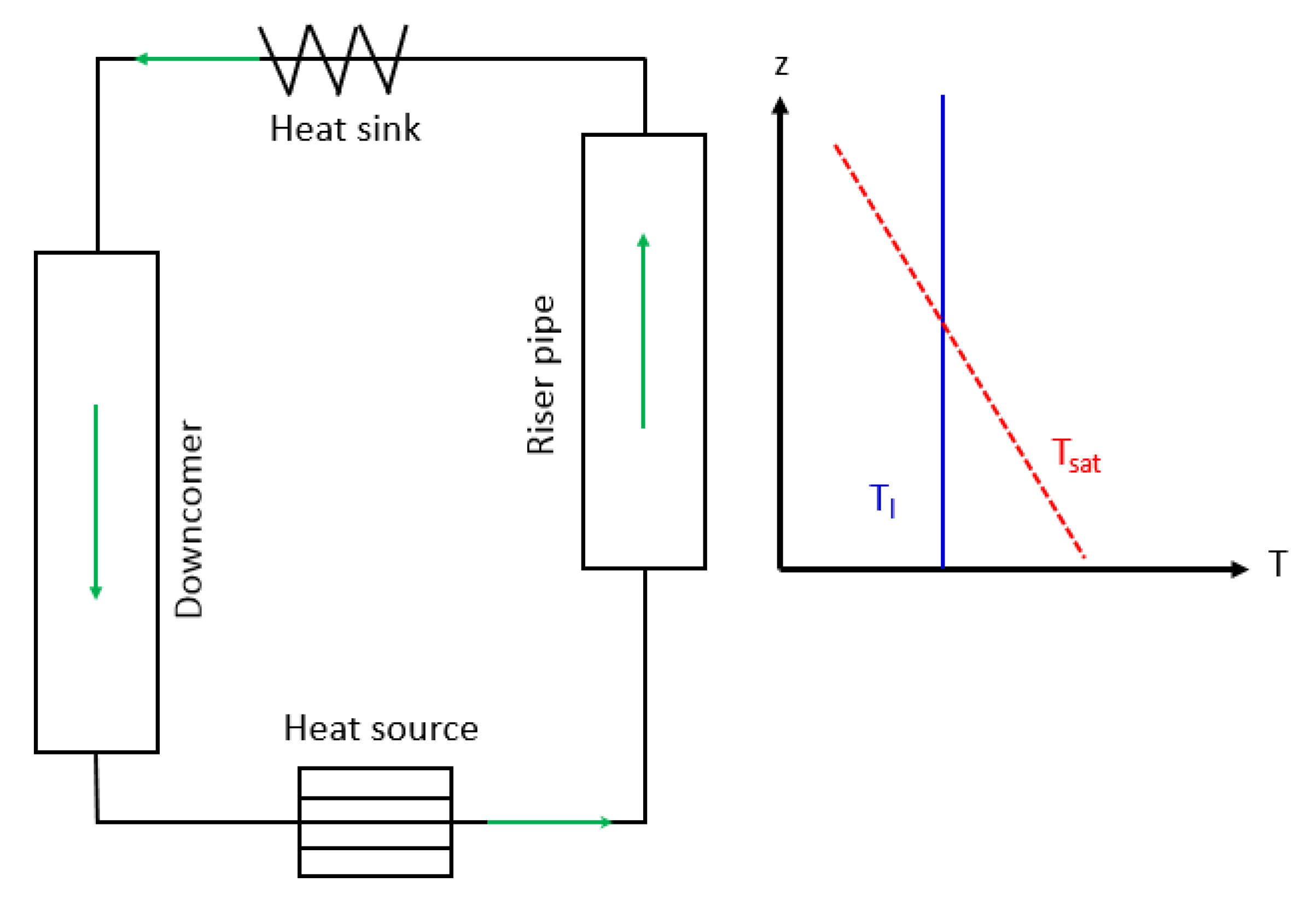
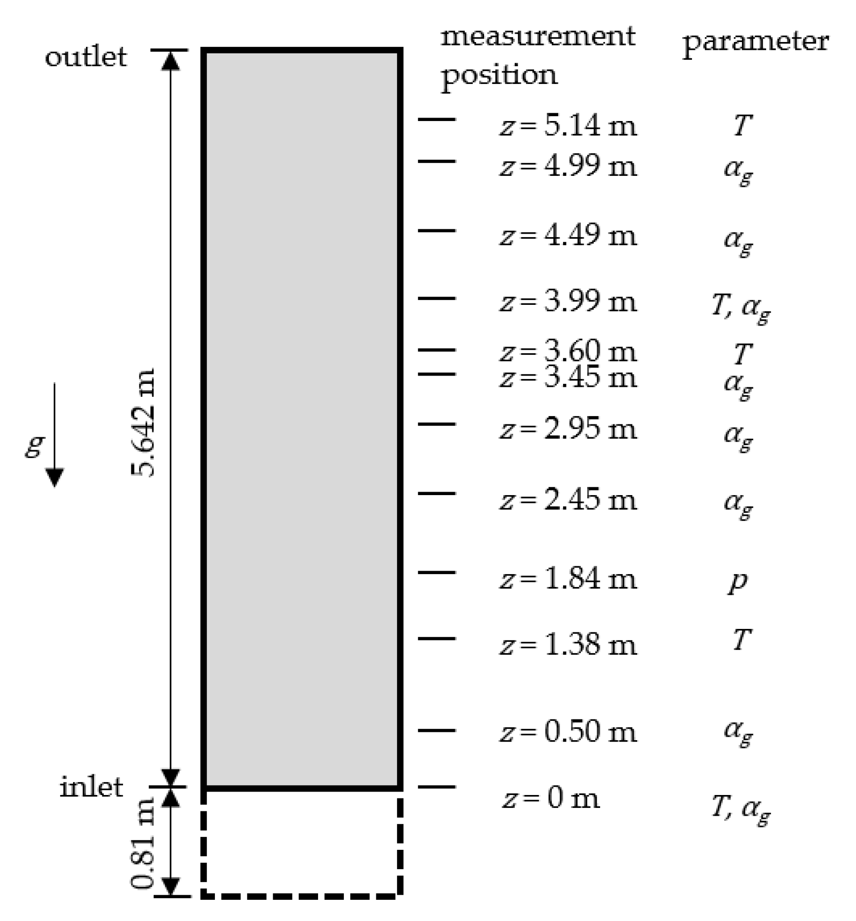
2. Test Facility and Boundary Conditions of Computational Domain

Because of its importance in nuclear safety analysis, FII has gained much attention by means of both numerical and experimental investigations [20,21,22,23,24,25,26,27]. The experiment for the present study refers to the work of Cloppenborg et al. [28], conducted at GENEVA at Dresden University of Technology, which is a semi-open natural-circulation test facility with water as the working fluid. It is built to analyze the instability behavior in the KERENA^TM reactor containment cooling condenser (CCC) system [7]. Two types of instabilities were observed, flashing and geysering, whose main difference is the point of origin. Flashing starts at the upper part of the adiabatic riser pipe due to the reduction in hydrostatic pressure, while during geysering, voids are detected at the inlet of the riser, namely boiling already occurs in the heating zone (the heat comes from the condensation of steam on the outer surface of CCC). In both situations, bubbles grow and merge intensely as they flow upward in the riser, and form large caps or slug bubbles, covering almost the whole cross-section. At the outlet of the riser, they condense rapidly in the heat sink filled with highly sub-cooled water, which results in reverse liquid flow entering the riser and high frequency fluctuations in the circuit. For the present study, a flashing case is selected for numerical studies. Considering that the test facility as well as instrumentation has been described at length in [28,29], here, only an overview of the main parameters and data used for defining the boundary conditions is given. As shown in

Table 1. Main parameters of the test circuit and the riser for the investigated case.

${\dot{\mathit{m}}}_{\mathit{m}\mathit{a}\mathit{x}}$ (kg/s)	${\mathit{T}}_{\mathit{m}\mathit{a}\mathit{x}} \left(°\mathbf{C}\right)$	${\mathit{p}}_{\mathit{m}\mathit{a}\mathit{x}}$ (bar)	${\mathit{D}}_{\mathit{r}\mathit{i}\mathit{s}\mathit{e}\mathit{r}}$ (mm)	${\mathit{L}}_{\mathit{r}\mathit{i}\mathit{s}\mathit{e}\mathit{r}}$ (m)	${\mathit{T}}_{\mathit{h}\mathit{s}}$ (°C)
~0.46	117	1.8	38	6.6	60

, in the selected case, the maximum mass flow rate during the fluctuation reaches around 0.46 kg/s, and the pressure measured at the lowest point of the circuit is about 1.8 bar. The inner diameter and length of the riser are 38 mm and 6.452 m, respectively. The water temperature in the heat sink near the outlet of the riser is 60 °C.

The part of the circuit of interest for the present study is the riser section. For the selected time segment (about 100 s), the flow at the inlet remains single-phase and constrained by the time-dependent mass flow rate and temperature profiles provided by the measurement, as shown in Figure 2. The mass flow rate fluctuates due to the occurrence of evaporation and condensation, while the temperature steadily increases about 1 K. It is worth noting that temperature fluctuation is measured at the upper part of the riser because of the reverse flow from the heat sink. Details are provided in Section 4.

For determining the pressure condition, relative pressure was measured in the middle of the riser. By considering the environment pressure as 1 atm, the absolute pressure is obtained at z = 1.84 m, which fluctuates roughly between 1.29 bar and 1.46 bar, as shown in Figure 3a. If we assume that the pressure variation along the riser is mainly dependent on the hydrostatic head and neglect the density change due to evaporation, the pressure condition at the outlet of the domain (z = 5.642 m) can be determined through $p_{out}=p_{z=1.84m}+\rho g\left(1.84 \mathrm{m}-5.642 \mathrm{m}\right)$, where g denotes the gravitational acceleration and $\rho$, the initial liquid density. The measured void fraction at the top of the riser is illustrated in Figure 3b; no bubbles were detected in the bottom region close to the inlet, which corresponds to the flash evaporation condition.

Figure 2 and Figure 3 reveal that the important features of an FII phenomenon are the high-frequency fluctuation of flow parameters, high void fractions, rapid evaporation, and condensation, which pose challenges for numerical simulations. In order to make use of the experimental data in the definition of boundary conditions, the inlet position of the computational domain is set to the lowest position, where the temperature and void fraction measurements are available, which is at a height of 0.81 m. As a result, the computational domain is 0.81 m shorter than the riser section of the test circuit, and has a length of 5.642 m (=6.452 m–0.81 m). Further details about the domain are provided in Figure 4. The data of temperature and void fraction are available at several positions, which can be used for the validation of the numerical methods. In addition, at each height position, the void fraction was measured at two radial positions, one in the center and the other, at r = 2/3R, where R is the radius of the riser pipe [28]. Compared to other experiments on FII, which have either no void fraction data or are only at one position, the GENEVA experiment is more favorable for validating the simulation results regarding the lateral void distribution.

In summary, the range of the system parameters for the simulation duration is as follows: temperature 330 ~ 378 K, pressure 0.94 ~ 2.3 bar, and void fraction 0 ~ 1.

3. Numerical Method

As discussed in the introduction, so far, most numerical analyses on FII are based on one-dimensional approaches and have clear limitations. Although there are many reports on various flashing simulations, e.g., flash atomization [30,31,32], internal nozzle flows [33,34,35,36], and leakage [37,38], CFD modeling of FII is scarce. The present study aims at exploring the transient flow behavior during the FII by means of CFD simulations. The conservation of mass, momentum, and energy is described by the means of a two-fluid model, which considers the vapor and liquid phases as two interpenetrating continua. They are coupled by interfacial terms, i.e., mass and heat transfer during the evaporation and condensation, and momentum transfer due to drag and non-drag forces. Considering that the two-fluid model for gas–liquid flows with phase change has been elaborated in many references such as [39,40], only the interfacial terms, which are the key factors affecting the results, are presented below.

3.1. Mass Transfer

After the thermodynamic equilibrium is destroyed by pressure variation, i.e., via entering the metastable zone, mass transfer associated with phase change can be driven by both pressure and temperature difference across the interface. Although there are a few attempts to consider them jointly, mass transfer in cold liquid is commonly described by a pressure phase change model, namely a cavitation model, while hot liquid is by a thermal phase change model [7]. As shown in Figure 2b, in the investigated case, the initial temperature in the riser is slightly above 100 °C. Furthermore, the reverse flow of cold water from the heat sink (60 °C) leads to intense heat exchanges between the fluids. Therefore, the thermal phase change model in ANSYS CFX is adopted in this work, which describes the phase change by interphase heat transfer and determines the interphase mass flux as:

$${\dot{m}}_{lg}=\frac{q_l+q_g}{H_{gs}-H_{ls}}$$

(1)

where ${\dot{m}}_{lg}$ denotes the mass flux flowing from gas into liquid. $q_l$ and $q_g$ represents the sensible heat flux transferring from the interface to the liquid and gas, respectively. The interfacial enthalpies $H_{gs}$, $H_{ls}$ are determined as follows:

$$H_{gs}=\{\begin{array}{c}{H}_g \mathrm{if} {\dot{m}}_{lg}>0 \\ H_{gsat} \mathrm{if} {\dot{m}}_{lg}<0 \end{array}$$

(2)

$$H_{ls}=\{\begin{array}{c}{H}_{lsat} \mathrm{if} {\dot{m}}_{lg}>0 \\ H_l \mathrm{if} {\dot{m}}_{lg}<0 \end{array}$$

(3)

where $H_{lsat}$ and $H_{gsat}$, $H_l$ and $H_g$ represent the saturation and bulk enthalpy of liquid and gas, respectively. It means that the bulk fluid enthalpy is carried out of the outgoing phase, while the saturation enthalpy is carried into the incoming phase.

3.2. Heat Transfer

The sensible heat fluxes from the interface to the fluids at both sides are computed according to:

$$q_l=h_l\left(T_i-T_l\right)$$

(4)

$$q_g=h_g\left(T_i-T_g\right)$$

(5)

In the present work, the temperature at the liquid–vapor interface is assumed equal to the saturation temperature of the vapor. Furthermore, the vapor phase is set as saturated. That means that the phase change rate is constrained only by the heat transfer between the liquid and the interface, and a reliable heat transfer coefficient is of importance. Regarding the interfacial heat transfer, it is acknowledged that the translational motion and turbulence in addition to the temperature difference play a role. Nevertheless, the interplaying of various mechanisms is far from fully understood, especially when other interactions and exchanges between the phases such as bubble-induced turbulence also become significant. There is still no generally applicable model available and numerical modeling often has to rely on empiricism to various extents. In the background of flashing flows, Liao et al. [41] conducted a thorough survey on the heat transfer mechanisms and various models. The results showed that the widely used Ranz–Marshall model is prone to under-predict the heat flux in both high superheat (Jakob number) and high turbulence conditions. Liao et al. [42] presented a mechanistic model, which consists of three parts, namely conduction, convection, and turbulence enhancement. The overall Nusselt number is expressed in a cumulative way:

$$Nu=\underset{\mathrm{conduction}}{\underbrace{\frac{12}{\pi }Ja}}+\underset{\mathrm{convection}}{\underbrace{\frac{2}{\sqrt{\pi }}P{e}^{1/2}}}+\underset{\mathrm{turbulence}}{\underbrace{\frac{2}{\sqrt{\pi }}P{e}_t{}^{1/2}\frac{d_b}{l_{turb}}}}$$

(6)

where $Nu$, $Ja$, and $Pe$ denote the Nusselt number, Jakob number, and Péclet number, respectively, and $P{e}_t$ is defined based on the turbulence velocity and length scale. It is worth noting that a similar model has been proposed by Wolfert et al. [43]:

$$Nu=\underset{\mathrm{conduction}}{\underbrace{\frac{12}{\pi }Ja}}+\underset{\mathrm{convection}}{\underbrace{\frac{2}{\sqrt{\pi }}P{e}^{1/2}}}+\underset{\mathrm{turbulence}}{\underbrace{\frac{2}{\sqrt{\pi }}P{e}^{1/2}\frac{{\lambda }_t}{{\lambda }_l}}}$$

(7)

where ${\lambda }_t$ is an adjustable parameter, referred to as eddy conductivity. Both models provide a higher heat transfer coefficient than the Ranz–Marshall one and improve the prediction at high velocity and turbulence cases according to previous studies [41]. The model of Liao et al. has been validated for bubble growth in liquid with constant superheat, condensing, and flashing steam–water pipe flows [42,44].

3.3. Interfacial Area Density

In gas–liquid flows, the interfacial transfer of momentum, heat, and mass is directly related to the contact surface between the two phases, which is characterized by the interfacial area density. ANSYS CFX provides three models for the calculation of the interfacial area density, namely the particle, mixture, and free surface model. The particle model assumes that the gas phase is present as spherical bubbles of mean diameter $d_b$, and calculates the contact area per unit volume by:

$$A_i=\frac{6{\alpha }_g}{d_b}$$

(8)

while the mixture model treats the gas and liquid phase symmetrically and expresses the interfacial area density as:

$$A_i=\frac{{\alpha }_g{\alpha }_l}{L_{mix}}$$

(9)

where the mixture length scale $L_{mix}$ must be specified by the user. The free surface model attempts to resolve the interface and obtains the interfacial area density from the gradient of the phase volume fraction, i.e.,:

$$A_i=\nabla \left|{\alpha }_l\right|$$

(10)

It is clear that an accurate calculation of the interfacial area density requires knowledge of the interfacial topological structure. In the FII process, the flow pattern inside the vertical riser pipe changes periodically from single-liquid phase, via bubbly flow to churn-turbulent or slug flow, and then reverse. Tracking the dynamic change locally and modeling the interfacial area density accordingly are both still challenging. In this work, the particle model is chosen, but instead of mean diameter, the number density of bubbles is specified, which allows the bubbles to grow and is closer to the physical picture. Equation (8) is reformulated as:

$$A_i={\left(6{\alpha }_g\right)}^{2/3}{\left(\pi N_b\right)}^{1/3}$$

(11)

by substituting the relation between $N_b$ and $d_b$. To increase the robustness further, the model is modified with regard to the following two aspects:

• The ${\alpha }_g$ is clipped to a minimum volume fraction to ensure that the area density does not reach zero;
• Because for large ${\alpha }_g$, the assumption of gas being dispersed is invalid, the area density is decreased to zero as ${\alpha }_g$ tends to 1.

$$A_i={\left[{\left(\frac{6·\max \left({\alpha }_g,{\alpha }_{g,min}\right)}{d_b}\right)}^{-2}+{\left(\frac{6{\alpha }_{g,max}}{d_b}·\frac{\max \left(1-{\alpha }_g,{\alpha }_{g,min}\right)}{1-{\alpha }_{g,max}}\right)}^{-2}\right]}^{-1/2}$$

(12)

The value for ${\alpha }_{g,min}$ and ${\alpha }_{g,max}$ is 10⁻⁷ and 0.8, respectively. It is worth mentioning that similar modifications are made in CFX by default. Figure 5 shows the change of interfacial area density with gas volume fraction obtained by the original and modified particle model. As it evidences, the model adopted in this work (given by Equation (12)) is more robust, having a minimum value at both ends, ${\alpha }_g=0$ and ${\alpha }_g=1$, and a smooth transition between the low and large ${\alpha }_g$ regimes.

The interfacial area density model has a significant influence on the results. The specification of bubble diameter or bubble number density can be regarded as limiting cases of a future more realistic model, e.g., the population balance model, which allows both quantities to vary locally [44].

Furthermore, the momentum transfer is described by the interphase drag force, which is dominant in governing the relative motion between the phases, while the non-drag forces affect only the lateral distribution of phases. The Ishii–Zuber model is adopted for the computation of drag coefficient, which takes into account the bubble shape change and swarm effects automatically. Liquid turbulence is modeled by the k-omega SST model, while a zero-equation model is applied to the gas phase by approximating the kinematic eddy viscosity with that of the liquid phase. The enhancement of shear stress and dispersion due to the presence of bubbles is accounted for by using the Sato-enhanced eddy viscosity model [45].

4. Results

The FII phenomenon inside the GENEVA riser is investigated with the boundary conditions and numerical models presented above. As aforementioned, the main feature of a FII phenomenon is a high-frequency fluctuation of flow field parameters and high-speed phase change process (evaporation and condensation). In addition, flash evaporation resulting from hydrostatic pressure reduction always starts from the uppermost part of the tube, where the pressure level is the lowest, and then propagates downward. The fluctuation and temporospatial distribution of the major parameters are presented in this section.

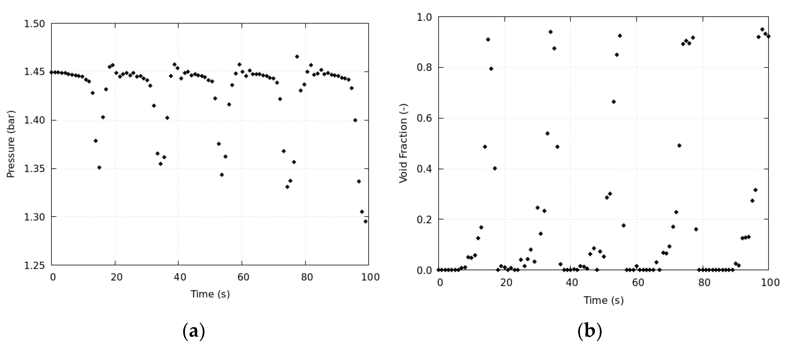
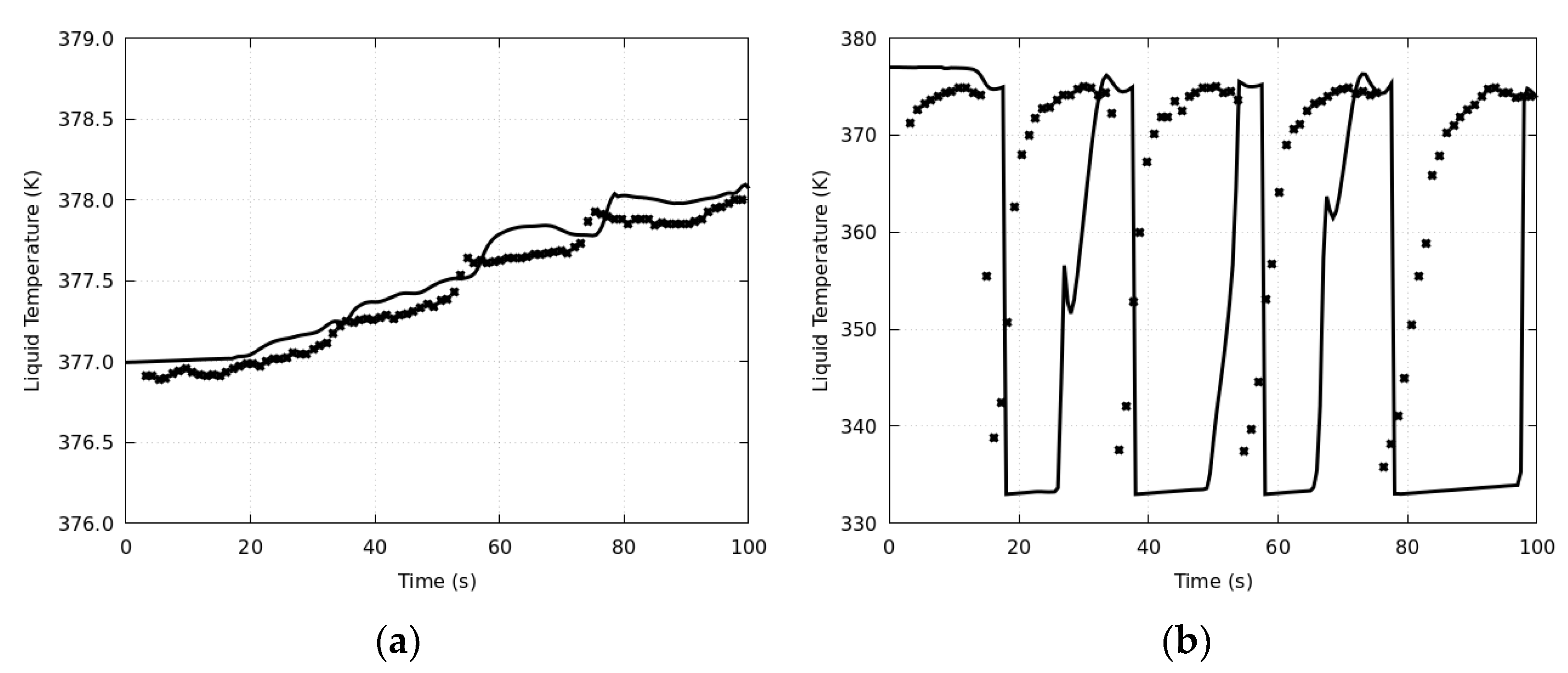
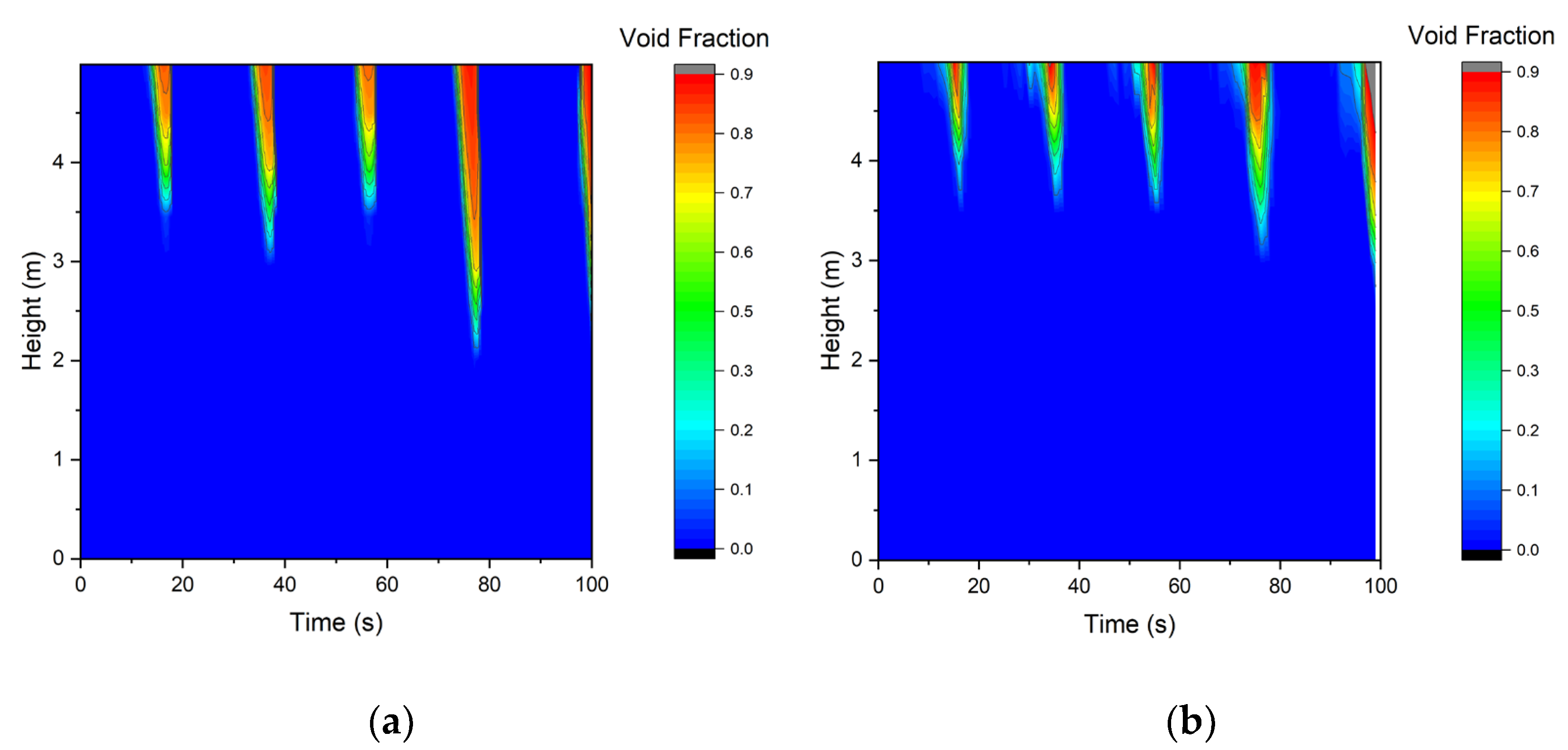
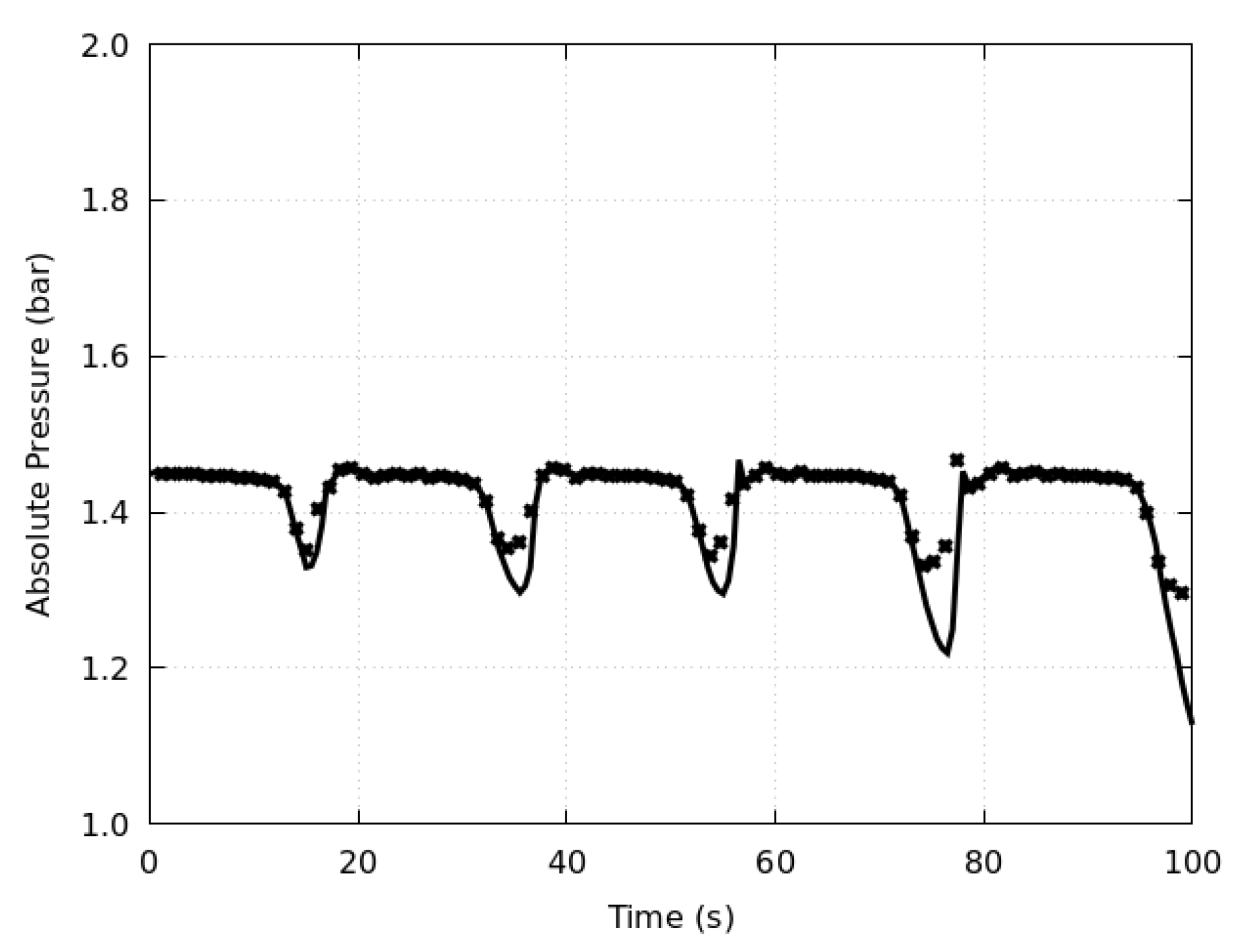
4.1. Fluctuations of Flow Parameters

The temporal change of void fraction at the height position z = 4.99 m is depicted in Figure 6, where (a) is at the pipe center (r = 0 m) and (b) at r = 2/3R with R as the pipe radius. The simulation (line) yields a flashing start later than the experiment (symbol). The moments that the peaks of void fraction appear are t = 16 s, 36 s, 56 s, 76.5 s, and 100 s in the simulation, and 14.8 s, 33.8 s, 54.8 s, 76.8 s, and 87.8 s in the experiment. It indicates that the speed of liquid temperature recovery at the condensation stage is under-predicted. In addition, the maximum void fraction reached in each period is lower according to the simulation, which is probably because the interfacial area density is clipped to zero at ${\alpha }_g=1$. The experiment measures a higher void fraction near the wall than in the center, while the simulation delivers a relatively uniform distribution over the pipe cross-section. In other words, the void fraction at r = 0 m and r = 2/3R is comparable. Nevertheless, both the experiment and simulation show a fluctuating temporal course, and the frequency conforms to each other. There appear four and a half flashing fluctuation periods (evaporation–condensation) within the 100 s simulation time.

Figure 7 presents the comparison of the pressure fluctuation at two height positions, where z = 5.642 m corresponds to the outlet of the riser. Since pressure boundary conditions have been applied to the outlet according to the experimental data, the results from simulation and experiment are in perfect match. Nevertheless, deviation is observed at z = 1.84 m. For example, the lowest value of each fluctuation cycle is smaller in the simulation than the measurement, which is associated with the under-prediction of void fraction discussed previously. A higher void fraction results in a lower average density and smaller pressure loss as the gas–liquid mixture flows along the pipe. By combining with the void fraction presented above, one can see that the decrease in pressure induces flash evaporation, while the recovery leads to condensation. While the decreasing speed of pressure is well-captured, the recovery is delayed but fast in the simulation (see Figure 7b). Another observation is that a rapid recovery of pressure tends to cause unexpected pressure peaks, e.g., around t = 20 s and 80 s, indicating numerical instability.

Due to the effect of inlet condition (see Figure 2b), the liquid temperature increases slowly before any phase change occurs in the lower part of the riser, and the variation is about 1 K (see Figure 8a). If the flashing is triggered, the evaporation leads to a temperature drop in each cycle. According to the measurement at z = 3.6 m and z = 3.99 m, the drop is up to 2 K. The numerical model adopted in this work is capable of reflecting these two kinds of temperature changes.

An important point in the semi-open natural circulation circuit is that the cold water can enter the riser from the storage pool above and cause a large temperature fluctuation in the outlet adjacent region. To simulate this phenomenon, opening boundary conditions are applied to the riser outlet. As shown in Figure 8b, both the experiment and simulation indicate the reverse flow from the storage pool at z = 5.14 m. The lowest temperature in the simulation corresponds to the prescribed 333 K, which is the temperature of the water in the storage pool, while the experiment yields a slightly higher value. A large difference is observed at the stage that the temperature recovers. The experiment shows that the temperature rises immediately after it reaches its minimum, while in the simulation, the lowest temperature lasts much longer, even up to 20 s. The discrepancy is presumably caused by two main sources of uncertainties. One is associated with the magnitude of reverse flow. Since, in the experiment, the riser is longer and the location of the storage pool is higher, the cooling effect of the reverse flow at the location of z = 5.14 m is less than that in the simulation. Another suspect is that although the heat transfer coefficient model of Liao et al. has been validated in Liao et al. [44] for both evaporation and condensation, but at low Jakob numbers, its capability for large superheat or subcooling (~40 K in this case) needs further validation.

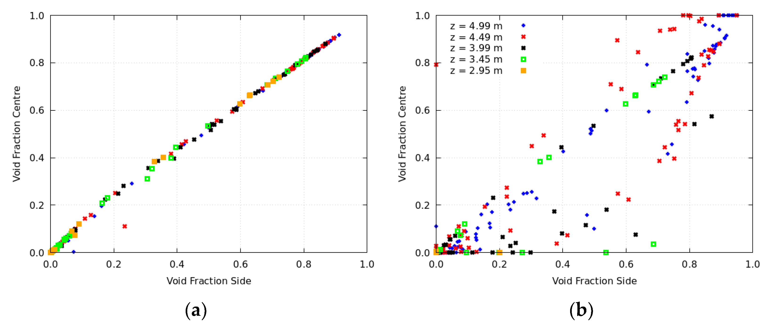
4.2. Temporospatial Distribution of Flow Parameters

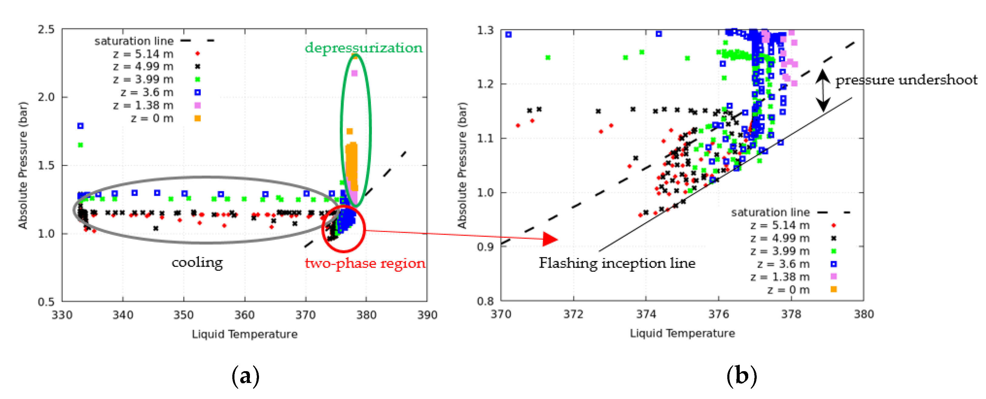
As aforementioned, the flashing evaporation is initiated at the top of the riser and then propagates downward. Figure 9 shows the change of the void fraction along the axis of the pipe with the time. The experiment indicates that the front of the void fraction waves generated in the first three flashing cycles approximately reaches a depth of z = 3.5 m. The subsequent two cycles due to the higher pressure fluctuation (see Figure 7a) lead to a longer wave. Although there are some deviations, e.g., the over-predicted wave at t = 76.5 s due to the unexpected pressure peak (see Figure 7b), the major features are successfully captured by the simulation. Both the simulation and experiment show that the void fraction peaks are narrow, indicating rapid phase change processes, especially the condensation, which is completed in 1~2 s.

After each flashing cycle, the system returns to single-phase liquid condition, and is cooled by the reverse cold flow. The intensity and duration of flash evaporation in the FII is directly affected by the local liquid temperature distribution between the cycles. Figure 10 presents the simulated and measured temperature along the axis of the riser pipe as well as its change with time. In the simulation, the cooling or reverse flow stage obviously lasts longer than that observed in the experiment, whose clarification needs further research. In contrast to the nearly uniform temperature fluctuations, an excessively strong cold flow is predicted around t = 38.5 s and t = 80 s, which reaches the depth of z = 3.66 m and z = 1.5 m, while in the experiment, the front of the cold flow ceases before z = 4.0 m (see Figure 10b). The discrepancy is associated with the pressure peaks depicted in Figure 7b. In addition, the experiment shows a slightly lower temperature close to the outlet compared to other regions at t = 0 s, which is not considered in the simulation, where instead, a uniform temperature field is assumed.

For the further analysis of the gas–liquid two-phase flow structure, the void fraction at the center and side is presented in Figure 11. The comparison between Figure 11a,b reveals a large deviation. As introduced in Section 3, the bubble number density is prescribed in the simulation (N = 5 × 10⁴ m⁻³ assumed for this study), and consequently, the Sauter mean diameter varies between 0.1 mm and 33 mm. In bubbly flows, it is known that the non-drag forces such as lift and turbulence dispersion forces affect the lateral distribution of the phases. However, considering the fact that it is difficult to describe the effect of non-drag forces accurately by means of one model for such a wide size range of bubble sizes, the non-drag forces are not included in this work. As a result, the distribution of void fraction over the cross-section is nearly uniform, and the value at the center is approximately the same on the side (see Figure 11a). On the other hand, the experiment reveals that the void fraction is higher in the area close to the pipe wall compared to the pipe center, especially at low void fraction stages and low height positions. It indicates that the wall nucleation is of importance in the early stage of flashing, and a considerable portion of small bubbles is present, which tend to accumulate in the near-wall region due to the effect of lift force.

Some characteristic parameters of the flashing cycles such as the start and end times, peak and valley values of the void fraction, pressure, and temperature are summarized in

Table 2. The start and end times, peak and valley values of the void fraction, pressure, and temperature in the first four flashing cycles.

Cycle No.		1.		2.		3.		4.
		Exp.	Sim.	Exp.	Sim.	Exp.	Sim.	Exp.	Sim.
Void fraction (at r = 0 m, z = 4.99 m)	tstart (s)	6.8	2	18.8	32.5	40.8	53.5	65.8	72
	tend (s)	17.8	18	37.8	38	56.8	58	78.8	78
	Peak value	0.91	0.827	0.94	0.848	0.926	0.818	0.917	0.885
Pressure (at r = 0 m, z = 1.84 m)	tstart (s)	3.2	1.5	26.8	29.5	44.1	48.5	66.6	70
	tend (s)	20.4	18	41.9	38.5	58	58	80.6	78.5
	Valley value (bar)	1.35	1.26	1.35	1.24	1.34	1.28	1.33	1.17
Temperature (at r = 0 m, z = 5.14 m)	tstart (s)	15	14	34.4	38	54.8	58	76.3	78
	tend (s)	20.4	33	40.8	54	63.4	69	91.4	98
	Valley value (K)	339	333	337	333	337	333	335	333

, where the measurement and simulation results are compared. The data used for the analysis are the same as shown in Figure 6a, Figure 7b and Figure 8b.

5. Discussion

In addition to instability issues caused by rapid condensation, a major challenge encountered in the numerical study of FII is that the isothermal depressurization and isobaric cooling processes are present simultaneously, as shown in Figure 12a. The former prevails at the lower part of the riser (z ≤ 3.6 m), while the latter at the upper part (z > 3.6 m). They are highlighted by the green and grey circles, respectively. Flash evaporation occurs when the pressure drops to some point below the saturation line, which is observed at the height positions larger than z = 3.6 m. The distance between the flashing inception and the saturation line is called pressure undershoot, which is about 0.1 bar in the investigated case according to the simulation. The liquid temperature decreases and pressure increases during the evaporation. Due to the joint effect of temperature decrease and pressure recovery, the liquid returns to the saturation line. After the condensation of vapor, the liquid temperature decreases isobarically and rapidly in the single-phase region, which is circled by grey in Figure 12a. On the saturation line, the liquid and vapor are in thermodynamic equilibrium, and both have the saturation pressure and temperature. If we zoom into the two-phase region (highlighted by the red circle), we can see that most datapoints are located below the saturation line (see Figure 12b), where the temperature and pressure differ from the saturation condition, and the two phases are in non-equilibrium. Both the temperature and pressure difference can drive the condition back to saturation by triggering the evaporation. Note that all the data in Figure 12 are obtained from the simulation. In the present study, the interfacial mass transfer is described by the thermal phase change model, which assumes that the phase change is induced by interphase heat transfer (see Section 2). The pressure in vapor and liquid is assumed to be equal. The inclusion of interfacial mass transfer induced by pressure difference may additionally improve the results.

Jin et al. [46] studied the heat transfer effects of cavitating and flashing flows numerically by using both pressure and thermal phase change models, which is, however, based on a homogeneous mixture model. Because of high transience in a FII phenomenon, there is normally no time for the gas and liquid mixture to reach a homogeneous flow state. The results show that the axial liquid velocity changes between −2.9 m/s and 12.6 m/s during the simulation, and the maximum relative velocity can reach 1.2 m/s. As discussed in Liao and Lucas [19], the neglect of relative motion between phases may lead to a significant under-prediction of the interphase heat and mass transfer.

Another point worth of discussion is that in the thermal phase change model, it is assumed that the interface always remains saturated, which is acceptable in most practical cases [47]. However, in a FII process, the change of pressure and temperature is usually too rapid for the interface to remain at the thermodynamic equilibrium condition. According to Kuznetsov [48], the departure of interfacial temperature from the saturation temperature can be taken into account by introducing an additional thermal resistance $R_{non}$. A simple model was proposed in [49]:

$$R_{non}=\frac{1}{h_{non}}=\frac{2-\chi }{2\chi }\frac{\sqrt{2\pi R_g}}{H_{fg}{}^2}\frac{T_{sat}{}^{3/2}}{{\rho }_g}$$

(13)

where $\chi$ is the condensation coefficient, $R_g$ is the gas constant, $H_{fg}$ is the latent heat of vaporization, and $T_{sat}$, ${\rho }_g$ are saturation temperature and gas density, respectively. $h_{non}$ is the heat transfer coefficient describing non-equilibrium phase change at the liquid–vapor interface.

In flashing flows, the flow pattern changes with the void fraction, e.g., from single-phase liquid via bubbly flow, churn-turbulent flow, and even to single-phase gas. Capturing the local transition numerically, especially when the change occurs very rapidly, still represents a challenge. In addition to extending the applicability range of closure models for interphase transfer, the modeling of bubble size and shape change is difficult. A poly-disperse simulation that account for different bubble sizes, bubble nucleation, and growth as well as bubble coalescence and breakup as described in [19] may help to improve the numerical results. Nevertheless, further information from the experiment on the evolution of bubble size is desirable. Recently, some multi-scale and multi-field approaches such as those in [50,51] have been developed, which are advantageous for the modeling of multiple regimes as well as their transition such as flashing flows.

Finally, to reduce the computational cost, the domain of CFD simulation is constrained to the riser, while analyses with system codes commonly consider the whole circuit. In the case that experimental data are not sufficient for the precise definition of all boundary conditions, the simulation results will contain uncertainties. For example, according to Figure 4, the temperature condition at the inlet (z = 0 m) is well-defined, but not at the outlet (z = 5.642 m), since the neighboring measurement positions are z = 5.14 m and the storage pool. In the simulation, the temperature of the reversal flow is assigned to the temperature at the storage pool. Since the storage pool as well as its connection with the riser is not modeled, there is a certain degree of uncertainty. If we shorten the computational domain further to 5.14 m, we can specify the temperature of incoming liquid from the outlet by the experimental data, which is several degrees higher than the storage pool. The pressure peaks in Figure 7b can be avoided and the flow field becomes more stable, as shown in Figure 13. Deviations are present only in the wave trough, where the simulated pressure is lower than the measured one. It indicates an under-prediction of the evaporation rate by the numerical model.

6. Conclusions

In the present work, the feature of FII phenomenon was studied numerically with the thermal phase change model, which is commonly used for bubbly flows. In order to validate the model properly, boundary conditions for the simulation are defined according to the experimental data. The results evidence that although there exist some quantitative deviations, the evaporation–condensation periodic phase change process is captured reasonably. The physical mechanism behind the instability is explored in depth by combining the numerical and experimental data. Furthermore, the challenges in the CFD modeling of FII, the limitations of the current numerical model as well as the possibilities of improvement in future studies are discussed. The main findings are summarized as follows:

• The applied thermal phase change and interfacial heat transfer coefficient model is able to reasonably predict the evaporation and condensation fluctuating process during FII.
• However, quantitative comparison shows that the evaporation rate is obviously under-predicted, which leads to a larger pressure drop inside the riser during the evaporation wave, and the onset of flashing is delayed.
• Instead of a uniform transverse distribution, higher void fractions are detected in the near-wall region compared to that in the pipe center. It indicates that both large and small bubbles are present, and the fraction of the latter exceeds that of the former. A poly-disperse approach taking into account bubble nucleation, growth, coalescence, and breakup is recommended for future work.
• Furthermore, during FII, the liquid and vapor are prone to have different pressures and temperatures. In addition to thermal effects, the contribution of pressure difference to the phase change rate should be taken into account.

References

1. Liao, Y.; Lucas, D. Computational modelling of flash boiling flows: A literature survey. Int. J. Heat Mass Transf. 2017, 111, 246–265. [Google Scholar] [CrossRef]
2. Cheng, W.L.; Zhang, W.W.; Chen, H.; Hu, L. Spray cooling and flash evaporation cooling: The current development and application. Renew. Sustain. Energy Rev. 2016, 55, 614–628. [Google Scholar] [CrossRef]
3. Ma, W.; Zhai, S.; Zhang, P.; Xian, Y.; Zhang, L.; Shi, R.; Sheng, J.; Liu, B.; Wu, Z. Research progresses of flash evaporation in aerospace applications. Int. J. Aerosp. Eng. 2018, 2018, 3686802. [Google Scholar] [CrossRef] [Green Version]
4. Zhang, T.; Mo, Z.; Xu, X.; Liu, X.; Chen, H.; Han, Z.; Yan, Y.; Jin, Y. Advanced Study of Spray Cooling: From Theories to Applications. Energies 2022, 15, 9219. [Google Scholar] [CrossRef]
5. Xiong, P.; He, S.; Qiu, F.; Cheng, Z.; Quan, X.; Zhang, X.; Li, W. Experimental and mathematical study on jet atomization and flash evaporation characteristics of droplets in a depressurized environment. J. Taiwan Inst. Chem. Eng. 2021, 123, 185–198. [Google Scholar] [CrossRef]
6. Toth, A.J. Modelling and optimisation of multi-stage flash distillation and reverse osmosis for desalination of saline process wastewater sources. Membranes 2020, 10, 265. [Google Scholar] [CrossRef]
7. Liao, Y.; Lucas, D. A review on numerical modelling of flashing flow with application to nuclear safety analysis. Appl. Therm. Eng. 2021, 182, 116002. [Google Scholar] [CrossRef]
8. Huggenberger, M.; Aubert, C.; Bandurski, T.; Dreier, J.; Fischer, O.; Strassberger, H.J.; Yadigaroglu, G. ESBWR related passive decay heat removal tests in PANDA. In Proceedings of the 7th International Conference on Nuclear Engineering, Tokyo, Japan, 19 April 1999. [Google Scholar]
9. Ishii, M.; Revankar, S.T.; Downar, T.; Tinkler, D.; Rohatgi, U.S. Modular and Full Size Simplified Boiling Water Reactor Design with Fully Passive Safety Systems; Purdue University: West Lafayette, IN, USA; Brookhaven National Lab. (BNL): Upton, NY, USA, 2003. [Google Scholar] [CrossRef] [Green Version]
10. Leyer, S.; Wich, M. The integral test facility Karlstein. Sci. Technol. Nucl. Install. 2012, 2012, 439374. [Google Scholar] [CrossRef]
11. Aksan, N.; Choi, J.H.; Chung, Y.J.; Cleveland, J.; D’Auria, F.S.; Fil, N.; Gimenez, M.O.; Ishii, M.; Khartabil, H.; Korotaev, K. Passive Safety Systems and Natural Circulation in Water Cooled Nuclear Power Plants; IAEA-TECDOC-1624; International Atomic Energy Agency (IAEA): Austria Vienna, 2009. [Google Scholar]
12. Hou, X.; Sun, Z.; Su, J.; Fan, G. An investigation on flashing instability induced water hammer in an open natural circulation system. Prog. Nucl. Energy. 2016, 93, 418–430. [Google Scholar] [CrossRef]
13. Manera, A. A startup procedure for natural circulation boiling water reactors. In Proceedings of the 11th International Topical Meeting on Nuclear Reactor Thermal-Hydraulics (NURETH-11), Popes’ Palace Conference Center, Avignon, France, 2 October 2005. [Google Scholar]
14. Liao, Y.; Lucas, D.; Krepper, E.; Rzehak, R. CFD Simulation of Flashing Boiling Flow in the Containment Cooling Condensers (CCC) System of KERENA™ Reactor. In Proceedings of the 21st International Conference on Nuclear Engineering, Chengdu, China, 29 July 2013; American Society of Mechanical Engineers: New York, NY, USA, 2013; Volume 55805, p. V003T10A039. [Google Scholar] [CrossRef]
15. Liao, Y.; Schuster, C.; Hu, S.; Lucas, D. CFD modelling of flashing instability in natural circulation cooling systems. In Proceedings of the 26th International Conference on Nuclear Engineering, London, UK, 22 July 2018; American Society of Mechanical Engineers: New York, NY, USA, 2018; Volume 51524, p. V008T09A026. [Google Scholar] [CrossRef]
16. Lucas, D.; Beyer, M.; Szalinski, L. Experiments on evaporating pipe flow. In Proceedings of the 14th International Topical Meeting on Nuclear Reactor Thermal-Hydraulics (NURETH-14), Toronto, ON, Canada, 25–30 September 2011. [Google Scholar]
17. IAEA. Use of Computational Fluid Dynamics Codes for Safety Analysis of Reactor Systems, including Containment. In Minutes of the Technical Meeting; IAEA: Austria Vienna, 2002; pp. 11–14. [Google Scholar]
18. Liao, Y.; Lucas, D.; Krepper, E.; Rzehak, R. Assessment of CFD predictive capacity for flash boiling. In Proceedings of the Computational Fluid Dynamics for Nuclear Reactor Safety-5 (CFD4NRS-5), Zurich, Switzerland, 9–11 September 2014. [Google Scholar]
19. Liao, Y.; Lucas, D. On numerical simulation of flashing flows. In Proceedings of the 18th International Topical Meeting on Nuclear Reactor Thermal-Hydraulics (NURETH-18), Portland, OR, USA, 18–23 August 2019. [Google Scholar]
20. Lim, S.G.; No, H.C.; Lee, S.W.; Kim, H.G.; Cheon, J.; Lee, J.M.; Ohk, S.M. Development of stability maps for flashing-induced instability in a passive containment cooling system for iPOWER. Nucl. Eng. Technol. 2020, 5, 37–50. [Google Scholar] [CrossRef]
21. Schulz, T.L. Westinghouse AP1000 advanced passive plant. Nucl. Eng. Des. 2006, 236, 1547–1557. [Google Scholar] [CrossRef] [Green Version]
22. Zhou, W.; Wolf, B.; Revankar, S. Assessment of RELAP5/MOD3. 3 condensation models for the tube bundle condensation in the PCCS of ESBWR. Nucl. Eng. Des. 2013, 264, 111–118. [Google Scholar] [CrossRef]
23. Lee, S.W.; Heo, S.; Ha, H.U.; Kim, H.G. The concept of the innovative power reactor. Nucl. Eng. Technol. 2017, 49, 1431–1441. [Google Scholar] [CrossRef]
24. Xing, J.; Song, D.; Wu, Y. HPR1000: Advanced pressurized water reactor with active and passive safety. Engineering 2016, 2, 79–87. [Google Scholar] [CrossRef] [Green Version]
25. Yang, S.K. Stability of flashing-driven natural circulation in a passive moderator cooling system for Canadian SCWR. Nucl. Eng. Des. 2014, 276, 259–276. [Google Scholar] [CrossRef]
26. Kozmenkov, Y.; Rohde, U.; Manera, A. Validation of the RELAP5 code for the modeling of flashing-induced instabilities under natural-circulation conditions using experimental data from the CIRCUS test facility. Nucl. Eng. Des. 2012, 243, 168–175. [Google Scholar] [CrossRef]
27. Wang, Q.; Gao, P.; Xu, Y.; Zhang, Y.; Lin, Y.; Wang, Z. Numerical simulation of thermal-hydraulic characteristics in a closed natural circulation system. In Proceedings of the IOP Conference Series: Earth and Environmental Science, Sanya, China, 19–21 November 2018; IOP Publishing: Bristol, UK, 2018; Volume 227, No. 2. p. 022001. [Google Scholar]
28. Cloppenborg, T.; Schuster, C.; Hurtado, A. Two-phase flow phenomena along an adiabatic riser–An experimental study at the test-facility GENEVA. Int. J. Multiph. Flow 2015, 72, 112–132. [Google Scholar] [CrossRef]
29. Manthey, R. Two-phase flow instabilities in an open natural circulation system. Ph.D. Thesis, Dresden University of Technology, Dresden, Germany, 2021. [Google Scholar]
30. Guo, H.; Torelli, R. On the effect of mixing-driven vaporization in a homogeneous relaxation modeling framework. Phys. Fluids 2022, 34, 093304. [Google Scholar] [CrossRef]
31. Sparacino, S.; Berni, F.; Riccardi, M.; Cavicchi, A.; Postrioti, L. 3D-CFD Simulation of a GDI Injector Under Standard and Flashing Conditions. In Proceedings of the E3S Web of Conferences 2020; EDP Sciences: Les Ulis, France, 2020; Volume 197, p. 06002. [Google Scholar] [CrossRef]
32. Schmidt, D.; Colarossi, M.; Bergander, M.J. Multidimensional modeling of condensing two-phase ejector flow. In Proceedings of the International Seminar on Ejector/Jet Pump Technology and Applications, Louvain-la-Neuve, Belgium, 7 September 2009. [Google Scholar]
33. Sampedro, E.O.; Breque, F.; Nemer, M. Two-phase nozzles performances CFD modeling for low-grade heat to power generation: Mass transfer models assessment and a novel transitional formulation. Therm. Sci. Eng. Prog. 2022, 27, 101139. [Google Scholar] [CrossRef]
34. Zhu, J.; Elbel, S. CFD simulation of vortex flashing R134a flow expanded through convergent-divergent nozzles. Int. J. Refrig. 2020, 112, 56–68. [Google Scholar] [CrossRef]
35. Le, Q.D.; Mereu, R.; Besagni, G.; Dossena, V.; Inzoli, F. Computational fluid dynamics modeling of flashing flow in convergent-divergent nozzle. J. Fluids Eng. 2018, 140, 101102. [Google Scholar] [CrossRef]
36. Janet, J.P.; Liao, Y.; Lucas, D. Heterogeneous nucleation in CFD simulation of flashing flows in converging–diverging nozzles. Int. J. Multiph. Flow 2015, 74, 106–117. [Google Scholar] [CrossRef]
37. Zhao, X.; Liao, Y.; Wang, M.; Zhang, K.; Su, G.H.; Tian, W.; Qiu, S.; Lucas, D. Numerical simulation of micro-crack leakage on steam generator heat transfer tube. Nucl. Eng. Des. 2021, 382, 111385. [Google Scholar] [CrossRef]
38. Jo, J.C.; Jeong, J.J.; Yun, B.J.; Kim, J. Numerical analysis of subcooled water flashing flow from a pressurized water reactor steam generator through an abruptly broken main feed water pipe. J. Press. Vessel Technol. 2019, 141, 044501. [Google Scholar] [CrossRef]
39. Liao, Y.; Lucas, D. Poly-disperse simulation of condensing steam-water flow inside a large vertical pipe. Int. J. Therm. Sci. 2016, 104, 194–207. [Google Scholar] [CrossRef]
40. Ooi, Z.J. Improved Closure Relations for the Two Fluid-Model in Flashing Flows. Ph.D. Thesis, University of Illinois at Urbana-Champaign, Champaign, IL, USA, 2020. [Google Scholar]
41. Liao, Y.; Lucas, D. Evaluation of interfacial heat transfer models for flashing flow with two-fluid CFD. Fluids 2018, 3, 38. [Google Scholar] [CrossRef] [Green Version]
42. Liao, Y.; Krepper, E.; Lucas, D. A baseline closure concept for simulating bubbly flow with phase change: A mechanistic model for interphase heat transfer coefficient. Nucl. Eng. Des. 2019, 348, 1–13. [Google Scholar] [CrossRef]
43. Wolfert, K.; Burwell, M.J.; Enix, D. Non-equilibrium mass transfer between liquid and vapour phases during depressurization process in transient two-phase flow. In Proceedings of the 2nd CSNI Specialists Meeting, Paris, France, 12–14 June 1978. [Google Scholar]
44. Liao, Y.; Lucas, D. Numerical analysis of flashing pipe flow using a population balance approach. Int. J. Heat Fluid Flow 2019, 77, 299–313. [Google Scholar] [CrossRef]
45. Sato, Y.; Sekoguchi, K. Liquid velocity distribution in two-phase bubble flow. Int. J. Multiph. Flow 1975, 2, 79–95. [Google Scholar] [CrossRef]
46. Jin, M.S.; Ha, C.T.; Park, W.G. Numerical study on heat transfer effects of cavitating and flashing flows based on homogeneous mixture model. Int. J. Heat Mass Transf. 2017, 109, 1068–1083. [Google Scholar] [CrossRef]
47. Rose, J.W. Condensation heat transfer. Heat Mass Transf. 1999, 35, 479–485. [Google Scholar] [CrossRef]
48. Kuznetsov, V.V. Non-equilibrium processes in multiphase and multicomponent microscale systems. J. Phys. Conf. Ser. 2018, 1105, 012086. [Google Scholar] [CrossRef]
49. Schrage, R.W. A Theoretical Study of Interphase Mass Transfer; Columbia University Press: New York, NY, USA, 1953. [Google Scholar] [CrossRef]
50. Mimouni, S.; Fleau, S.; Vincent, S. CFD calculations of flow pattern maps and LES of multiphase flows. Nucl. Eng. Des. 2017, 321, 118–131. [Google Scholar] [CrossRef] [Green Version]
51. Meller, R.; Schlegel, F.; Lucas, D. Basic verification of a numerical framework applied to a morphology adaptive multifield two-fluid model considering bubble motions. Int. J. Numer. Methods Fluids 2021, 93, 748–773. [Google Scholar] [CrossRef]
Figure 1. Sketch of a natural circulation circuit and saturation temperature change inside the riser pipe.
Processes 11 01974 g001
Figure 2. Time-dependent inlet (a) mass flow rate and (b) liquid temperature provided by experiment.
Processes 11 01974 g002
Figure 3. Time-dependent (a) reference pressure at z = 1.84 m and (b) void fraction at z = 4.99 m provided by experiment.
Processes 11 01974 g003
Figure 4. Geometrical details about the computational domain and measurement positions for pressure, temperature, and void fraction.
Processes 11 01974 g004
Figure 5. Change of interfacial area density with void fraction predicted by different models.
Processes 11 01974 g005
Figure 6. Fluctuation of void fraction at the center and on the side at the height position z = 4.99 m (outlet at z = 5.642 m) in the simulation duration of 100 s (symbol: experiment, line: simulation). (a) At the center (r = 0 m), (b) on the side (r = 2/3R).
Processes 11 01974 g006
Figure 7. Fluctuation of absolute pressure at two height positions in the simulation duration of 100 s (symbol: experiment, line: simulation). (a) At z = 5.642 m; (b) at z = 1.84 m.
Processes 11 01974 g007
Figure 8. Fluctuation of liquid temperature at two height positions in the simulation duration of 100 s (symbol: experiment, line: simulation). (a) At z = 1.38 m; (b) at z = 5.14 m.
Processes 11 01974 g008
Figure 9. Temporal distribution of void fraction along the axis of the pipe. (a) Simulation; (b) experiment.
Processes 11 01974 g009
Figure 10. Temporal distribution of liquid temperature along the axis of the pipe. (a) Simulation; (b) experiment.
Processes 11 01974 g010
Figure 11. Comparison of the void fraction measured at the center (r = 0 m) and the side (r = 2/3 R) of the pipe. (a) Simulation, (b) experiment.
Processes 11 01974 g011
Figure 12. Non-equilibrium effects in the FII phenomenon reflected by the relation between the liquid temperature and the absolute pressure (the dash line represents the saturation condition, the solid line in (a) represents the flashing inception line, the grey circle highlights the isobaric cooling stage due to reversal flow from heat sink, the green circle highlights the isothermal depressurization process, the red circle highlights the two-phase region, the datapoints provided by the simulation). (a) Full range, (b) zoomed two-phase region in (a).
Processes 11 01974 g012
Figure 13. Fluctuation of absolute pressure at z = 1.84 m in the simulation duration of 100 s if the domain outlet is at z = 5.14 m (symbol: experiment, line: simulation).
Processes 11 01974 g013