Study on Stimulation Mechanism and Parameter Optimization of Radial Water Jet Drilling Technique in Low Physical Property Sections of Petroleum Reservoirs

Abstract

Radial drilling-fracturing is an innovative fracturing technology that achieves superior stimulation effects. In order to study the permeability-increasing effect and main influencing factors of radial water jet drilling in the low physical section, this paper uses a fracking electrical simulation experiment, based on the principle of hydropower similarity, to simulate the reservoir conditions and well pattern in the low physical section and, at the same time, establishes the radial fracturing model of the low physical section reservoir, simulates the saturation field, pressure field, and production-change law under different drilling parameters, and studies different influencing factors. The experimental results show that when the number of drilling holes exceeds two, the effect of increasing production gradually becomes less significant as the number of drilling holes increases; Within the range of the angle between the two boreholes, the forward distance of the oil–water displacement front is the farthest and the sweep is relatively uniform. On both sides of the included angle, the forward distance of the oil–water displacement front edge is smaller than the forward distance of the displacement within the included angle range and it is clearly inclined towards the radial drilling with uneven spread. Radial drilling has an impact on the seepage field, causing changes in its streamline. The pressure inside the borehole is lower than the surrounding formation pressure and most of the flow lines change direction near the borehole location, causing deflection. As the borehole length increases, the oil-well production also increases. The optimal effect is for the borehole length to be 100 m. This study provides a reference for the on-site application of radial fracturing in low physical properties sections.

1. Introduction

With the continuous increase of oilfield water-drive development, the water cut of the oilfield is increasing, and the development of low physical property intervals is gradually receiving attention. The low physical property section refers to the formation with a thickness of less than 0.5 m and a permeability of less than 200 × 10⁻³ μm². Swartzendruber [1,2], Beavers [3], Nasser [4], Basak [5], and other scholars carried out research on non-Darcy seepage in different media such as saturated porous media, unsaturated soil, and fibrous porous media in the 1960s and 1970s. Cao [6] and others systematically introduced the characteristics of single-phase fluid, oil–water two-phase flow, and two-phase unstable flow in low physical property intervals or reservoirs, the flow law of non-Darcy flow, mathematical model, and relevant research methods. JA McCorquodale [7], Volker [8], Thauven [9], and others have described the laws of different stages of nonlinear seepage in low physical property intervals with mathematical methods and established mathematical models. Using finite element analysis, network-structure simulation, and numerical simulation to solve the critical conditions that can calculate and determine non-Darcy seepage [10,11,12]. Guppy [13], Evans [14,15], and others explored and studied the single-phase percolation characteristics and change rules of cores in low physical property intervals through experimental means, established empirical equations describing the non-Darcy percolation characteristics of low physical property intervals, and discussed the objective existence and characteristics of nonlinear percolation in low physical property intervals. Thomas [16], Fuquan [17], and others have, respectively, studied the starting pressure gradient in non-Darcy flow. They believe that when there is a starting pressure gradient, the non-Darcy low-velocity flow characteristics of a fluid in single medium and dual medium are obvious, and the pressure-curve shape of non-Darcy low-velocity flow is concave, which is greatly different from Darcy flow. Different methods, such as constant-rate mercury injection, nuclear magnetic resonance, percolation experiment, numerical experiment, and well-test interpretation can measure the non-Darcy percolation curves of low permeability cores with different permeability levels [18,19] and discuss the causes and influencing factors of the proposed starting pressure gradient. The pore-structure characteristics of the reservoir, air permeability, fluid viscosity, and movable fluid saturation have a significant impact on the starting pressure gradient of low-permeability reservoirs. The starting pressure gradient is measured by the steady or unsteady pressure-flow method and other physical simulation methods [20] and the starting pressure gradient of different seepage media is obtained, and the relationship between the starting pressure gradient and permeability, mobility, and other reservoir-fluid property parameters are clarified. For the development of a low physical property section, the cost of horizontal wells is high, the operation cycle is long, and the treatment effect of conventional fracturing and acidizing measures is not obvious. Therefore, the radial water jet drilling technology came into being and its application in the development of low physical properties can produce a significant stimulation effect. Dickinson [21,22,23] collected and analyzed the data of the initial field application of radial water jet technology and believed that the technology could achieve the effect of increasing production. Ragab [24] carried out radial water jet transformation on selected wells and believed that the effect of crude-oil stimulation was affected by reservoir physical properties and construction parameters, and the stimulation range was between 13% and 52%. Bruni et al. [25] introduced the application of radial drilling technology in two basins in the south of Argentina to study the reservoir’s physical properties and determine the construction scope. Graham [26] introduced the application case of carbonate formation in the North Urtabluk oilfield in the south of Uzbekistan using the radial water jet technology to effectively exploit the remaining oil in the formation. Chen Yuxin [27] developed a model for radial drilling-fracturing in shale reservoirs, which can predict fracture initiation pressure and the failure mode of shale. Compared with published models, this model additionally considers shale hydration and inclinations of boreholes and reservoirs; the influences of seven factors are studied.

To sum up, radial water jet technology is a drilling and completion technology that uses a high-pressure water jet to drill small holes laterally in the main hole. This technology can greatly improve the penetration depth and the contact area between the wellbore and the reservoir and can effectively improve the recovery factor. However, the research on the mechanism of increasing production and injection of this technology mostly remains at the level of numerical simulation, and the thin and poor reservoirs with low physical properties have not been verified through laboratory experiments. In this paper, the hydraulic fracturing electrical simulation experiment is used to simulate the conditions of low physical property section and well pattern, design different perforating depths and orientations, determine the saturation field, pressure field, and production-change rule and this provides a reference for the on-site application of radial fracturing in low physical properties sections.

2. Experimental Principle

2.1. Hydropower Similarity Principle

2.1.1. Ohm’s Law

The flow of current in a wire can be expressed by the following equation:

$$I=-\frac{1}{R_{\mathsf{\rho }}}\frac{\partial E}{\partial X}$$

(1)

where:

• I is current, A;
• $R_{\mathsf{\rho }}$ is specific resistance, Ω/m;
• $\frac{\partial E}{\partial X}$ is potential gradient (X is generally for area), V/m;

2.1.2. Darcy’s Law

The fluid flow in porous media follows Darcy’s law. For the stable seepage model of a single-phase incompressible liquid, it consists of the following two parts:

Equation of motion.

$$V=-\frac{K}{\mu }\mathrm{g}\mathrm{r}\mathrm{a}\mathrm{d}(p)$$

(2)

Continuity equation.

$$\mathrm{d}\mathrm{i}\mathrm{v}\left(V\right)=0$$

(3)

where:

• grad(p), div(V) is gradient and divergence;
• K is permeability, $\mathsf{\mu }\mathrm{m}$²;
• $\mu$ is liquid viscosity, mPa∙s.

Since the incompressible body is studied, it is not necessary to consider the change of liquid state, so the equation of state is not considered. When the coefficient K/μ of the two formulas in Formula (1) and (2) is equal to or proportional to R, replace Formula (1) with Formula (2), then = μ/K. That is, the specific resistance W of the model to be built is inversely related to the Y of the actual formation.

According to the law of resistance:

$$R=\rho \frac{l}{s}$$

(4)

where:

• R is resistance, Ω;
• $l$ is conductor length, m;
• S is wire full section area, m²;
• ρ is resistivity, Ω∙m;

Derived from Formula (4):

$$\rho =\frac{RS}{l}=R_{\rho }$$

(5)

Conductivity:

$$\sigma =\frac{1}{\rho }=\frac{1}{R_{\rho }S}$$

(6)

Adopt the current internationally recognized unit system MKSA (metre∙kilog-ram∙second∙ampere). The unit of σ is $S$/m (siemens/meter).

According to the Laplace equation for a steady flow, Equation (6) is expressed as:

$$\frac{\partial I}{\partial x}+\frac{\partial I}{\partial y}+\frac{\partial I}{\partial z}=0$$

(7)

For stable voltage, E:

$$\frac{{\partial }^{2}E}{\partial x}+\frac{{\partial }^{2}E}{\partial y}+\frac{{\partial }^{2}E}{\partial z}=0$$

(8)

For stable head height, H:

$$\frac{{\partial }^{2}H}{\partial x}+\frac{{\partial }^{2}H}{\partial y}+\frac{{\partial }^{2}H}{\partial z}=0$$

(9)

Analogue simulation of flow in linear bed is as follows:

Ohm’s law:

$$I=\frac{∆E}{R}=\frac{∆E}{\frac{\rho l}{S}}=\frac{S\Delta E}{\rho l}$$

(10)

where: ΔE is the potential difference, V.

Darcy’s law:

$$q=\frac{KA\Delta p}{\mu l}\times 0.0864$$

(11)

where:

• q is plane single-phase flow liquid flow, m³/d;
• A is sectional area of the plane unidirectional flow core, m²;
• Δp is pressure difference established at both ends of the core, kPa;
• $l$ is core length, m;
• μ is liquid viscosity, mPa·s;
• K is formation permeability, μm²;
• 0.0864 is the conversion factor.

Comparing Formula (10) with Formula (11), we find that I-q, ΔE-p and ρ-${\left(\frac{K}{\mu }\right)}^{-1}$ have good consistency. It can be seen that the K/μ of the simulated formation is inversely proportional to the resistivity ρ of the selected electrolyte.

2.2. Similarity Relation

In porous media, the electrical simulation model based on the principle of the steady flow of incompressible liquid must meet the relationship between various simulation elements.

2.2.1. Geometric Similarity

The ratio of the geometric parameters of the designed model to the corresponding geometric parameters of the stratum must be the same, the boundary shape must be similar, and the strict geometric similarity must meet the following conditions:

$$\frac{{(\Delta x)}_{\mathrm{m}}}{{(\Delta x)}_{\mathrm{o}}}=\frac{{(\Delta y)}_{\mathrm{m}}}{{(\Delta y)}_{\mathrm{o}}}=\frac{{(\Delta z)}_{\mathrm{m}}}{{(\Delta z)}_{\mathrm{o}}}=C_1$$

(12)

where:

• $C_1$ is geometric similarity coefficient;
• $\Delta x,\Delta y\mathrm{a}\mathrm{n}\mathrm{d}\Delta z$ are increments in the $x$, $y$, and $z$ directions, respectively;
• m and o represent model and oil layer, respectively.

2.2.2. Motion Similarity

The actual oil layer is similar to the flow-field diagram of the model; that is, the geometric shapes of the two flow-field diagrams are similar. Since the boundary of the flow area can form equipotential (pressure) lines and streamline lines, the similarity of the wall motion must also be under the condition of geometric similarity. The essence of motion similarity is that the flow velocity is consistent with the direction. In the whole flow area, the velocity ratio of the two systems should be equal. i.e.,

$$C_{\mathrm{v}}=\frac{v_{\mathrm{m}}}{v_{\mathrm{o}}}=\mathrm{c}\mathrm{o}\mathrm{n}\mathrm{s}\mathrm{t}\mathrm{a}\mathrm{n}\mathrm{t}$$

(13)

where:

• $C_{\mathrm{v}}$ is motion similarity coefficient;
• v is velocity of flow;
• m and o represent model and oil layer, respectively.

2.2.3. Pressure Similarity

The ratio of the potential difference between two electrodes in the simulation model and the pressure difference between two corresponding points in the simulation oil layer is equal to a fixed value. i.e.,

$$C_{\mathrm{p}}=\frac{{(\Delta V)}_{\mathrm{m}}}{{(\Delta p)}_{\mathrm{o}}}$$

(14)

where:

• $C_{\mathrm{p}}$ is pressure similarity coefficient;
• ${(\Delta p)}_{\mathrm{o}}$ is pressure difference between two points in the reservoir, Pa;
• ${(\Delta V)}_{\mathrm{m}}$ is potential difference between two points of corresponding oil layer in the model, V.

2.2.4. Flow Similarity

The simulation model is similar to the reservoir flow, that is

$$C_{\mathrm{q}}=\frac{I_{\mathrm{m}}}{Q_{\mathrm{o}}}$$

(15)

where:

• $C_{\mathrm{q}}$ is flow similarity coefficient;
• $I_{\mathrm{m}}$ is current in the model, A;
• $Q_{\mathrm{o}}$ is flow in the reservoir, m³/s.

2.2.5. Resistance Similarity

In fact, when the geometric similarity, pressure similarity, and flow similarity are satisfied between the model and the reservoir, the flow resistance of current and the resistance of seepage in the reservoir must also be similar.

$$C_{\mathrm{r}}=\frac{R_{\mathrm{m}}}{R_{\mathrm{f}\mathrm{o}}}$$

(16)

where:

• $C_{\mathrm{r}}$ is resistance similarity coefficient;
• $R_{\mathrm{m}}$ is current flow resistance in the model;
• $R_{\mathrm{f}\mathrm{o}}$ is fluid-flow resistance in the oil reservoir.

According to Ohm’s law:

$$\frac{{(\Delta V)}_{\mathrm{m}}}{I_{\mathrm{m}}{R}_{\mathrm{m}}}=1$$

(17)

According to Darcy’s law:

$$\frac{{(\Delta p)}_{\mathrm{m}}}{Q_{\mathrm{o}}{R}_{\mathrm{f}\mathrm{o}}}=1$$

(18)

From Formula (14), ${(\Delta V)}_{\mathrm{m}}$ = $C_{\mathrm{p}}{(\Delta p)}_{\mathrm{o}}$, $I_{\mathrm{m}}$ = $C_{\mathrm{q}}{Q}_{\mathrm{o}}$ in Formula (15), and according to Formula (16), R_m = C_rR_fo, substitute the above into Formula (17), and use Formula (18) to get.

$$\frac{{(\Delta V)}_{\mathrm{m}}}{I_{\mathrm{m}}{R}_{\mathrm{m}}}=\frac{C_{\mathrm{p}}{(\Delta p)}_{\mathrm{o}}}{C_{\mathrm{q}}{Q}_{\mathrm{o}}{C}_r{R}_{\mathrm{f}\mathrm{o}}}$$

(19)

That is.

$$C_{\mathrm{p}}=C_{\mathrm{q}}{C}_r$$

(20)

This proves that the pressure similarity coefficient is equal to the product of the flow similarity coefficient and the resistance similarity coefficient.

3. Experimental Device and Equipment

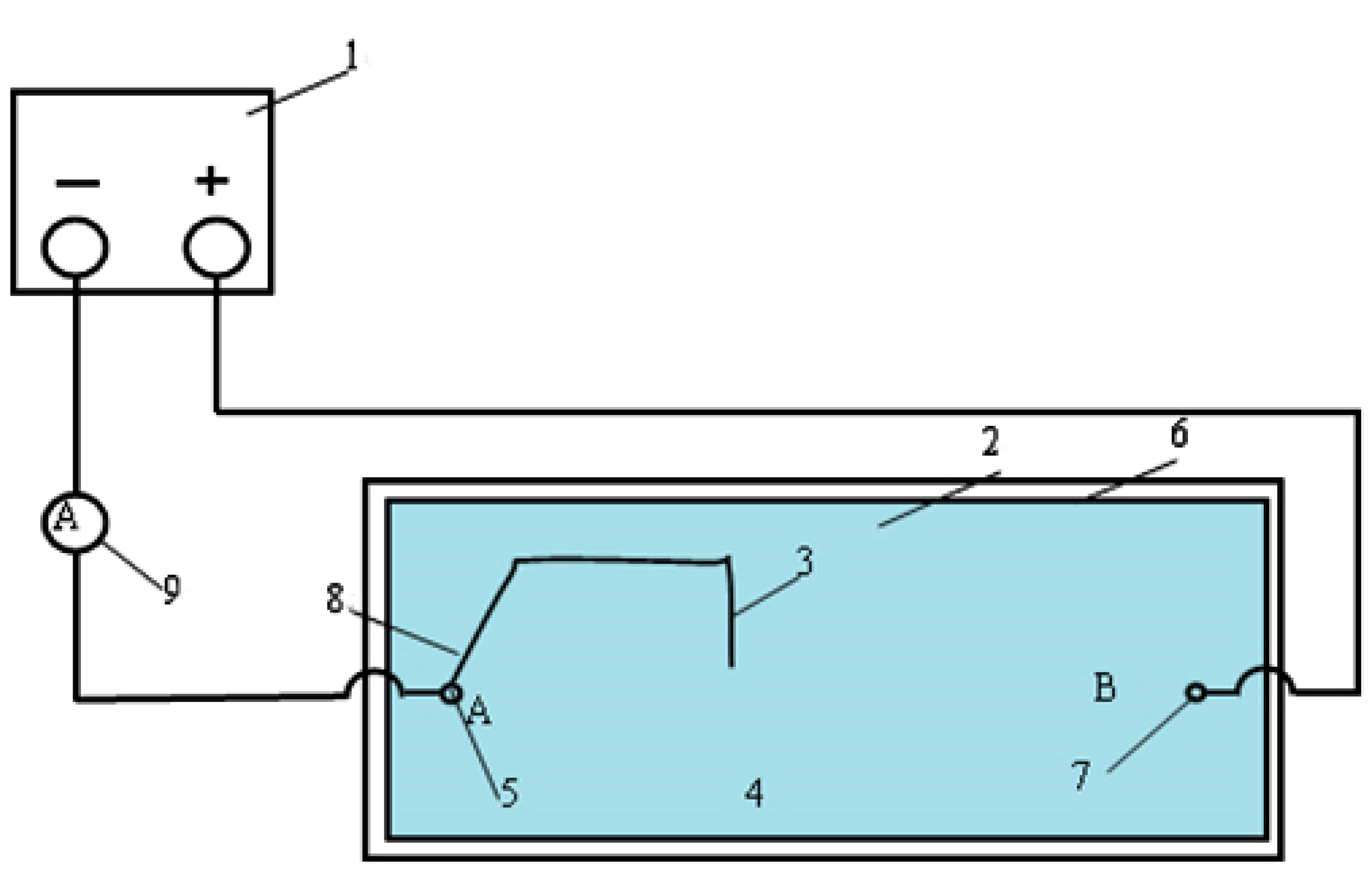
3.1. Electrical Analog Device

The electrical simulation device in the experiment is shown in Figure 1.

A three-dimensional mechanical measuring device is designed for this device. Through the horizontal bar, when hand wheel 10 is turned, the measuring probe can move longitudinally within the existing depth range and the parameters of each point can be measured. If you want to change the lateral distance, you can turn handwheel 9. Therefore, the parameters of each point in the model plane can be measured under the existing depth conditions. If you want to change the depth, you can measure the scale and handwheel 5 vertically, and use the probe to measure the parameters at each point in the rectangle of the experimental model.

The corresponding formation permeability is simulated by the configured copper sulfate concentration, and the radial water jet drilling is simulated by the iron wire put into the copper sulfate solution pool. The measured voltage value represents the formation pressure, and the current value represents the production. The impact of the radial water jet drilling on the production of a low physical reservoir is analyzed by measuring the change in the current value.

3.2. Measuring Device Circuit

Figure 2 is the circuit diagram of this experimental model. The power supply can provide stable voltage. The permeability of different formations is simulated by different concentrations of copper sulfate solution. In addition, the monitoring equipment can accurately display the parameters, such as the voltage supplied by the model, the depth of the probe entering the copper sulfate solution, the transverse distance of the probe, the longitudinal distance of the probe, and the voltage value of the detection point.

4. Factors Affecting the Stimulation of Radial Water Jet Drilling in Low Physical Property Section

The hydraulic fracturing electrical simulation experiment is used to simulate the conditions of low physical property section and well pattern, design different perforating depths and orientations, and determine the saturation field, pressure field, and production-change rule.

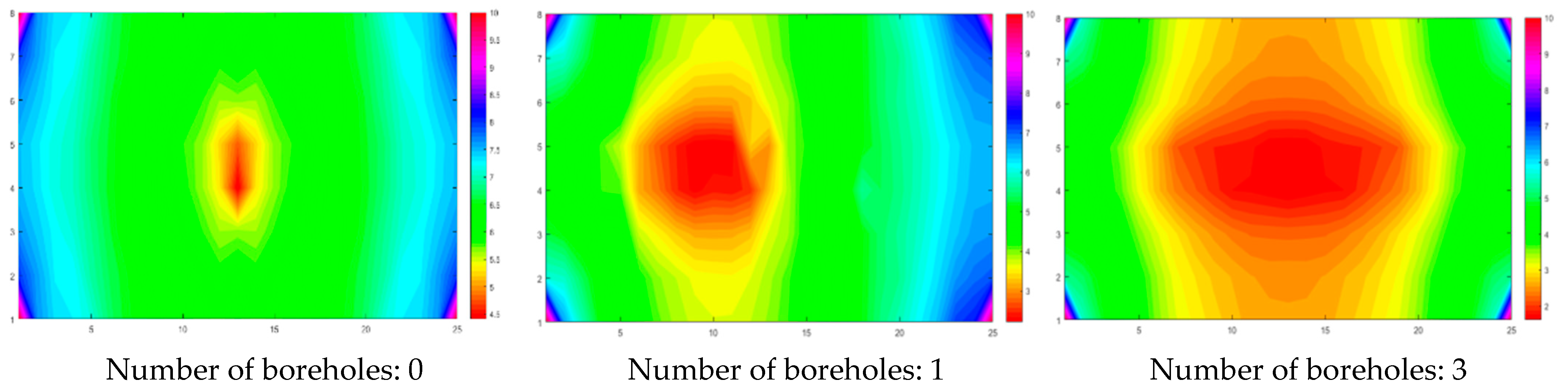
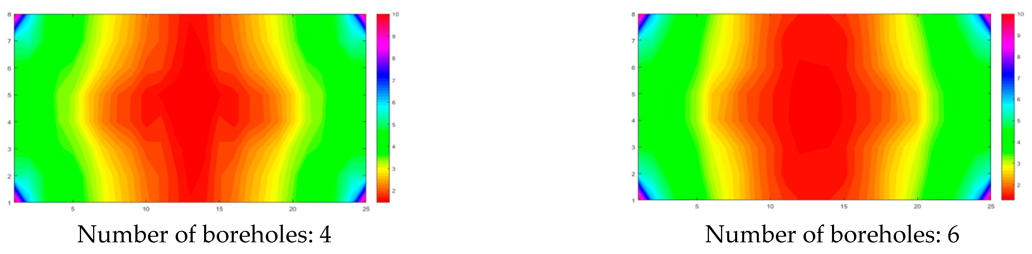
4.1. Number of Boreholes

(1)

Pressure distribution

It can be seen from Figure 3 that radial water jet drilling can change the formation-pressure distribution, reduce the interwell pressure loss and improve the displacement pressure gradient. Thus, the streamline mode of formation seepage can be changed, and the radial flow can be changed into linear flow.

(2)

Current value

With the increase in the number of boreholes, the output of each radial borehole and vertical wellbore decreases but the total productivity increases with the increase of the number and the increase is smaller and smaller. The analysis shows that the number of boreholes increases and the interference between boreholes is serious, resulting in the reduction of productivity of each borehole. However, due to the increase in the number of boreholes, the total production capacity increased. Too many boreholes will aggravate the formation pollution and the cost is too high, so the number of boreholes should be reasonably selected.

With the increase in the number of boreholes, that is, the increase of the hole density, the degree of recovery will increase. This is due to the increase of the oil drainage area and the decrease of the pressure near the bottom of the well, which leads to the increase of the liquidity, which leads to the large amount of oil being driven out. However, there is no simple linear relationship between them. This is because, with the increase of the hole density, the interference between various branches will also increase.

For some strip-shaped and thin-layer residual oil, conventional measures are difficult for tapping the potential. It is necessary to learn from unconventional mining ideas, use complex technologies such as hydraulic jet radial drilling, and combine with moderate-scale fracturing to explore personalized and vectorized “normal-normal combination” efficient potential tapping technology to achieve accurate potential tapping of highly scattered residual oil.

It can be seen from Figure 4 that after the number of boreholes is more than two, the effect of increasing production gradually becomes less obvious with the increase in the number of boreholes. Therefore, the recommended optimal number of boreholes is two.

4.2. Drilling Angle

According to the hydropower similarity theory and Ohm’s law and Darcy’s law, the corresponding relationship between copper sulfate resistivity and permeability can be obtained and copper sulfate resistivity is related to its concentration; that is, there is a functional relationship between copper sulfate concentration and permeability.

The 0.5 g/L copper sulfate solution is selected to simulate the formation with a permeability of 50 mD and the iron wire with a diameter of 2.5 mm and length of 35 cm is selected to simulate the drilling hole with a length of 100 m.

(1)

Pressure distribution

It can be seen from Figure 5 that no matter whether the included angle between the two boreholes is 60°, 90°, 120°, or 180° [27], within the range of the included angle between the two boreholes, the advance distance of the front edge of oil and water displacement is the farthest and the spread is relatively uniform. However, within the two sides of the included angle, the advance distance of the oil–water displacement front is smaller than that of the displacement within the included angle, it is obviously inclined to the radial drilling, and the sweep is not very uniform. The displacement effect is the worst in the range opposite to the drilling direction. Therefore, when the included angle of the borehole is 180°, the drive effect in each quarter block is the same and the sweep is relatively uniform.

(2)

Current value

As shown in Figure 6,With the increase of the included angle of the two boreholes, the total productivity increases and the output of each radial borehole increases but the increase is less and less. The analysis shows that the smaller the drilling angle is, the smaller the influence range of the radial borehole on the reservoir is, and the interference of the pressure field and the seepage field of the two radial boreholes will also increase with the decrease of the included angle, resulting in poor development effect. Therefore, the included angle of the two boreholes will be 180° during the radial drilling so that the mutual interference between the boreholes is small, thus improving the recovery degree. Therefore, the drilling effect is best when the drilling angle is 180°.

4.3. Borehole Length

The 0.5 g/L copper sulfate solution is selected to simulate the formation with the permeability of 50 mD and the iron wire with a diameter of 2.5 mm and length of 35 cm, 28 cm, 21 cm, 40 cm, and 7 cm is selected to simulate the borehole with length of 100 m, 80 m, 60 m, 40 m, and 20 m.

(1)

Pressure distribution

It can be seen from Figure 7 that along the radial drilling direction, the extent of water drive is relatively high and the formation pressure is significantly lower than that in other directions. In addition, the pressure range of radial drilling wells is wider than that of vertical wells and it is easier to establish an effective displacement pressure difference between wells. The longer the length, the lower the formation pressure. This is because the longer the drilling length is, the larger the oil supply area can be drilled, and the effective range of oil production wells can be increased. The radial drilling has an impact on the seepage field and changes its streamline. The pressure in the borehole is lower than the surrounding formation pressure and most of the flow lines change direction near the borehole location and deflect. When the borehole length is relatively small, the seepage mode is similar to radial flow in the whole area and the flow line converges at the end; when the drilling length is increased, the fluid turns to the drilling position because this will reduce the energy consumption. This results in parallel unidirectional flow around the radial water jet borehole and, at this time, the flow lines at the end are less concentrated. With the increase of drilling length, the influence range of parallel one-way flow will expand.

(2)

Current value

It can be seen from Figure 8 that the current value increases with the increase of the drilling length, and the best effect is when the drilling length is 100 m. The analysis shows that the longer the length is, the larger the equivalent radius (the equivalent effect on pressure caused by a well diameter) is, the wider the influence of the horizontal section of the radial drilling is, the more dominant the radial drilling is, and the obvious stimulation effect is.

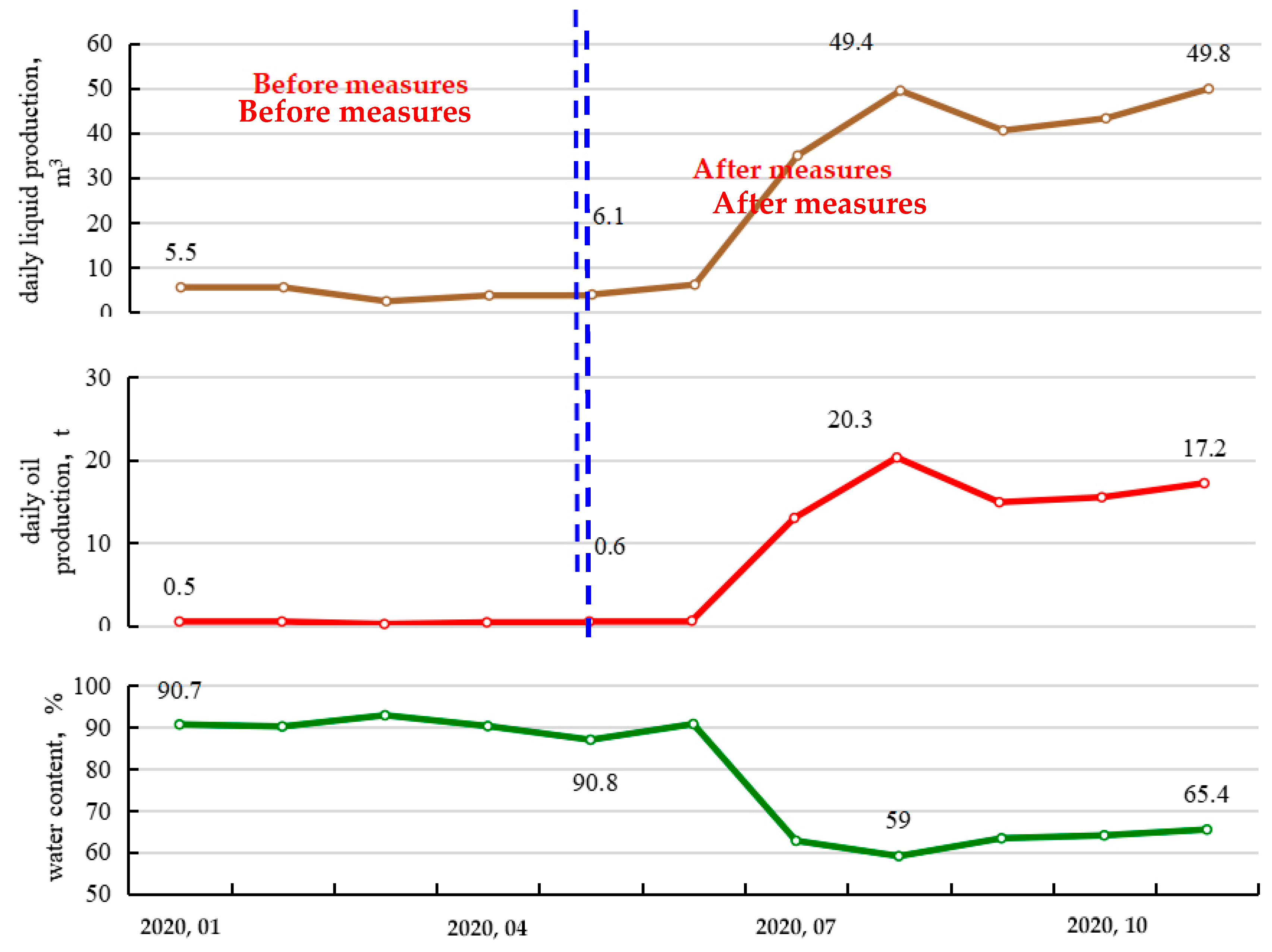
5. Field Application

In combination with the North 2-Ding6-426 well in the North 2 pilot area, directional drilling will be carried out in June 2020 with an initial daily oil increase of 1.6 t. In July 2020, fracturing will be carried out on the su-layer of SaSan5 in the directional drilling, with an oil increase of 4.1 t and an oil increase of 1002 t.

As shown in Figure 9,Through the comparison before and after the implementation of radial water jet technology, it can be seen that after the measures, the water content has decreased, the oil production has significantly increased, and the daily oil production has increased by 40 times. This indicates that radial water jet technology can effectively reduce the water content of the reservoir and improve the recovery rate of low physical properties.

6. Conclusions

(1)

The length, angle, and number of boreholes are the main factors that affect the yield order and increase the effect. The longer the drilling length, the larger the equivalent radius and the more obvious the stimulation effect. Moreover, radial drilling has an impact on the seepage field, causing changes in its flow line. The pressure inside the drilling hole is lower than the surrounding formation pressure and most flow lines change direction and deviate near the drilling position. The larger the drilling angle, the wider the impact of radial drilling on the reservoir and the better the development effect. However, the interference between the pressure and seepage fields of the two radial drilling holes will also increase with the decrease of the included angle, leading to a worse development effect. The total production capacity will increase as the number of boreholes increases but the increase will be smaller and smaller;

(2)

Under constant pressure differential production conditions, when other parameters are the same, with the increase of formation thickness, the production of each radial borehole and the production of vertical wellbore increase. Therefore, when using radial water jet drilling to develop low permeability reservoirs, the formation needs to have a certain thickness so that the development effect can be significantly improved;

(3)

Through the analysis of perforation parameters, it can be concluded that the optimal number of boreholes is two, and the optimal borehole length is 100 m when the optimal borehole angle is 180°.

References

1. Swartzendruber, D. Non-Darcy flow behavior in liquid-saturated porous media. J. Geophys. Res. 1962, 67, 5205–5213. [Google Scholar] [CrossRef]
2. Swartzendruber, D. Non-Darcy Behavior and the Flow of Water in Unsaturated Soils1, 3. Soil Sci. Soc. Am. J. 1963, 27, 491–495. [Google Scholar] [CrossRef]
3. Beavers, G.; Sparrow, E. Non-Darcy flow through fibrous porous media. J. Appl. Mech. 1969, 36, 711–714. [Google Scholar] [CrossRef]
4. Nasser, M.S. Radial non-Darcy Flow through Porous Media. Master’s Thesis, University of Windsor, Windsor, ON, Canada, 1970. [Google Scholar]
5. Basak, P. Non-Darcy flow and its implications to seepage problems. J. Irrig. Drain. Div. 1977, 103, 459–473. [Google Scholar] [CrossRef]
6. Cao, G.; Cheng, Q.; Wang, H.; Bu, R.; Zhang, N.; Wang, Q. Percolation Characteristics and Injection Limit of Surfactant Huff-n-Puff in a Reservoir. ACS Omega 2022, 7, 30389–30398. [Google Scholar] [CrossRef] [PubMed]
7. McCorquodale, J.A. Finite Element Analysis of Non-Darcy Flow; University of Windsor: Windsor, ON, Canada, 1970. [Google Scholar]
8. Volker, R.E. Solutions for unconfined non-Darcy seepage. J. Irrig. Drain. Div. 1975, 101, 53–65. [Google Scholar] [CrossRef]
9. Thauvin, F.; Mohanty, K. Network modeling of non-Darcy flow through porous media. Transp. Porous Media 1998, 31, 19–37. [Google Scholar] [CrossRef]
10. Zeng, Z.; Grigg, R. A criterion for non-Darcy flow in porous media. Transp. Porous Media 2006, 63, 57–69. [Google Scholar] [CrossRef]
11. Huang, H.; Ayoub, J.A. Applicability of the Forchheimer equation for non-Darcy flow in porous media. Soc. Pet. Eng. J. 2008, 13, 112–122. [Google Scholar] [CrossRef]
12. Rubin, B. Accurate simulation of non Darcy flow in stimulated fractured shale reservoirs. In Proceedings of the SPE Western Regional Meeting, Anaheim, CA, USA, 27–29 May 2010; Society of Petroleum Engineers: Richardson, TX, USA, 2010. [Google Scholar]
13. Guppy, K.; Cinco-Ley, H.; Ramey, H.J., Jr. Effect of non-Darcy flow on the constant-pressure production of fractured wells. Soc. Pet. Eng. J. 1981, 21, 390–400. [Google Scholar] [CrossRef]
14. Evans, R.; Hudson, C.; Greenlee, J. The effect of an immobile liquid saturation on the non-Darcy flow coefficient in porous media. SPE Prod. Eng. 1987, 2, 331–338. [Google Scholar] [CrossRef]
15. Wang, X.; Thauvin, F.; Mohanty, K. Non-Darcy flow through anisotropic porous media. Chem. Eng. Sci. 1999, 54, 1859–1869. [Google Scholar] [CrossRef]
16. Thomas, L.; Katz, D.; Tek, M.R. Threshold pressure phenomena in porous media. Soc. Pet. Eng. J. 1968, 8, 174–184. [Google Scholar] [CrossRef]
17. Fuquan, S.; Ciqun, L.; Fanhua, L. Transient pressure of percolation through one dimension porous media with threshold pressure gradient. Appl. Math. Mech. 1999, 20, 27–35. [Google Scholar] [CrossRef]
18. Prada, A.; Civan, F. Modification of Darcy’s law for the threshold pressure gradient. J. Pet. Sci. Eng. 1999, 22, 237–240. [Google Scholar] [CrossRef]
19. Fuquan, S.; Renjie, J.; Shuli, B. Measurement of threshold pressure gradient of microchannels by static method. Chin. Phys. Lett. 2007, 24, 1995. [Google Scholar] [CrossRef]
20. Hao, F.; Cheng, L.S.; Hassan, O.; Hou, J.; Liu, C.Z.; Feng, J.D. Threshold pressure gradient in ultra-low permeability reservoirs. Pet. Sci. Technol. 2008, 26, 1024–1035. [Google Scholar] [CrossRef]
21. Dickinson, W.; Dickinson, R.W. Horizontal Radial Drilling System. In Proceedings of the SPE Western Regional Meeting, Bakersfield, CA, USA, 23–25 March 1985. [Google Scholar]
22. Dickinson, B.W.O.; Dickinson, R.W.; May, S.C.; Mackey, C.S. Hydraulic Drilling Apparatus and Method. U.S. Patent US4852668, 1 August 1989. [Google Scholar]
23. Dickinson, W.; Dykstra, H.; Nees, J.M.; Dickinson, E. The Ultrashort Radius Radial System Applied to Thermal Recovery of Heavy Oil. In Proceedings of the SPE Western Regional Meeting, Bakersfield, CA, USA, 30 March–1 April 1992. [Google Scholar]
24. Ragab, A.M.S. Radial Drilling Technique for Improving Well Productivity in Petrobel-Egypt. In Proceedings of the North Africa Technical Conference & Exhibition, Cairo, Egypt, 15–17 April 2013. [Google Scholar]
25. Bruni, M.; Biasotti, J.; Salomone, G. Radial Drilling in Argentina. In Proceedings of the Latin American & Caribbean Petroleum Engineering Conference, Buenos Aires, Argentina, 15–18 April 2007. [Google Scholar]
26. Wall, G. Technologies to Develop Mature Oil Fields. In Proceedings of the Uzbekistan International Oil & Gas Exhibition and Conference, Tashkent, Uzbekistan, 14–16 May 2011. [Google Scholar]
27. Chen, Y.; Ding, Y.; Liang, C.; Zhu, D.; Bai, Y.; Zou, C. Initiation mechanisms of radial drilling—Fracturing considering shale hydration and reservoir dip. Energy Sci. Eng. 2021, 9, 113981. [Google Scholar] [CrossRef]
Figure 1. Electrical simulation device for fracturing corresponding to injection-production well. 1—Stabilized power supply; 2—Data collector (connected to a computer acquisition system); 3—Controller; 4—Electric motor; 5—Vertical handwheel; 6—Probe; 7—Production well; 8—Vertical cracks; 9—Horizontal handwheel; 10—Rectangular solution container.
Processes 11 02029 g001
Figure 2. Circuit diagram of fracturing electrical simulation experimental device corresponding to injection-production well. 1—Regulated power supply; 2—Supply boundary; 3—Probe; 4—Copper sulfate solution; 5—Produced well (A Well point); 6—electric tank; 7—Injection well (B Well point); 8—Wireway; 9—Ammeter.
Processes 11 02029 g002
Figure 3. Variation of pressure distribution with the number of boreholes.
Processes 11 02029 g003aProcesses 11 02029 g003b
Figure 4. Current value of different drill holes.
Processes 11 02029 g004
Figure 5. Variation of pressure distribution with borehole angle.
Processes 11 02029 g005
Figure 6. Current values at different angles.
Processes 11 02029 g006
Figure 7. Variation of pressure distribution with borehole length.
Processes 11 02029 g007
Figure 8. Change of current value in different drilling lengths.
Processes 11 02029 g008
Figure 9. Production Curve of Well Bei 2-Ding 6-426.
Processes 11 02029 g009
Disclaimer/Publisher’s Note: The statements, opinions and data contained in all publications are solely those of the individual author(s) and contributor(s) and not of MDPI and/or the editor(s). MDPI and/or the editor(s) disclaim responsibility for any injury to people or property resulting from any ideas, methods, instructions or products referred to in the content.