Prediction Model of Fouling Thickness of Heat Exchanger Based on TA-LSTM Structure

Abstract

Heat exchangers in operation often experience scaling, which can lead to a decrease in heat exchange efficiency and even safety accidents when fouling accumulates to a certain thickness. To address this issue, manual intervention is currently employed to monitor fouling thickness in advance. In this study, we propose a two-layer LSTM neural network model with an attention mechanism to effectively learn fouling thickness data under different working conditions. The model accurately predicts the scaling thickness of the heat exchanger during operation, enabling timely human intervention and ensuring that the scaling remains within a safe range. The experimental results demonstrate that our proposed neural network model (TA-LSTM) outperforms both the traditional BP neural network model and the LSTM neural network model in terms of accuracy and stability. Our findings provide valuable technical support for future research on heat exchanger descaling and fouling growth detection.

1. Introduction

A heat exchanger is a device used to transfer heat from one medium to another for purposes such as temperature regulation or heat recovery [1,2,3,4]. Heat exchangers are widely used in various industries, including refrigeration, heating, air conditioning, oil cooling, water cooling, and more [5,6]. The classification of heat exchangers is generally based on factors such as working conditions, fluid media, operating temperature, and pressure [4,7]. They can be categorized based on their purpose, such as heat exchangers, coolers, condensers, evaporators, and heaters. They can also be classified based on the principle of heat transfer, including direct contact heat exchangers, heat storage heat exchangers, inter-wall heat exchangers, and intermediate heat carrier-type heat exchangers.

In the heat transfer process, heat is transferred between two media through a heat transfer surface, which helps maintain a heat balance. One medium gains heat while the other loses heat. This process is accompanied by a gradual scaling phenomenon, where fluid deposits on or erodes the surface of the heat exchanger, forming a layer of solid or soft mud-like precipitate [8]. The type of fouling formed during operation varies depending on the heat exchanger’s operating conditions [9]. The current internationally accepted classification of fouling, proposed by Epstein [10], categorizes fouling into seven types based on the causes of fouling formation. These types include precipitation fouling, corrosion fouling, biofouling, particulate fouling, chemically reacted fouling, solidified fouling, and mixed fouling.

The formation of fouling is a complex process [11]. Epstein categorized the process into five stages: initiation, transportation, attachment, exfoliation, and aging. In his study, he observed a changing pattern in the thermal resistance of fouling over time. He identified three types of fouling characteristic curves: linear, descending, and asymptotic. Later, Garrett [12] and his colleagues discovered that there was a period of time without fouling formation after the initial onset. Epstein later referred to this period as the fouling induction period.

The fouling mechanism includes thermodynamic change theory, adsorption theory, and crystallization kinetics theory, which explains the causes of fouling generation at the theoretical level. At the same time, there are many factors affecting heat exchanger fouling. The structure of the heat exchanger, the heat exchanger medium, and the flow characteristics of the fluid in the heat exchanger all accelerate or inhibit the generation of fouling to different degrees.

The thermal conductivity of fouling is significantly lower than that of the parent material of the heat exchanger, making it a poor conductor of heat [13]. Research shows that more than 90% of heat exchangers experience fouling problems to varying degrees [14,15]. The presence of fouling has a detrimental impact on the normal operation of heat exchanger equipment, such as reducing heat transfer efficiency, increasing energy consumption, shortening equipment lifespan, and compromising equipment safety [16]. Currently, there are several methods available for heat exchanger descaling, including physical, chemical, and ultrasonic methods [17]. The choice of descaling method depends on the specific heat exchanger and working environment.

Ma Guangxing et al. [18] conducted an experimental study on the descaling of heat exchanger fouling at different growth stages. The study found that intervening during the induction and growth phases of fouling not only inhibits the growth rate of fouling but also reduces energy consumption and improves the descaling effect.

The descaling effect varies during different periods of fouling formation. Duan Peiqing introduced an online anti-fouling and descaling method [19,20]. However, the research on determining when the heat exchanger should be descaled and maintained is still in its early stages. In this paper, we propose an improved LSTM neural network to predict the thickness of scaling in heat exchangers. This allows us to detect the growth of scaling and determine the optimal timing for human intervention. This, in combination with the use of online descaling methods, allows the heat exchanger to operate with a certain level of fouling reduction. This extends the equipment’s service life and reduces energy consumption.

The TA-LSTM model [21,22] differs from the traditional BP model and ordinary LSTM model, as it incorporates a two-layer LSTM structure along with the attention mechanism. Unlike the BP and traditional LSTM models, the TA-LSTM model addresses the issue of disappearing or exploding gradients when dealing with long sequences, which hinders the ability to capture long-distance dependencies [23]. By introducing the attention mechanism, the TA-LSTM model effectively understands the long-distance dependencies in sequences and enhances its modeling capability for data with long sequences. The attention mechanism enables the model to assign different weights to different parts of the input, based on contextual information, thereby improving the model’s accuracy. The two-layer LSTM structure [24,25] allows the first layer to capture low-level features, which are then processed as inputs in the second layer. This enables the model to capture rich data features, making it more suitable for processing complex sequence data. Consequently, this model outperforms both the BP model and the LSTM model. Its superiority becomes more evident as the volume of data increases.

2. Theoretical Foundations

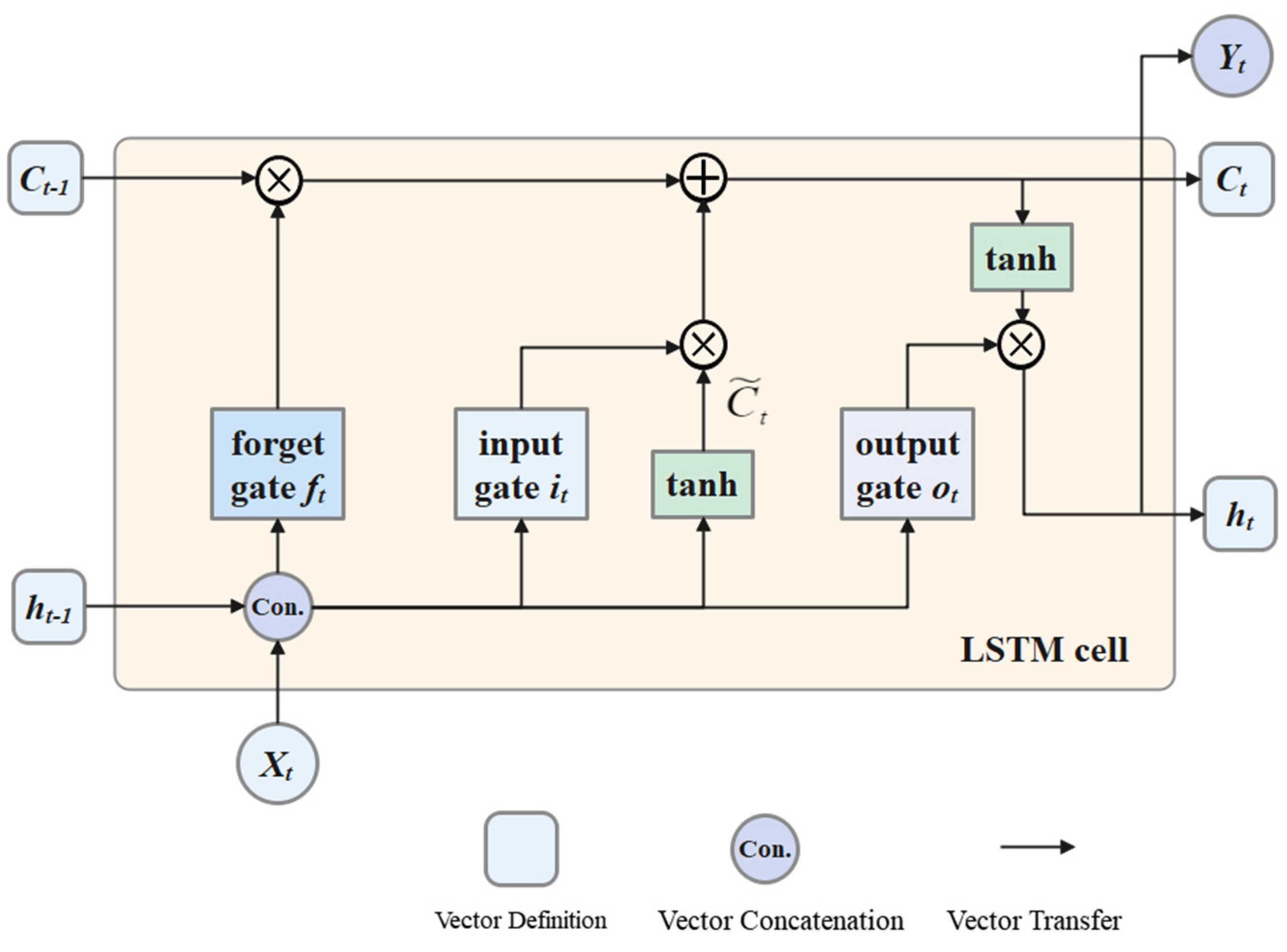
2.1. Long and Short-Term Memory Networks

An LSTM (long short-term memory) neural network is a special kind of recurrent neural network, which was proposed by Hochreiter and Schmidhuber [26] and has been improved and popularized by many people. It adds a gating mechanism [27,28] to the recurrent neural network, including forgetting gates, input gates, and output gates, which control the flow of information, enabling the network to effectively deal with long-term dependencies, and it can effectively solve the problem of gradient vanishing and gradient explosion during training of long sequences, to better realize the modeling and prediction of time series.

The structural framework diagram of the LSTM network is shown in Figure 1.

The LSTM model mainly consists of oblivion gates, input gates, cell states, and output gates. Taking the example at time step t, the input at this time can be expressed as $x_t$, then, the implied state at the previous time step is $h_{t-1}$, and the unit cell state is $c_{t-1}$.

First, the forgetting gate determines what useless information needs to be discarded from the previous cell state, i.e., the degree of forgetting. With the sigmoid cell of the forgetting gate, the comparison of $x_t$ and $h_{t-1}$ of the information, a vector between 0 and 1, is output. The values in this vector determine $c_{t-1}$ whether the information in it is retained or not. The larger the value, the higher the level of retention, with 1 indicating complete retention. The mathematical expression for this is:

$$f_t=\sigma \left(W_f\left[h_{t-1,},x_t\right]+b_f\right)$$

(1)

In this context, σ refers to the sigmoid activation function. $W_f$ represents the weight matrix of the forgetting gate, while $b_f$ represents the bias vector of the forgetting gate.

The input gate, denoted as $i_t$, determines what new information to add to the cell state and controls the extent of the input of new information. This is expressed mathematically as:

$$i_t=\sigma \left(W_i\left[h_{t-1},x_t\right]+b_i\right)$$

(2)

In this context, σ is the sigmoid activation function, $W_i$ is the input $x_t$ weight matrix of the input gate, and $b_i$ is the bias vector of the input gate.

The next step is to utilize $h_{t-1}$ and $x_t$; a new candidate cell state is obtained through a tanh layer, ${\tilde{C}}_t$. Its mathematical expression is:

$${\tilde{C}}_t=tanh\left(W_c\left[h_{t-1},x_t\right]+b_c\right)$$

(3)

In this context, $W_c$ is the input $x_t$ the weight matrix of the inputs, $b_c$ is the bias matrix, and tanh is the hyperbolic tangent activation function.

Finally, the current cell state is computed, $C_t,$ and updates the hidden state, $h_t$. Its mathematical expression is:

$$C_t=\left(f_t\ast C_{t-1}+i_t\ast C_t\right)$$

(4)

$$h_t=\left(O_t\ast tanh\left(C_t\right)\right)$$

(5)

$$O_t=\sigma \left(W_o\left[h_{t-1},x_t\right]+b_o\right)$$

(6)

In this context, * denotes the element-by-element product, and $O_t$ denotes the output gate, which is used to control the degree of output. $W_o$ is the input, $x_t,$ of the output gate matrix, and $b_o$ is the bias vector of the output gate.

2.2. Attention Mechanisms

The attention mechanism is a technique based on artificial neural networks that aids models in learning to selectively focus on specific parts when processing large amounts of information [29]. It draws inspiration from the attention mechanism of the human brain, where individuals consciously concentrate on important elements while disregarding insignificant details. This allows the human brain to gather as much valuable information as possible while conserving energy and making efficient use of resources.

Similarly, the attention mechanism can assist the model in comprehending and structuring the input information, thereby enhancing the model’s performance. In the context of neural networks, the attention mechanism assigns weights to each input feature based on its similarity to the current state. This allows for the activation of inputs with varying degrees of similarity, which are then combined to create a new feature representation.

When predicting the thickness of heat exchanger fouling, the collected individual input data may deviate from the actual value due to experimental errors. To ensure the accuracy of the neural network model, it is important to eliminate the influence of irrelevant input data on the prediction results. To achieve this, an attention mechanism is introduced in the LSTM model. This mechanism enables the model to effectively handle long sequences, address ambiguities, and tackle more complex tasks.

The paper discusses two types of attention mechanisms: the hard attention mechanism (HAM) and the soft attention mechanism (SAM) [30]. In this study, the soft attention mechanism [31] is employed to allocate the weight value of attention within the range of [0, 1]. The calculation of this weight value is demonstrated in the following equation:

In this paper, the soft attention mechanism is used to distribute the weight value of attention between [0, 1], which is calculated as shown in the following equation:

$$softmax\left(z_i\right)=\frac{e^{Z_i}}{\sum _{i=1}^n{e}^{Z_i}}$$

(7)

In this context, $Z_i$ denotes the value of the ith position in the input sequence, and n denotes the number of categories contained in the sequence.

The steps of the attention mechanism are as follows:

(1)

Encoder: converts the input sequence into an intermediate representation, e.g., processed using the LSTM model.

(2)

Calculate attention weights: given the current decoder state and intermediate representations, calculates the weights or distributions for each input element, indicating the degree of importance.

(3)

Weighted summation: weighted summation of intermediate representations based on attention weights to obtain weighted information.

(4)

Decoder: generates the current output based on the weighting information as well as the previous memory, while updating the decoder status and previous memory.

(5)

Repeat steps two through four until the complete output sequence is generated.

2.3. Two-Layer LSTM Neural Network

Bilayer LSTM [32] is a type of deep recurrent neural network that comprises two LSTM layers. In this architecture, the first LSTM layer takes the input sequence and produces a hidden state, which can be seen as an intermediate representation capturing information from the input sequence. This hidden state is then passed to the second LSTM layer, which utilizes it to further process the information.

Training a two-layer LSTM model typically requires more computational resources compared to a single layer. However, increasing the number of layers enhances the expressive power of the model, enables capturing longer time dependencies, and improves its overall performance.

3. Introduction to the Model

This study proposes the use of a joint attention mechanism and a two-layer LSTM (TA-LSTM) [33] to enhance the performance of neural networks in sequence modeling and processing tasks. By employing a two-layer LSTM network, the model can capture long-term dependencies and contextual information in sequences. Additionally, the attention mechanism enables the network to dynamically prioritize important parts of the sequences. The structure of the proposed model is illustrated in Figure 2.

The workflow is as follows:

(1)

The input sequence is processed through the first LSTM layer to produce the hidden state, $h_t$, and cell state sequences, $c_t$.

(2)

A soft attention mechanism is introduced in the first LSTM layer to compute attention weights and attention up and down vectors.

(3)

The attention up and down vectors, $c_t$, are combined with the hidden state of the first LSTM layer, $h_t$, to be merged to get the new hidden state, $h_t^{\prime }$.

(4)

The new hidden state, $h_t^{\prime },$ is used to perform further processing and input the second LSTM layer.

(5)

Further operations are performed in the second LSTM layer to obtain the final hidden state sequence, $h_t^{\prime \prime },$ and the cell state sequence, $C_t^{\prime \prime }$.

(6)

Predictions are obtained by the final sequence of hidden states, $y_t$.

4. Experimentation

4.1. Subjects and Samples

The fields of ship heat exchangers and aircraft heat exchangers are characterized by demanding cost control [34], energy saving and emission reduction [35], stability, and safety. Taking aircraft heat exchangers as an example, they play a vital role in regulating the temperature and humidity inside the aircraft. Due to the unique working environment and safety requirements of aircraft heat exchangers, it is crucial to ensure that the fouling thickness remains within a safe range during airplane operation. When the scale thickness exceeds 1mm, it can result in reduced heat transfer efficiency, higher outlet temperature, and pollution [36,37]. Therefore, the TA-LSTM model is well-suited for predicting the fouling thickness of aircraft heat exchangers, enabling timely human intervention to eliminate safety hazards.

In this paper, the experimental data of Linying Du [38] on the heat exchangers on Boeing 737-800 model airplanes were selected to carry out model training and prediction. Four experimental factors that have the greatest influence on fouling were selected as the model input. They are ambient temperature, air conditioning system inlet pressure, primary heat exchanger outlet pressure, and secondary heat exchanger outlet pressure.

Figure 3 shows a diagram of the air conditioning and refrigeration system of the Boeing 737-800, where the ambient temperature is the final airliner air conditioning outlet temperature. The inlet pressure is the pressure of the high-temperature and high-pressure pilot gas produced by the engine when it passes through the FCSOV. The primary outlet temperature is the temperature of the airflow through the primary heat exchanger, and the secondary outlet temperature is the temperature of the airflow through the secondary heat exchanger. Some samples from the experiment are shown in

Table 1. Partial experimental data. (This data is cited in the following literature [38]).

Brochure	Serial Number	Environmental Temperature (°C)	Inlet Pressure (Pa)	Initial Temperature (°C)	Secondary Effluent Temperature (°C)	Scale Thickness (mm)
Network training samples	1	35	100	59	38.1	0.48
	2	25	100	76	53.3	0.93
	3	25	100	97	81.0	1.12
	4	25	30	59	38.1	0.38
	5	35	100	76	53.3	0.92
	6	25	30	97	81.0	1.08
	7	25	60	59	38.1	0.47
	8	25	60	76	53.3	0.9
	9	35	100	97	81.0	1.07
	10	30	30	59	38.1	0.45
	11	30	30	97	81.0	1.02
	12	30	100	59	38.1	0.5
	13	30	100	76	53.3	0.93
	14	30	100	97	81.0	1.1
	15	30	60	59	38.1	0.45
	16	30	60	76	53.3	0.88
	17	35	60	59	38.1	0.41
Sample Network Test	18	35	30	59	38.1	0.46
	19	35	30	76	53.3	0.83
	20	35	30	97	81.0	0.99
	21	25	100	59	38.1	0.52
	22	25	30	76	53.3	0.85
	23	30	30	76	53.3	0.91
	24	35	60	97	81.0	1.11
	25	35	100	97	81.0	1.07

(This data is cited in [38]).

4.2. Experimental Platform and Experimental Environment

The environment and platform required for the experiment are shown in

Table 2. Experimental platform and experimental environment.

Experimental Environment	Specific Information
Operating system	Windows 10
Processing unit	Intel(R) Xeon(R) Platinum 8373C CPU @ 2.60 GHz 2.60 GHz (2 processors)
Display card (computer)	NVIDA GeForce RTX 3050
Random access memory (RAM)	256G
Programming language	Python
Development environment (computer)	Pytorch
Development tool	Pycharm

.

4.3. Experimental Model Evaluation Metrics

This paper utilizes the TA-LSTM prediction model, which consists of an attention mechanism combined with a two-layer LSTM network. The evaluation metrics [39] employed in this study are MAPE, MAE, and RMSE. In this context, n represents the number of samples, $y_i$ denotes the true value of the ith sample, and $\widehat{y_i}$ represents the predicted value of the ith sample.

1.

Mean Absolute Percentage Error (MAPE)

$$\frac{100\%}{n}\sum _{i=1}^n\left|\frac{y_i-{\widehat{y}}_i}{y_i}\right|$$

(8)

MAPE (mean absolute percentage error) is a metric that quantifies the average percentage difference between the predicted fouling thickness and the true fouling thickness. It is commonly employed to assess the accuracy of prediction models, particularly for narrower ranges of true values.

In this context, n represents the number of samples, $y_i$ denotes the true value of the ith sample, and $\widehat{y_i}$ represents the predicted value of the ith sample.

2.

Mean Absolute Error (MAE)

$$\frac{1}{n}\sum _{i=1}^n\left|y_i-{\widehat{y}}_i\right|$$

(9)

The MAE (mean absolute error) represents the average difference between the true fouling thickness and the predicted fouling thickness. It is a measure used to quantify the average prediction error of the model. A smaller MAE indicates that the predicted value is closer to the true value.

In this context, n represents the number of samples, $y_i$ denotes the true value of the ith sample, and $\widehat{y_i}$ represents the predicted value of the ith sample.

3.

Root Mean Square Error (RMSE)

$$\frac{1}{\sqrt{n}}\sqrt{\sum _{i=1}^n{\left(y_i-{\widehat{y}}_i\right)}^2}$$

(10)

The RMSE (root mean square error) represents the average difference between the true fouling thickness and the predicted fouling thickness. It is a metric that is more sensitive to outliers compared to other metrics.

In this context, n represents the number of samples, $y_i$ denotes the true value of the ith sample, and $\widehat{y_i}$ represents the predicted value of the ith sample.

4.4. Experimental Steps

Step 1. The different magnitudes of the original data and the inevitable existence of abnormal values and vacant data will affect the authenticity of the prediction results. Therefore, for the selected experimental data, the realm temperature, T, inlet pressure, P, primary outlet temperature, $T_1$, and secondary outlet temperature, $T_2$, are normalized to meet the input requirements.

Step 2. The experimental data is divided into two parts in chronological order; the former is used to train the model, and the latter is used to adjust the hyper-parameters, thus determining the input and output variables of the model.

Step 3. A random search with the PSO algorithm is used to find the optimal parameters.

Step 4. After completing the stochastic initialization of the weight matrix of the TA-LSTM prediction model, the data can be input.

Step 5. In training the model, optimization is performed by the Adam optimizer and evaluated using the loss function, RMSE.

4.5. Analysis of Forecast Results

Figure 4 presents the training error and testing error of the TA-LSTM model. The model proposed in this paper predicts the fouling thickness of aircraft heat exchangers after deep learning in the test set. The error curves, depicted in the figure, show that the training error curve (red curve) consistently surpasses the testing error curve (blue curve), indicating a significant improvement in the model’s prediction accuracy after deep learning from the test set. Moreover, as the number of iterations increases, both the training error curve and the test error curve demonstrate a substantial reduction, eventually converging to a thickness close to the true value. This convergence point satisfies the requirements of engineering practice.

MAPE, MAE, and RMSE are commonly used metrics to evaluate the performance of neural network models [40,41]. To reflect the superiority of the model in one step, this paper adopts the MAPE, MAE, and RMSE evaluation indexes to evaluate the prediction performance of the traditional BP model, the LSTM model, and the TA-LSTM model, respectively, within the traditional BP model, the LSTM model, and the TA-LSTM model. The metrics are shown in

Table 3. Indicators for evaluation of models.

Group	MAPE	RMSE	MAE
BP	0.07127	0.07298	0.06157
LSTM	0.02374	0.02049	0.01481
TA-LSTM	0.00231	0.00168	0.00136

and Figure 5.

Comparing the analysis metrics of the three models, the traditional BP model performs the worst, followed by the ordinary LSTM model, and the TA-LSTM model performs the best. The table and figure clearly show that the evaluation index values of the TA-LSTM model are significantly smaller than those of the BP model and lower than those of the ordinary LSTM model. Among these metrics, a smaller MAPE value indicates a better model type. The RMSE value is penalized more for samples with larger prediction errors, so a smaller value indicates lower variance and better model performance. The MAE value measures the absolute value of the average prediction error without considering its direction and is relatively less penalized for larger error samples. All three metrics consistently demonstrate the superiority of the TA-LSTM model.

Figure 6 presents the performance of the three models in predicting the data from the validation set in Table 1. The horizontal and vertical coordinates represent different input data in the validation group, with the vertical coordinate indicating the thickness of the dirt in millimeters. The true error of the model is determined by the difference between the y-coordinate of the predicted and true values of the three models at the same horizontal coordinate.

It is not difficult to find that the curve trends of the three models can roughly match the direction of the true value curve. Among them, the traditional BP curve will appear to be extremely unstable, stage by stage away from the true curve. And the predicted value is lower than the true value. Among them, in the ordinary LSTM model, the performance is still good, basically in line with the trend of the real value, the accuracy, and the TA-LSTM, but there is a certain gap. The model adopted in this paper has the best performance, which is not only the closest to the real value, but also has no abnormal prediction float, so it is the most reliable.

5. Conclusions

This paper proposes a two-layer LSTM neural network model, based on the attention mechanism, for analyzing and concluding the following points:

• The paper selects four main factors, namely ambient temperature, air conditioning system inlet pressure, primary heat exchanger outlet pressure, and secondary heat exchanger outlet pressure, which affect the growth of heat exchanger fouling. This multi-feature input method effectively represents the fouling growth environment.
• By introducing the attention mechanism to calculate the time series and adaptively allocate weights based on the input information, the model improves its robustness and generalization ability. This process aligns with the growth process of heat exchanger fouling over time, thereby significantly enhancing the prediction accuracy of the model.
• This model utilizes a two-layer LSTM structure along with an attention mechanism. This design not only enhances the model’s expressive capability but also enables it to capture longer time dependencies, resulting in improved performance.
• When comparing the errors between the predicted values of the three models and the experimental true values, it is observed that the BP model performs the worst, followed by the LSTM model, and the present model performs the best. The predicted value curve of the present model demonstrates the closest fit to the real value curve and exhibits the most stable behavior without abnormal fluctuations. Furthermore, the evaluation indexes (MAPE, MAE, and RMSE) of the TA-LSTM model show an improvement of over 40% compared to those of the common LSTM model. This improvement validates the reliability and stability of the TA-LSTM model, which fulfills the requirements of engineering practice. Consequently, the TA-LSTM model can play a significant role in the field of heat exchanger fouling growth detection and heat exchanger descaling.

6. Prospects and Challenges

The current mainstream descaling methods for heat exchangers often require post-treatment downtime, resulting in long downtimes and affecting production continuity and efficiency. This is particularly inconvenient in areas such as ships and airplanes. Therefore, the future direction of development should focus on integrated heat exchanger cleaning methods that incorporate online scale inhibition and descaling.

By combining the researchers’ subsequent study of the fouling growth cycle, this technology can predict the optimal time for human intervention by determining the thickness of the fouling. This provides technical support for online scale inhibition and descaling methods and can even help simulate fouling growth, providing fouling growth curves for future work.

Implementing the model requires a significant amount of fouling data as a basis. The more data collected, the more accurate the prediction results will be. Therefore, the pre-collection of data will be a crucial task in future research, but it also poses a challenge.

References

1. Liu, J. A review of research on the current status and future trend of heat exchanger development. China Equip. Eng. 2022, 510, 261–263. [Google Scholar]
2. Hu, H.; Zhang, L.; Huang, W.; Li, G. Classification and development trend of automotive heat exchanger. Automot. Eng. 2015, 3, 15–17. [Google Scholar] [CrossRef]
3. Zhang, X. Development status and future development trend of heat exchanger industry. Mass Invest. Guide 2019, 1–5. [Google Scholar]
4. Gao, G.; Zhang, X.; Li, C. Current status of research and development of heat exchanger. Contemp. Chem. Res. 2016, 83–84. [Google Scholar]
5. Liu, J. Exploration of future development trend of heat exchanger industry. China Mark. 2016, 3, 61+64. [Google Scholar] [CrossRef]
6. Hu, B.; Xia, Z. Development status and outlook of China’s heat exchanger industry. Comput. Prod. Circ. 2017, 12, 1. [Google Scholar]
7. Lv, M.; Yang, X.; Zhang, Y.; Zhuang, Y. Analysis of the current situation of heat exchanger and classification application. Contemp. Chem. Ind. 2018, 47, 582–584. [Google Scholar]
8. Yin, X.; Chen, Y.; Song, Y. Progress in the study of fouling characteristics in heat exchangers. Chem. Equip. Technol. 2021, 42, 1–6. [Google Scholar]
9. Shang, Y.; Cai, X.; Liu, X.; Zhang, J.; Xiao, D.; Ouyang, Z.; Zhang, Y.; Zhang, W. Research on the implementation program of on-line cleaning of heat exchangers. Petrochem. Equip. 2012, 41, 4–7. [Google Scholar]
10. Epstein, N. Fouling in Heat Exchangers. In Proceedings of the International Heat Transfer Conference 6, Toronto, ON, Canada, 7–11 August 1978. [Google Scholar] [CrossRef]
11. Li, Y. Research on Fouling Growth Characteristics of Direct Sewage Source Heat Pump; Xi’an University of Architecture and Technology: Xi’an, China, 2015. [Google Scholar]
12. Garrett-Price, B.A.; Smith, S.A.; Watts, R.L. Industrial Fouling: Problem Characterization, Economic Assessment, and Review of Prevention, Mitigation and Accommodation Techniques; Pacific Northwest National Lab.: Richland, WA, USA, 1984. [Google Scholar]
13. Lin, W. Characterization of Enhanced Heat Transfer and Descaling by Pulsating Flow and Wall Vibration; Wuhan University of Technology: Wuhan, China, 2015. [Google Scholar]
14. Ibrahim, H.A.H. Fouling in Heat Exchangers; INTECH Open Access Publisher: Vienna, Austria, 2012. [Google Scholar]
15. Steinhagen, R.; Steinhagen, H.M.; Maani, K. Problems and costs due to heat exchangers fouling in New Zealand industries. Heat Transf. Eng. 1993, 14, 19–30. [Google Scholar] [CrossRef]
16. Yang, L. Preventing heat exchanger fouling and reducing economic losses. Chem. Eng. Equip. 2009, 69–71. [Google Scholar]
17. Wu, Y. Electromagnetic Field Analysis and Experimental Study of High Frequency Electromagnetic Water Processor; Chongqing University: Chongqing, China, 2012. [Google Scholar]
18. Ma, G.; Pan, C.; Xu, J. Experimental study of descaling based on different growth stages of sewage heat exchanger fouling. Renew. Energy 2021, 39, 31–36. [Google Scholar]
19. Duan, P. Research on Online Anti-Scaling and Descaling Technology of Heat Exchanger; Zhejiang University: Hangzhou, China, 2008. [Google Scholar]
20. Jie, L. Experimental Study on the Performance of Oil-Scaled Heat Exchanger Equipment and Online Descaling Technology; Taiyuan University of Technology: Taiyuan, China, 2011. [Google Scholar]
21. Liu, Z.; Tan, C.; Liu, Y.; Li, H.; Cui, B.; Zhang, X. A Study of a Domain-Adaptive LSTM-DNN-Based Method for Remaining Useful Life Prediction of Planetary Gearbox. Processes 2023, 11, 2002. [Google Scholar] [CrossRef]
22. Liu, L.; Li, Y. Research on a Photovoltaic Power Prediction Model Based on an IAO-LSTM Optimization Algorithm. Processes 2023, 11, 1957. [Google Scholar] [CrossRef]
23. Li, C.; Qu, Y.; Xia, D.; Zhou, H. A comparative study on the performance of improved models for BP networks. Comput. Eng. Appl. 2003, 120–121+132. [Google Scholar]
24. Shao, J. Research on the Generation Method of Two-Layer LSTM Image Description Based on Semantic Weighting; Zhengzhou University: Zhengzhou, China, 2022. [Google Scholar]
25. Nana, G. Research on Speech Emotion Recognition Based on Two-Layer CNN-LSTM.; Lanzhou University of Technology: Lanzhou, China, 2022. [Google Scholar]
26. Hochreiter, S.; Schmidhuber, J. Long short-term memory. Neural Comput. 1997, 9, 1735–1780. [Google Scholar] [CrossRef]
27. Kuo, P.; Huang, C. A high precision artificial neural networks model for short-term energy load forecasting. Energies 2018, 11, 213. [Google Scholar] [CrossRef]
28. Li, H.; Sun, J.; Liao, X. A Novel Short-term Load Forecasting Model by TCN-LSTM Structure with Attention Mechanism. In Proceedings of the 4th International Conference on Machine Learning, Big Data and Business Intelligence (MLBDBI), Shanghai, China, 28–30 October 2022; pp. 178–182. [Google Scholar]
29. Bahdanau, D.; Cho, K.; Bengio, Y. Neural machine translation by joint learning to align and translate [EB/OL]. arXiv 2015, arXiv:1409.0473v7. [Google Scholar]
30. Wang, H.; Shi, J.C.; Zhang, Z. Semantic relation extraction by LSTM based on attention mechanism. Comput. Appl. Res. 2018, 35, 1417–1420+1440. [Google Scholar]
31. Ma, F.; Tu, Z.; Zhu, S.; Xiang, M.; Sun, Y.; Fang, Q. Research on LSTM water level prediction model based on improved attention mechanism. Jiangxi Water Resour. Sci. Technol. 2023, 49, 162–166+175. [Google Scholar]
32. Li, S. Research on stock trend prediction based on two-layer LSTM model. Technol. Innov. 2021, 175, 50–51. [Google Scholar]
33. Leng, T. Stock Price Prediction Analysis Based on Attention Mechanism and LSTM Neural Network; Nanjing University of Science and Technology: Nanjing, China, 2021. [Google Scholar]
34. Huang, Y. Research on target cost dynamic control of shipbuilding enterprises under earned value method. Small Medium-Sized Enterp. Manag. Technol. (Low. Lunar) 2021, 657, 118–119. [Google Scholar]
35. Xie, R.; Hu, J.; Xie, Y. Analysis of market development trend of ship and marine equipment manufacturing industry. Jiangsu Ship 2018, 35, 1–5+8. [Google Scholar]
36. Ma, M. Optimization of Contamination Mechanism and Cleaning Process of Aircraft Air Conditioning Heat Exchanger; Civil Aviation University of China: Tianjin, China, 2016. [Google Scholar]
37. Wu, G.; Lin, L.; Yang, X.; Qi, H.; Li, D. Study on the effect of scaling on flow heat transfer in shell-and-tube heat exchangers. Contemp. Chem. Ind. 2014, 43, 1386–1388+1391. [Google Scholar]
38. Du, L.Y.; Yu, H.B.; Hou, L.G.; Wang, T.J. Improved BP neural network for aircraft heat exchanger fouling thickness prediction. Comput. Simul. 2020, 37, 27–30. [Google Scholar]
39. Hong, J.; Tian, W. Prediction in Catalytic Cracking Process Based on Swarm Intelligence Algorithm Optimization of LSTM. Processes 2023, 11, 1454. [Google Scholar] [CrossRef]
40. Li, R.; Li, L. Research on wind power prediction based on LSTM neural network. J. Shenyang Eng. Inst. (Nat. Sci. Ed.) 2023, 19, 14–18. [Google Scholar]
41. Zhu, R.; Wang, D. Power prediction of photovoltaic system based on LSTM neural network. Electr. Power Technol. Environ. Prot. 2023, 39, 201–206. [Google Scholar]
Figure 1. LSTM structural framework.
Processes 11 02594 g001
Figure 2. Model structure and workflow diagram.
Processes 11 02594 g002
Figure 3. Boeing 737-800 heat transfer system diagram.
Processes 11 02594 g003
Figure 4. Loss curve diagram.
Processes 11 02594 g004
Figure 5. Schematic diagram of evaluation indicators for each model.
Processes 11 02594 g005
Figure 6. Effectiveness of fouling thickness prediction for each model.
Processes 11 02594 g006