Article

Active Steering Controller for Driven Independently Rotating Wheelset Vehicles Based on Deep Reinforcement Learning

Institute of Rail Transit, Tongji University, Shanghai 201804, China
*
Author to whom correspondence should be addressed.
Processes 2023, 11(9), 2677; https://doi.org/10.3390/pr11092677
Submission received: 16 August 2023 / Revised: 30 August 2023 / Accepted: 4 September 2023 / Published: 6 September 2023

Abstract

:
This paper proposes an active steering controller for Driven Independently Rotating Wheelset (DIRW) vehicles based on deep reinforcement learning (DRL). For the two-axle railway vehicles equipped with Independently Rotating Wheelsets (IRWs), each wheel connected to a wheel-side motor, the Ape-X DDPG controller, an enhanced version of the Deep Deterministic Policy Gradient (DDPG) algorithm, is adopted. Incorporating Distributed Prioritized Experience Replay (DPER), Ape-X DDPG trains neural network function approximators to obtain a data-driven DIRW active steering controller. This controller is utilized to control the input torque of each wheel, aiming to improve the steering capability of IRWs. Simulation results indicate that compared to the existing model-based H∞ control algorithm and data-driven DDPG control algorithm, the Ape-X DDPG active steering controller demonstrates better curving steering performance and centering ability in straight tracks across different running conditions and significantly reduces wheel–rail wear. To validate the proposed algorithm’s efficacy in real vehicles, a 1:5 scale model of the DIRW vehicle and its digital twin dynamic model were designed and manufactured. The proposed control algorithm was deployed on the scale vehicle and subjected to active steering control experiments on a scaled track. The experimental results reveal that under the active steering control of the Ape-X DDPG controller, the steering performance of the DIRW scale model on both straight and curved tracks is significantly enhanced.

1. Introduction

Independently Rotating Wheelsets (IRWs) allow the wheels on the same axle to rotate independently, decoupling the dependency between the yaw and lateral movement of the wheelsets. This configuration virtually eliminates the longitudinal creep force at the wheel–rail interface, which plays a significant role in self-guidance and steering in traditional solid-axle wheelsets. Consequently, while IRWs can inhibit hunting motion, the wheelsets’ inherent self-steering capability and curving performance can also be compromised [1,2,3]. With the advancements in mechatronics and motor technologies for railway vehicles, Driven Independently Rotating Wheelsets (DIRWs) and the active steering control algorithms have been extensively studied in recent years. Railway vehicles with DIRWs, based on active steering control, apply steering torques directly to the IRWs through hub motors or wheel-side motors [4,5], which restores both the straight-track centering ability and the curve steering performance of the IRWs, while also eliminating unstable wheelset hunting motions, avoiding flange contact, and significantly reducing wheel–rail wear [6,7]. Moreover, vehicles equipped with DIRWs do not require additional actuators, enabling simultaneous traction and steering control [4,8,9], thereby reducing costs and enhancing reliability, representing a promising mechatronic solution for railway vehicles based on IRWs.
In existing designs of active steering controllers for vehicles, control algorithms like PID controllers [10,11,12,13], H∞ controllers [14,15], sliding mode controllers [16], and neural-network-based controllers [17,18] have all been studied. Ahn [10] adopted a centering control approach, designed a PI controller, and conducted active steering control experiments on a small-scale roller rig using DIRWs driven by surface permanent magnet synchronous motors (SPMSMs). Liu [11] employed a series PID controller, using the wheelset’s lateral displacement, yaw rate, and the differential rotational speed between the left and right wheels on the same axle as feedback. Lu [14], considering the wheel–rail nonlinearity and system parameter uncertainty as external disturbances, proposed a robust controller based on the μ-synthesis method and validated the results on a 1:5 scale track. In the Next Generation Train (NGT) project at the German Aerospace Center, Kurzeck [12] designed a PD controller for DIRWs, where the controller parameters were obtained through multibody simulation and pattern search, taking into account the impact of peak output torque.
Considering that the DIRW rail vehicle is a complex nonlinear system, with factors such as the geometric nonlinearity and the creep force nonlinearity of the wheel–rail contact of the railway vehicle, the variability of the suspension parameters, and other unmodeled dynamic characteristics, existing controller design methods find it difficult to achieve an optimal controller. Model-based controllers often neglect nonlinear factors in vehicle systems, design controllers according to a simplified linearized mathematical model, or treat nonlinear factors as external uncertainties, designing robust controllers that adapt to parameter changes. However, the simplified linearized dynamic model cannot accurately and fully consider vehicle dynamic characteristics [13,14,17,19], and the performance of controllers designed based on a simplified model is hard to guarantee in actual vehicles.
To address the problems in the design of active steering controllers mentioned above, this paper proposes an algorithm based on deep reinforcement learning (DRL) to enhance the straight-line centering performance and curve guidance ability. DRL is a branch of machine learning that builds on the foundation of the Markov Decision Process (MDP). The agent in DRL interacts with the environment and drives the system to maximize the expected reward under continuous stimulation from a reward–penalty system, overcoming the “curse of dimensionality” problem in solving high-dimensional sequential decision problems [20], using iterative training and deep neural networks to determine policy and value functions, obtaining an approximate optimal controller for nonlinear systems.
In the current research, DRL has been successfully applied to the control of different nonlinear systems, such as the intelligent driving of automobiles [21,22,23,24], active control of railway vehicles [25,26,27,28], and robotic control [29,30]. In automotive fault-tolerant control, a double Q-Learning algorithm has been proposed for the online determination of optimization weight factors by integrating DRL into a fault-tolerant coordinated controller, which ensures that vehicles can achieve optimal control strategies across various operating conditions [21]. In active safety control, DRL has been utilized to enhance the yaw motion stability of distributed drive electric vehicles using the Deep Deterministic Policy Gradients (DDPGs) to learn and control the vehicle’s nonlinear dynamics [22]. A controller that combines DRL with Nonlinear Model Predictive Control (NMPC) has been proposed in [23] to achieve safe highway autonomous driving. Within a hybrid two-layer path planning architecture, a Double Deep Q-Network (DDQN) has been employed to train vehicles in choosing tactical behaviors according to the surrounding environment. DRL has been integrated with Mixed Traffic Flow (MTF) control [24], employing an Adam Optimization algorithm and Deep Q-Learning models to guide the longitudinal trajectory of Connected and Autonomous Vehicles (CAVs) on a typical urban roadway with signal-controlled intersections. In the field of railway transit, the Soft Actor–Critic (SAC) algorithm has been employed in the precise active control of pantograph–catenary systems (PCSs) in high-speed trains [25]. In terms of the decentralized management of energy storage systems in urban railways [26], the cooperative Markov game (MG) algorithm and the value decomposition network (VDN) have been introduced. Railway maintenance has also seen the application of the Advantage Actor–Critic (A2C) algorithm [27]. In the field of robotics, two types of DRL-based Deep Q-Learning algorithms, including DQN and DDQN, were used to enhance the autonomous learning abilities of mobile robots for collision avoidance and navigation in unknown environments [29]. Similar methods have also been employed in obstacle avoidance for wheeled robots [30]. In summary, the diverse applications of DRL in areas ranging from automotive control to railway transit and robotics illustrate its capabilities for solving complex challenges in controller design.
This paper applies the Ape-X DDPG controller based on the DRL algorithm to the active steering control of DIRWs. The Ape-X DDPG algorithm is an improvement on the DDPG algorithm, which adopts a Distributed Prioritized Experience Replay (DPER) mechanism, further enhancing learning efficiency and stability by making efficient use of sample data. The Ape-X DDPG algorithm uses deep neural networks to learn the nonlinear dynamic characteristics of railway vehicle dynamics models, unmodeled characteristics, and parameter uncertainties, outputting the control torques required for active guidance through an end-to-end algorithm. Compared to the classical DDPG algorithm, Ape-X DDPG can better handle complex problems in high-dimensional, continuous action spaces and effectively utilize distributed computing resources to enhance the learning efficiency of controller training.
The remainder of this paper is organized as follows. Firstly, a dynamic model of a two-axle DIRW vehicle is established, with each wheel being connected to a wheel-side motor as an actuator. Secondly, we describe the algorithmic framework, set up the training loop for Ape-X DDPG, design controllers based on deep neural networks, and, within the vehicle dynamics simulation environment SIMPACK, compare them with the H∞ controller and the classical DDPG controller, demonstrating the superiority of the Ape-X DDPG controller in terms of control performance and training efficiency. Subsequently, a DRL controller trained based on the digital twin model is deployed on a 1:5 scale DIRW model, and active steering control experiments for DIRW are conducted on both straight and curved tracks to validate the control effects. Conclusions are drawn in the end.

2. DIRW Vehicle Dynamics Model

The two-axle DIRW vehicle, as illustrated in Figure 1, comprises two sets of IRWs, a bogie, drive motors, the vehicle body, and both primary and secondary suspensions. The vehicle body is connected to the IRWs through lateral and longitudinal spring–damper systems. The wheels on the left and right sides of the same axle of the IRW rotate independently, with the drive motors directly connected to each IRW. With the development of motor technology, wheel-side motors with high bandwidth and short response times have been widely adopted, capable of providing both the torque required for traction and active steering. The active steering controller controls the torque difference applied to the wheels on the left and right of the same axle, thereby generating a restoring torque in the yaw angle direction, ensuring the IRWs maintain straight-line stability and curve steering ability.
The main focus of this paper is the active steering control system of the DIRW vehicle; hence, the dynamics analyzed pertain to the lateral dynamics model of the vehicle, as shown in Figure 2. In designing the active steering controller, the lateral displacements and yaw motions of the vehicle body and the front and rear IRWs, as well as the rotational motions of the wheels, are considered. The dynamics equations are presented as (1) to (10). All dynamic parameters are relative to the track coordinate system, where subscript 1 denotes the front wheelset, and subscript 2 denotes the rear wheelset.
The dynamics equations of the front IRW are as follows:
m w y ¨ w 1 + 2 f 22 V x y ˙ w 1 + 2 C y y ˙ w 1 y ˙ b + 2 K y y w 1 y b 2 f 22 ψ w 1 2 l x C y ψ ˙ b 2 l x K y ψ b = m w V x 2 R c g θ
I w z ψ ¨ w 1 + 2 f 11 l s 2 V x ψ ˙ w 1 + 2 f 11 λ l s r 0 y w 1 + 2 l y 2 C x ψ ˙ w 1 ψ ˙ b + 2 l y 2 K x ψ w 1 ψ b + 2 r 0 f 11 l s V x β ˙ w 1 = 2 f 11 l s 2 R c + 2 f 11 λ l s r 0 y t 1
I w 1 ϕ ¨ w 1 + r 0 2 f 11 V x ϕ ˙ w 1 + f 11 λ y w 1 + r 0 f 11 l s V x ψ ˙ w 1 = r 0 f 11 l s R c + f 11 λ y t 1 + T w 1
The dynamics equations of the rear IRW are as follows:
m w y ¨ w 2 + 2 f 22 V x y ˙ w 2 + 2 C y y ˙ w 2 y ˙ b + 2 K y y w 2 y b 2 f 22 ψ w 2 + 2 l x C y ψ ˙ b + 2 l x K y ψ b = m w V x 2 R c g θ R
I w z ψ ¨ w 2 + 2 f 11 l s 2 V x ψ ˙ w 2 + 2 f 11 λ l s r 0 y w 2 + 2 l y 2 C x ψ ˙ w 2 ψ ˙ b + 2 l y 2 K x ψ w 2 ψ b + 2 r 0 f 11 l s V x β ˙ w 2 = 2 f 11 l s 2 R c + 2 f 11 λ l s r 0 y t 2
I w 2 ϕ ¨ w 2 + r 0 2 f 11 V x ϕ ˙ w 2 + f 11 λ y w 2 + r 0 f 11 l s V x ψ ˙ w 2 = r 0 f 11 l s R c + f 11 λ y t 2 + T w 2
The dynamics equations of the carbody are as follows:
m b y ¨ b + 2 C y 2 y ˙ b y ˙ w 1 y ˙ w 2 + 2 K y 2 y b y w 1 y w 2 = m b V x 2 R c θ R
I b ψ ¨ b + 4 l x 2 C y + l y 2 C x ψ ˙ b + 4 l x 2 K y + l y 2 K x ψ b 2 l x C y y ˙ w 1 y ˙ w 2 2 l x K y y w 1 y w 2 2 l y 2 K x ψ w 1 + ψ w 2 2 l y 2 C x ψ ˙ w 1 + ψ ˙ w 2 = 0
The angular velocities of the left and right wheels in the i-th IRW are as follows:
ω L i = V x r 0 + ϕ ˙ w i , ω R i = V x r 0 ϕ ˙ w i , i = 1 , 2
where mw is the mass of the IRW; mb is the mass of the vehicle body; Iwz is the yaw moment of inertia for the IRWs; Iwy is the rotational moment of inertia for each wheel; Ib is the yaw moment of inertia for the vehicle body; ls is half the gauge of the IRWs; ly and lx are half the lateral and longitudinal distances of the suspension system, respectively; r0 is the nominal rolling radius of the wheel; λ is the wheel conicity; f11 and f22 represent the longitudinal and lateral creep coefficients, respectively; Vx is the longitudinal vehicle speed; Rc is the curve radius; θR is the superelevation of curve line; ywi is the lateral displacement of the IRWs; Ψwi is the yaw angle of the IRWs; Twi is half the torque difference applied for active steering control on the left and right wheels of the same axle; ωLi and ωRi are the rotational speeds of the left and right wheels of the IRWs, respectively; ϕ ˙ w i is half the speed difference between the left and right wheels of the IRWs; TLi and TRi represent the input torques on the left and right wheels, respectively, equal in magnitude but opposite in rotational direction, satisfying Equation (10):
T L i = T w i , T R i = T w i , i = 1 , 2
Given that the DIRW vehicle is a complex nonlinear system, its creep coefficients, wheel conicity, and other dynamic parameters constantly change during operation. Unlike the design methods of many existing IRW active steering controllers, this study, when designing the controller based on the dynamic model as mentioned above, considers the wheel–rail contact parameters to be constantly changing values obtained through nonlinear wheel–rail contact calculations rather than pre-setting them as fixed values to achieve stronger robustness when deployed in real-world environments.

3. Controller Design Based on Ape-X DDPG Algorithm

The fundamental learning approach of reinforcement learning agents involves interacting with their environment, autonomously optimizing behavioral policies to achieve a higher expected reward. This expected reward is often defined based on the objectives of the target task. Controllers based on DRL can achieve end-to-end optimization and, through deep learning algorithms, produce agents with superior control outcomes. In the design of the DIRW active steering controller, the agent continuously trains and optimizes, enabling the IRWs under the agent’s control to achieve improved centering performance and enhancing the IRWs’ running stability and energy efficiency. This study adopts the Ape-X DDPG algorithm for controller implementation and collects data and trains the agent through interaction with the DIRW vehicle.

3.1. Basic DRL Theory

The mathematical foundation of reinforcement learning is the MDP [31]. When the DIRW active steering controller acts as an agent, the IRW’s operation on straight and curved tracks can be described as shown in Figure 3. An MDP can be represented as a four-tuple (S, A, P, R). Here, S represents the state space of the agent, a stands for the agent’s action space, P is the state transition function, and R is the reward function.
Within the DRL framework, the agent interacts with the environment E at each time step t to collect data, optimizing the behavioral policy μ based on the reward function R. This policy is parameterized by a deep neural network. The agent obtains the state st from observations in environment E and samples action at = μ(st) based on policy μ. After the agent performs the action at, the environment transitions to the next state st+1 according to the model dynamics P(st+1|st, at) and receives a reward rt from the environment. During this process, the agent stores the state and action transition (st, at, rt, st+1) in the experience replay buffer D for subsequent learning.
The reinforcement learning algorithm aims to learn a policy that maximizes the expected return. To achieve this, the objective function that needs optimization is shown in Equation (11), which measures the quality of policy μ.
J μ = E ρ ~ μ 0 T γ t r s t , a t
where ρ = (s0, a0, s1, a1, …) represents the trajectory of states and actions, γ is the discount factor adjusting the emphasis on immediate rewards and future rewards, and Eρμ represents the mathematical expectation under policy μ. By selecting appropriate optimization algorithms, such as the policy gradient method and the Q-Learning method, one can find the optimal policy μ* such that J(μ) is maximized as shown in Equation (12).
μ * = argmax μ   E ρ ~ μ 0 T γ t r s t , a t

3.2. DDPG Algorithm

To find the optimal policy μ* for the active steering controller and maximize J(μ), this paper uses the DDPG algorithm as the basis for the DRL controller, further introducing the DPER to enhance the learning capability of the DRL algorithm.
The DDPG algorithm is an improved offline, model-free deep reinforcement learning algorithm based on the Deterministic Policy Gradient (DPG) suitable for continuous action space problems. DDPG combines the framework of Off-policy Deterministic Actor–Critic (OPDAC) and the training techniques of DQN, providing an effective way to learn deterministic policies in continuous action spaces [32]. In DDPG, both the policy function μ(S; θμ) and action value function Q(S, A; θQ) are represented using deep neural networks, forming the actor–critic algorithm, where θμ represents the policy network parameters, and θQ represents the action value network parameters. As the policy function, the actor network outputs continuous action values in a greedy way, as shown in Equation (13). The critic network estimates the action value function Q(S, A) based on the state and the action provided by the actor network. At each time t, Equation (14) is used to approximate the value function.
a t = μ ( s t ; θ μ ) + N t
q t = Q ( s t , a t ; θ Q )
where Nt is the action perturbation used to enhance the efficiency of environment exploration during the learning process. We used Ornstein–Uhlenbeck noise with its standard deviation denoted as σOU. qt is the estimation of the Q-value for the current state and action.
To stabilize the learning process, DDPG borrows the target network structure from DQN, constructing both the target policy network and the target value network. A soft update strategy for the target network is introduced, as shown in Equation (15).
θ Q τ θ Q + 1 τ θ Q θ μ τ θ μ + 1 τ θ μ
where θμ′ and θQ′ represent the neural network parameters for the target networks μ′ and θQ′, respectively; τ is the soft update rate, used to control the extent of the updates to the target network.
For the policy and value networks, the DDPG algorithm uses the experience replay mechanism. DDPG stores the transition samples (st, at, rt, st+1) in the experience buffer D. When optimizing the neural network parameters, DDPG randomly draws a batch of samples, denoted as I, from the experience buffer for training. This helps reduce the correlation between samples. Based on the target networks μ′ and Q′, the respective loss function for Q and the gradient update for μ are presented in Equations (16) and (17).
L θ Q = 1 I i I ( r i + γ Q ( s i + 1 , μ ( s i + 1 ; θ μ ) ; θ Q ) Q ( s i , a i ; θ Q ) ) 2
θ μ J 1 | I | i I θ μ Q s i , μ ( s i ; θ μ ) ; θ Q θ μ μ s i ; θ μ
Updating the parameters of the target network by smoothly updating the original network parameters helps stabilize the training process, suppresses learning oscillations in Q and μ during training, and achieves the purpose of stabilizing the algorithm’s learning process. The neural network training process in DDPG is shown in Figure 4.

3.3. Introduction of Prioritized Experience Replay

The conventional DDPG algorithm uses Uniform Random Sampling (URS) to draw samples from the experience replay (ER) buffer, effectively decoupling sample correlations to meet the requirements of offline training. However, URS does not leverage the significance of the samples efficiently. Some samples contribute greatly to the learning process but are not efficiently utilized due to the uniform sampling approach, resulting in a decreased learning efficiency for valuable experiences. To address this deficiency, the Ape-X DDPG algorithm adopted Prioritized Experience Replay (PER) in place of URS to enhance the utilization of high-value samples.
Ape-X DDPG first computes the priority of samples based on their Temporal Difference (TD) error and then employs Prioritized Weighted Exponential Normalization Sampling (PWENS) as the sampling probability, ensuring a more balanced sampling mechanism. In line with the DDPG algorithm, the TD error, yi, for any sample i can be calculated as shown in Equation (18).
y i = r i + γ Q ( s i + 1 , μ ( s i + 1 ) ; θ Q ) Q ( s i , a i ; θ Q )
PER uses the computed TD error to represent the value of a sample. A sample’s priority is higher when its absolute TD error is larger. For different samples i, the probability pi of each sample being chosen is calculated as indicated in Equation (19).
p i = p i α k = 1 | D | p k α
where α is a priority adjustment parameter ranging from 0 to 1. α balances between uniform sampling and priority sampling. When α = 0, all experience samples have equal sampling probability, regressing to conventional ER without considering priorities. When α = 1, the experience samples are sampled strictly based on their priority in the ER buffer.
To further mitigate the effect of oversampled high-priority experiences, PER introduces Importance Sampling (IS) weights to correct the biases introduced by the priority-based sampling. This ensures the stability of the learning process. The IS weight, wi, for the sample i is presented in Equation (20).
w i = 1 | D | p i β
where β is a hyperparameter ranging from 0 to 1, used to counteract the bias induced by the frequent replay of high-value samples. In the Ape-X DDPG algorithm, for the critic network, each sample’s IS weight is used to weight the TD error, resulting in a weighted TD error which is then used to compute the loss function of the critic network, as shown in Equation (21).
L ( θ Q ) = 1 I i I w i [ y i Q ( s i , a i ; θ Q ) ] 2
For the actor network, the IS weight of each sample is employed to weight the policy gradient, yielding a weighted policy gradient. This weighted policy gradient is then used to update the parameters of the actor network, as illustrated in Equation (22).
θ μ J 1 | I | i I w i [ A Q ( s i , μ ( s i ; θ μ ) ; θ Q ) θ μ μ ( s i ; θ μ ) ]

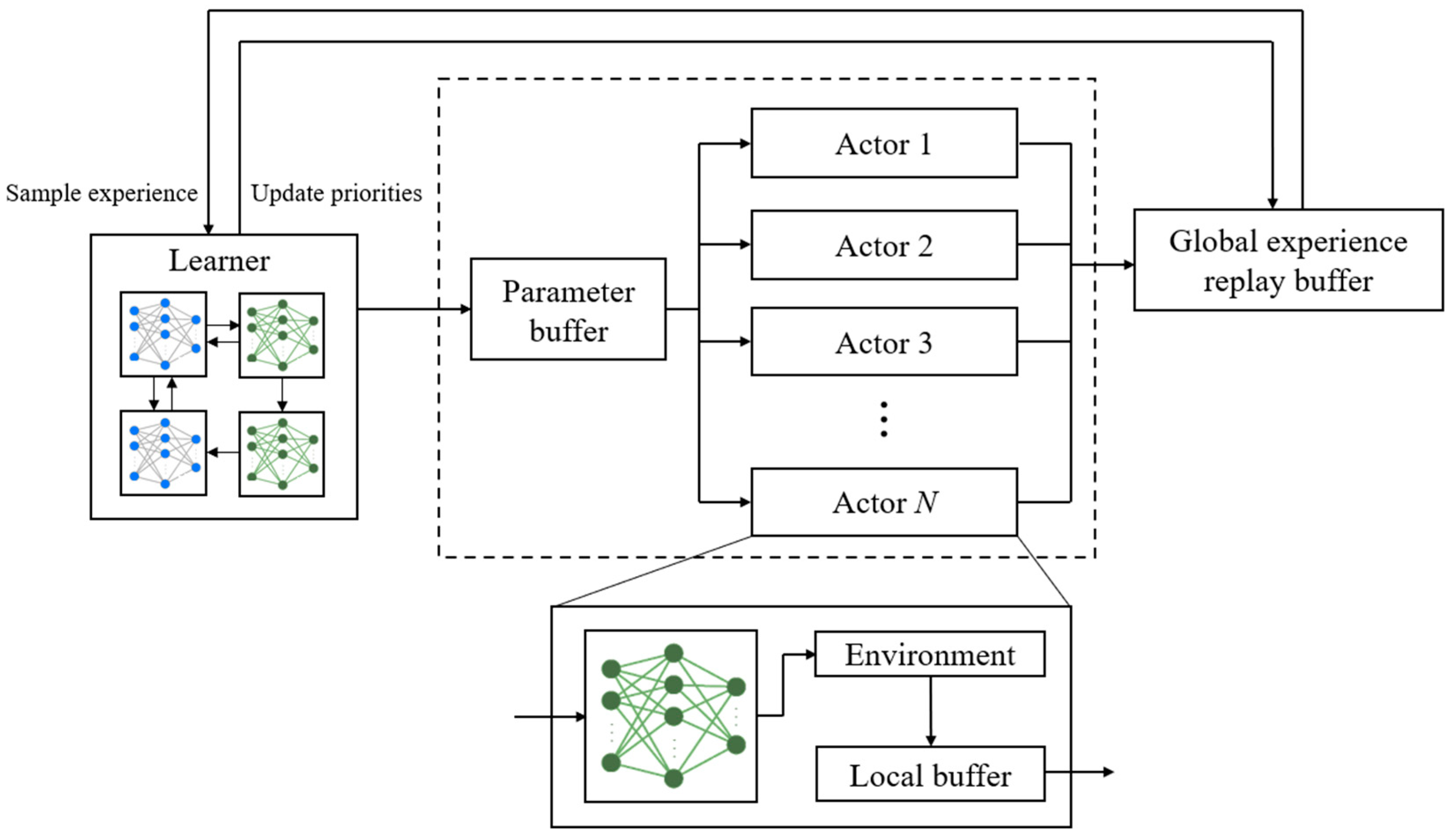
3.4. Structure of Ape-X DDPG Algorithm

The structure of the Ape-X DDPG algorithm is illustrated in Figure 5. It encompasses three components: the Learner, the Actor, and the global experience replay buffer. The Actor is responsible for collecting data samples generated during the simulation of the IRW’s steering system under the agent’s control. The Actor deploys multiple independent interaction environments using parallel, distributed computing techniques, composed of the local DDPG policy network, the local sample pool Dl, and the DIRW vehicle dynamics interaction environment. The local DDPG policy aims to enhance the guidance and steering ability of the IRWs while being controlled, which fetches the network parameters from the parameter buffer. The local sample pool serves as a cache for the experiences generated by the local Actor. When the volume of samples reaches the storage threshold Dm, these experiences are forwarded to the global experience replay buffer D.
The global experience replay buffer is dedicated to storing all samples generated during interactions. The Learner manages the actual learning process, drawing experiences from the global experience replay buffer and then updating the policy network and value network using the DDPG algorithm. After completing each training iteration, the Learner saves the trained network parameters into the parameter buffer and calculates the TD error for each sample to send to the global experience replay buffer. This TD error is used to update the sample’s priority within the shared buffer.
Ape-X DDPG parallelly executes the interaction, learning, and storage processes, achieving the decoupling of interactions and training. By deploying multiple independent Actors, the training speed and efficiency of sample collection are significantly enhanced. The algorithms of Ape-X DDPG’s Actor (Algorithm 1) and Learner (Algorithm 2) are described as follows:
Algorithm 1: Pseudocode of the Actor
Input: Initial state s0 from the environment; policy network parameters θμ from the Learner’s parameter buffer; local buffer size Dm; maximum interaction timesteps T
Output: Updated experience tuples and priorities to shared experience replay buffer D
 
01: Initialize local buffer Dl and shared experience replay buffer D.
02: Initialize state s0.
03: for t = 1 to T do
04:     Calculate action at−1 = μ(st−1; θμ).
05:     Obtain reward rt, next state st, and discount factor γt based on action at−1.
06:     Add experience tuple (st1, at−1, rt, γt) to local buffer Dl.
07:     if the size of Dl reaches Dm then
08:         Retrieve experience tuples from Dl, denoted as τl.
09:         Calculate the priority p for each experience tuple in τl.
10:         Add τl and corresponding priorities p to D.
11:     end if
12:     Periodically fetch the latest network parameters θμ from the Learner.
13: end for
14: end procedure
Algorithm 2: Pseudocode of the Learner
Input: Maximum interaction timesteps T; initial value network parameters θQ; initial policy network parameters θμ; initial shared experience replay buffer D
Output: Updated network parameters θQ and θμ
 
01: Initialize value network parameters θQ and policy network parameters θμ.
02: Send θQ and θμ to the parameter buffer shared with Actors.
03: for t = 1 to T do
04:     Sample training samples I and IS weights wi from D using PER sampling.
05:     Compute the loss function L according to Equation (21) based on I, θQ and θμ.
06:     Update the value network parameters θQ using L.
07:     Compute the policy network gradient according to Equation (22) and update θμ.
08:     Recalculate priorities p for sample I based on the TD error yi for each training sample.
09:     Update the priorities of samples in D with the newly computed priorities p.
10:     if the size of D reaches maximum capacity then
11:         Remove the experiences with the lowest priorities from D.
12:     end if
13: end for
14: end procedure

3.5. DRL-Based Controller Design

For the training process of the DIRW vehicle’s active steering controller based on DRL, the definition of the state space, action space, and reward function is very important. These directly influence the steering performance of the controller agent trained in the vehicle dynamics environment.

3.5.1. Definition of State Space

In this study, the state space S is defined as continuous and represents the vehicle dynamics data obtained through sensor observations. Specifically, the agent’s state space includes the longitudinal speed Vx of the DIRW vehicle and the kinetic variables Dx of the two IRWs of the two-axle railway vehicle. The dynamic variables Dx of IRWs include the lateral displacement and the yaw angle of the front and rear IRWs relative to the track and the difference in rotation speed between the left and right wheels of each IRW. Among them, the lateral displacement and yaw angle of the IRWs can be indirectly measured by displacement sensors arranged on the wheelsets. The difference in wheel rotation speed can be calculated from the motor encoder. Additionally, the first-order derivatives of these sensor measurements are also included in state space. Hence, the dynamic variables Dx of the two IRWs obtained through sensor observation in the state space are shown in Equation (23).
D x = y w 1 ψ w 1 ϕ ˙ w 1 y ˙ w 1 ψ ˙ w 1 ϕ ¨ w 1 y w 2 ψ w 2 ϕ ˙ w 2 y ˙ w 2 ψ ˙ w 2 ϕ ¨ w 2
Considering that the vehicle has different speeds under different running conditions, the longitudinal speed Vx of the vehicle is also one of the observations. The final state space S of the agent is represented as in Equation (24).
S = y w 1 ψ w 1 ϕ ˙ w 1 y ˙ w 1 ψ ˙ w 1 ϕ ¨ w 1 y w 2 ψ w 2 ϕ ˙ w 2 y ˙ w 2 ψ ˙ w 2 ϕ ¨ w 2 V x

3.5.2. Definition of Action Space

The active steering of IRWs is controlled through the torque of the wheel-side motors, with the DRL-based controller’s output in a continuous action space. For the DIRWs, the controller’s output separately controls the half torque difference between the left and right wheels for both the front and rear IRWs. The action space A is defined in Equation (25).
A = T w 1 T w 2
where Tw1 and Tw2 are half of the input torque difference of the left and right wheels of the front and rear IRWs, respectively, satisfying −TmaxTw1, Tw2Tmax, in which Tmax represents the maximum output torque limit of the active steering controller.
Based on the defined action space, during the operation of the DIRW vehicle, the left and right wheels of each IRW will be subjected to force torques of equal magnitude but opposite directions. The left and right wheels of the front IRW receive steering torques of Tw1 and −Tw1, respectively. Similarly, the left and right wheels of the rear IRW receive steering torques of Tw2 and −Tw2, respectively.

3.5.3. Control Objectives and Reward Function

The active steering controller of DIRW vehicles is required to meet multiple objectives. First and foremost, the controller must improve the steering stability of the IRWs. Under the guidance of the active steering controller, the IRW should avoid flange contact on both straight and curved tracks. Therefore, the controller should be designed to minimize the lateral displacement and yaw angle of the IRWs relative to the track, ensuring the steering capability of the IRWs. Based on these control objectives, in the DRL reward function, the centering performance reward of the IRW is defined as r1, as shown in Equation (26).
r 1 = η 11 y max y w 1 2 η 12 ψ w 1 2 + η 21 y max y w 2 2 η 22 ψ w 2 2
where η11, η12, η21, and η22 are the weighting coefficients for the lateral displacement and yaw angle of the two IRWs; ymax denotes the maximum lateral clearance between the wheels and rail. Since the front IRWs are more prone to losing steering capabilities, resulting in flange guidance when the vehicle runs on a curved track, the reward coefficients η11 and η12 for the front IRW are set to be greater than the weighting coefficients η21 and η22 for the rear IRW.
Furthermore, the control torque must be constrained within a reasonable range, which ensures the performance of the controller while reducing actuator output torque to improve energy efficiency. The reward function of motor output is defined as r2, as illustrated in Equation (27).
r 2 = η 13 T max T w 1 + η 23 T max T w 2
where η13 and η23 are the reward coefficients for the motor output torque.
The controller should also ensure the vehicle’s smoothness, preventing the active steering control from decreasing comfort. We measure this aspect using the vehicle’s lateral acceleration. r3 is defined as the contribution to the agent’s reward function for vehicle comfort, as shown in Equation (28). If the vehicle’s lateral acceleration exceeds a threshold, a significant penalty is applied in the reward function design.
r 3 = 0 , y ¨ b a max r p , y ¨ b > a max
where amax is the maximum allowed lateral acceleration of the vehicle under active steering control; rp is the penalty given to the agent when lateral acceleration surpasses the threshold.
In summary, the reward function is as shown in Equation (29).
r t = r 1 + r 2 + r 3
The training objective of the active steering controller is to maximize the designed reward function rt, ensuring the controlled IRWs reduce the lateral displacement and attack angle and restore the running stability. Simultaneously, the agent should learn to decrease control torque while achieving the desired control effects.

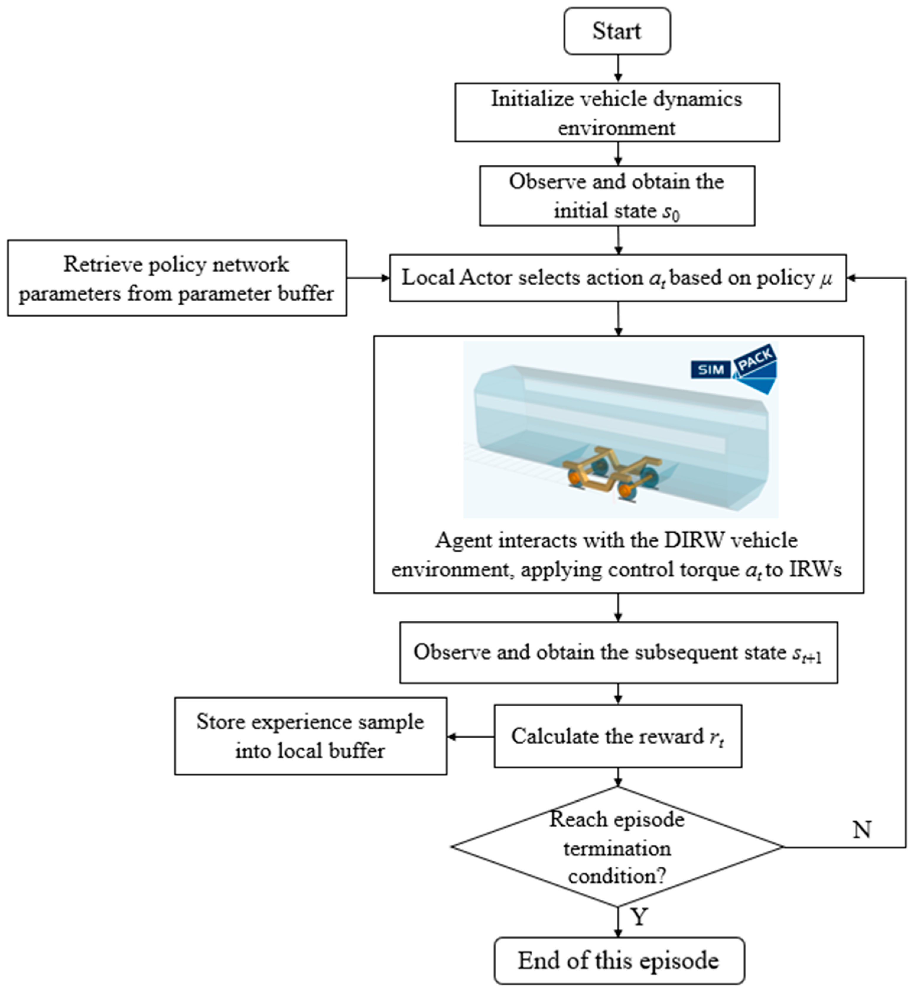
3.5.4. DRL Interaction and Training Process

Within our Ape-X DDPG training framework, the neural network parameters for the policy network (actor network) and value network (critic network) are initialized randomly. For storing experience tuples, a shared experience replay buffer needs also to be initialized. We set up N parallel Actors that perform action sampling in the environment based on the current policy. Each episode has a maximum time step of 20 s, during which experience tuples are collected and stored in their respective local experience buffers.
During the data collection phase, each episode’s training process for every Actor is shown in Figure 6. Inside each Actor unit, the active steering controller agent calculates actions based on the policy network. This action, representing half of the torque difference between the left and right wheels for both the front and rear IRWs, is applied accordingly. According to the dynamic response of the DIRW vehicle, the observation for the next time step is obtained as the next state, and the corresponding reward is also calculated. The agent’s control frequency is 100 Hz, meaning that every 0.01 s, the IRW will receive active steering torque from the agent. During the DRL controller’s training process, the interaction between the agent and the environment will be terminated, and the environment state will be reinitialized if any of the following four situations occur:
(a)
The training episode reaches the maximum timestep T.
(b)
The lateral displacement of the IRWs reaches the maximum wheel–rail clearance.
(c)
The control torque output from the policy network exceeds the maximum limit.
(d)
Under the effect of the active steering controller, the lateral acceleration of the vehicle body exceeds the threshold.
To enhance the adaptability of the agent under different vehicle operating conditions, every time the vehicle dynamics environment is initialized, the longitudinal speed, curve radius, and superelevation of the vehicle’s operation are reset. The training conditions for each episode are randomly selected from five different operating speeds and curve radii. The operating conditions for the DIRW vehicle are shown in Table 1.
Experience tuples generated from the interaction between the agent and the vehicle dynamics environment are stored in their respective local experience buffers. When the local buffer reaches the storage threshold, experiences are batched and sent to the global shared experience replay buffer. At the same time, the Actor periodically retrieves the latest policy network parameters from the Learner.
During the model training phase, the Learner prioritizes sampling from the global experience replay buffer and extracts training samples to calculate the loss function. This is used to update the parameters of the value network and to update the policy network parameters using the gradient of the policy network. After updating the value network, the TD error for each sample is recalculated to update the priority of the samples in the global experience replay buffer. The training process is repeated continuously, enabling the continuous optimization of the policy network and value network until the model’s performance converges.

4. Training and Simulation Results

4.1. Training Environment

This paper conducts co-simulation through the multibody dynamics simulation software SIMPACK and the Python-based reinforcement learning framework RLlib [33,34] to validate the learning and control capabilities of the Ape-X DDPG active steering controller. Specifically, RLlib is responsible for implementing Ape-X DDPG, while SIMPACK handles the dynamics simulation for the DIRW two-axle railway vehicle. The SIMPACK Realtime API facilitates data communication between SIMPACK and RLlib. In SIMPACK, the parameters for the two-axle DIRW railway vehicle dynamics model are shown in Table A1, and the UIC60 rail profile and S1002 wheel profile are used. The contact tangential forces are calculated using the FASTSIM method. The state values and rewards required for DRL training are calculated by SIMPACK and transferred to RLlib at each time step.
All DRL training was conducted on a server running Ubuntu 20.04, equipped with dual Intel Gold 6132 CPUs, clocked at 2.60 GHz, and an NVIDIA GeForce RTX 2080 Ti GPU used for deep learning computations. In RLlib, the Ape-X DDPG algorithm is implemented using Pytorch [35]. Heterogeneous training is adopted, with Actors interacting with the vehicle dynamics environment distributed across different CPU cores for parallel computing. In contrast, the Learner is assigned to the GPU for neural network gradient descent optimization. In the Learner unit, both the policy network μ and the value network Q use fully connected deep neural networks, each with four hidden layers. The unit counts for these layers are 200, 400, 400, and 50. ReLU is chosen as the activation function for the hidden layers, with Adam [36] being used as the optimizer for the neural network parameters. The input layer network unit count is determined by the state space, and Q receives the corresponding action in the second hidden layer. For the output layer activation function, both μ and Q use the tanh activation function. Detailed DRL neural network training parameters are presented in Table 2.

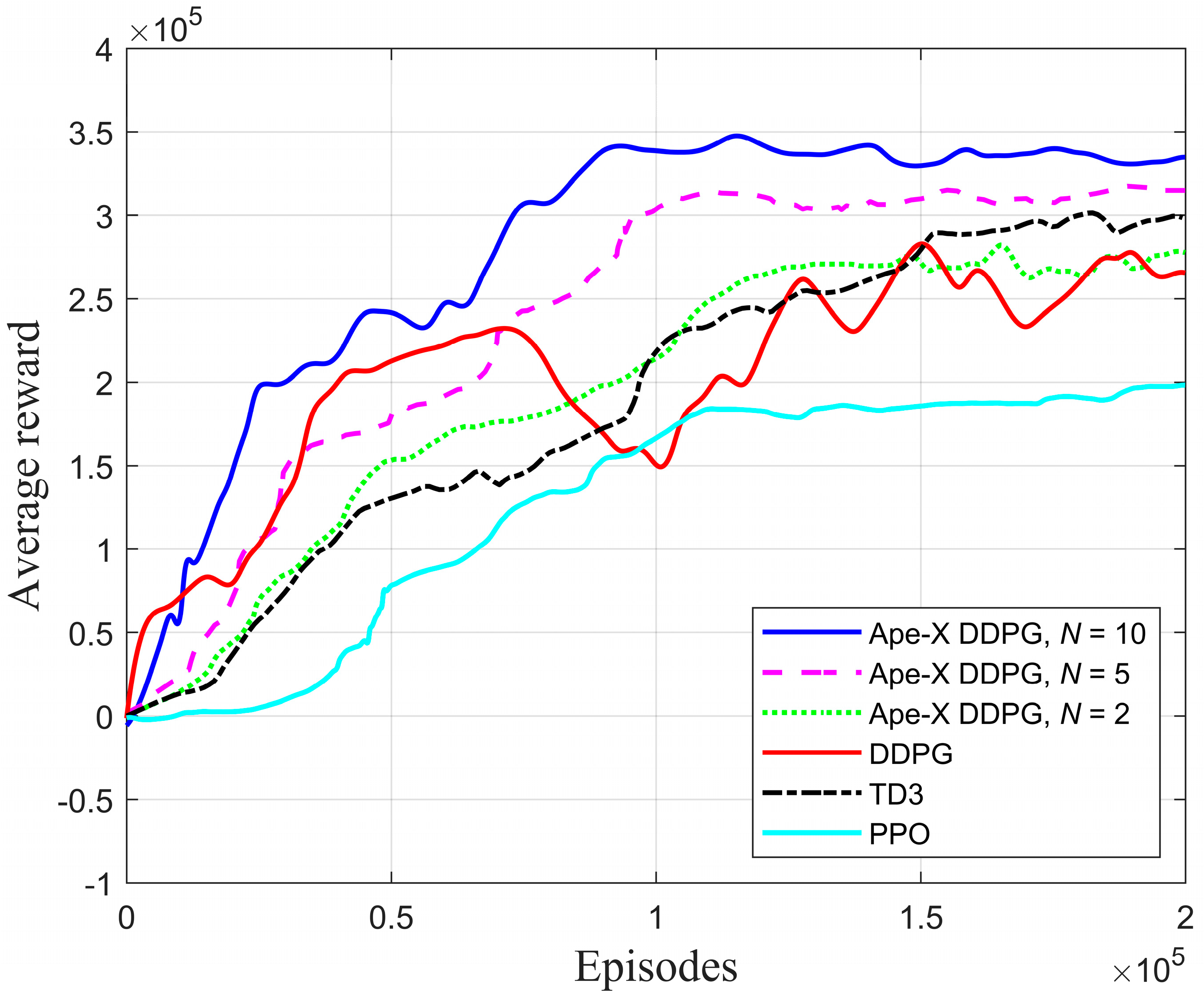
4.2. Training Comparison of DRL

A comparative experiment was conducted to evaluate the influence of the number of Actors in Ape-X DDPG on its performance and to compare it against other DRL algorithms, such as DDPG, Proximal Policy Optimization (PPO), and Twin Delayed DDPG (TD3). In our experimental setup, PPO employs mini-batches of size 64, and TD3 uses a policy delay setting of 2. PPO aims to stabilize the training process by optimizing a surrogate objective function and limiting policy updates, as referenced in [37]. TD3, an extension of DDPG, uses dual value function networks to improve bootstrapping accuracy and introduces delayed policy updates to reduce estimation errors [38].
The impact of the number of Actors in Ape-X DDPG is significant. Therefore, we conducted simulation experiments with three different numbers of Actors—2, 5, and 10—to investigate their effects on learning efficiency and convergence speed. We measured the performance of each DRL algorithm through their respective reward curves after 2 × 10⁵ training episodes, as shown in Figure 7.
Our results indicate that the average reward values after convergence for the Ape-X DDPG configurations are positively correlated with the number of Actors (N). Ape-X DDPG, a distributed version of DDPG, particularly excels when N is set to 5 or 10. In contrast, standard DDPG shows a slower learning curve and oscillations, achieving lower final rewards than Ape-X DDPG when N = 10. Ape-X DDPG not only converges more quickly but also demonstrates enhanced stability during training, leading to higher final rewards. While TD3 improves upon DDPG, it still does not outperform Ape-X DDPG when N is 5 or 10.
To test the robustness of these DRL algorithms, we conducted further experiments with 1000 randomly sampled groups from the initial state space. Each DRL algorithm used network parameters obtained from previous training. The test evaluated the ability of these algorithms to complete 20 s of active steering under various operating conditions for DIRW vehicles. Figure 8 plots the number of successful episodes for each controller.
In Figure 8, DDPG and Ape-X DDPG with two Actors show similar performance, while TD3 outperforms both. However, Ape-X DDPG with 10 Actors achieves the best performance, successfully completing 961 active steering episodes under various initial operating conditions without triggering early termination.
In summary, the Ape-X DDPG algorithm, particularly when configured with 10 Actors, exhibits marked superiority over other DRL algorithms like DDPG, PPO, and TD3 in terms of active steering control. It not only converges faster but also achieves higher final rewards. Furthermore, it demonstrates robust performance under various initial conditions. Therefore, Ape-X DDPG with 10 Actors will be the chosen algorithm for comparative studies in subsequent simulation experiments.

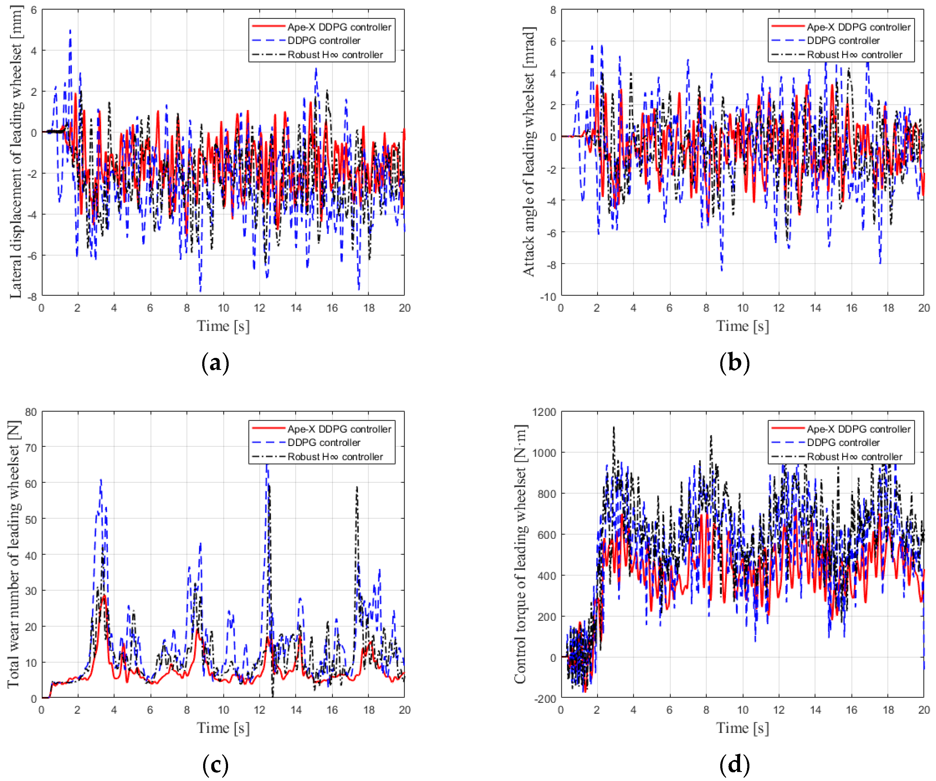
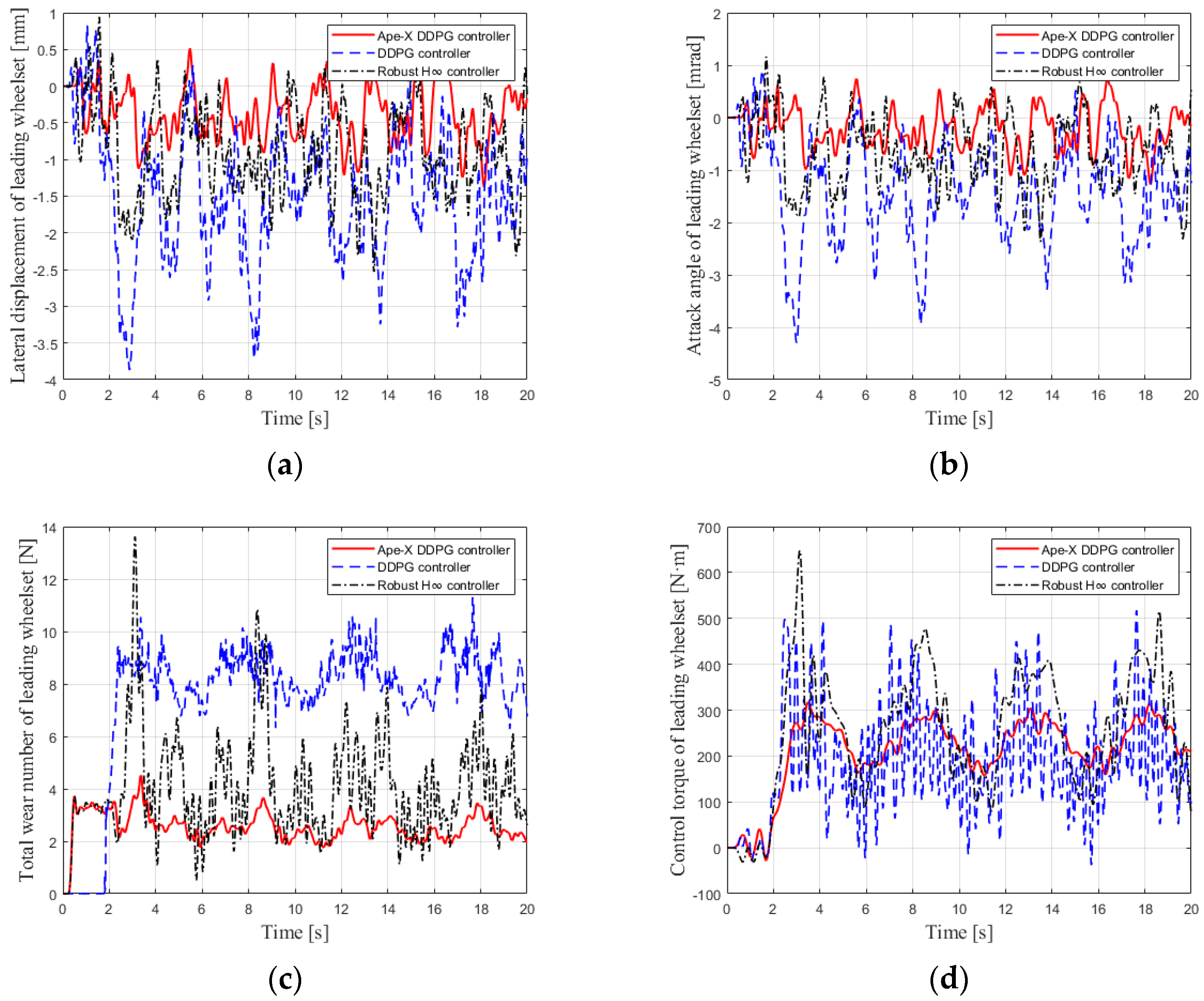
4.3. Comparative Analysis of Control Effects between Model-Based and Data-Based Algorithms

To validate the improvement in centering performance and curve steering ability of the DIRW vehicle by the Ape-X DDPG active controller, this study selected the data-driven classic DDPG algorithm and the model-based robust H∞ control [14] algorithm for comparison with our proposed Ape-X DDPG controller. The robust H∞ control, rooted in the μ-synthesis [39] method, is designed for MIMO systems characterized by uncertainties. In the design of the DIRW vehicle dynamics controller, wheel–rail creep contact and wheel conicity are considered as uncertainty parameters that vary within a certain range. Leveraging this robust H∞ control approach, an adaptive controller robust to the ever-changing wheel–rail contact dynamic characteristics is developed, relying on the D-K iteration process.
Three typical DIRW vehicle operating conditions from Table 1 were selected for detailed analysis. Given that leading IRW often plays a more critical guiding role than the rear IRW, the lateral displacement and yaw angle of the front IRW during curve running are generally significantly greater than those of the rear IRW. Therefore, in each operating condition, we compared the lateral displacement and yaw angle, wear number, and received steering control torque of the front IRW during running.
(1)
Case 1: Operation on a straight track at 120 km/h.
The simulation results for Case 1 are shown in Figure 9. For the leading IRW wheelset, all three control algorithms avoid flange contact to prevent severe wheel–rail wear. Under the guidance of the Ape-X DDPG active steering controller, the maximum lateral displacement of the wheelset is 4.4 mm. In comparison to the 9.1 mm with the DDPG controller and 8.2 mm with the H∞ control controller, it demonstrates significant advantages in centering performance. With the controller proposed in this paper, the maximum attack angle of the front IRW under this operating condition is only 2.2 mrad. For comparison, the maximum wheelset attack angle under DDPG control is 5.5 mrad, and it is 4.6 mrad under H∞ control.
The fundamental purpose of active steering control is to reduce wear between the wheel and the rail. The simulation results indicate that by applying the active steering control proposed in this paper, the average wear number of the wheelset drops from 8.5 N under the DDPG controller and 4.6 N under the H∞ controller to 2.5 N. This means that Ape-X DDPG reduces wheel–rail wear by 71% and 46%, respectively, compared to the other two controllers. The maximum output torque of the Ape-X DDPG controller is 178 N·m, which is lower than the other controllers, indicating that the control torque adequately meets the design requirements.
(2)
Case 2: Operation on a curved track with Rc = 70 m at 30 km/h.
The simulation results for Case 2 are shown in Figure 10. The results indicate that, in the case of a small curved line, the controller still maintains good curve guidance capability, avoiding wheel flange guidance and reducing wheel–rail wear. Under the Ape-X DDPG controller, the maximum lateral displacement of the leading wheelset is 5.1 mm, and the attack angle is 5.4 mrad. This is less than the 7.8 mm/8.5 mrad under the DDPG controller and 6.4 mm/6.5 mrad under the H∞ controller. The average wear number of our proposed controller on a small-radius curve is only 8.7 N, which is a 54% reduction compared to the DDPG controller and a 37% reduction compared to the H∞ controller. The maximum wear number is 28.6 N, which is less than the other two controllers used for comparison. The Ape-X DDPG controller has a maximum output torque of 725 N·m and an average torque of 431 N·m, reducing the requirements for control output peaks and control bandwidth compared to the other two controllers.
(3)
Case 3: Operation on a curved track with Rc = 250 m at 80 km/h.
The simulation results for Case 3 are shown in Figure 11. Due to the increase in curve radius, the control effect is better relative to Case 2. The Ape-X DDPG controller allows the IRW to stay almost radially positioned, with both the front wheelset’s lateral displacement and attack angle kept at low levels. The maximum lateral displacement is 1.37 mm, and the maximum attack angle is 1.3 mrad. These values are superior to the 3.9 mm/4.3 mrad of the DDPG controller and the 2.5 mm/2.4 mrad of the H∞ controller. The total wear number remains at a low value, with an average wear number of 2.6 N for our proposed controller. The peak control torque is 318 N·m, only a small fraction of the motor’s maximum output torque. Additionally, thanks to the improved experience replay strategy, the output of the Ape-X DDPG controller is smoother than that of the DDPG controller.
Comparing the control effects of different controllers under various conditions, the Ape-X DDPG controller significantly improves the IRW’s straight-track centering performance and curve steering capability and can greatly reduce wheel–rail wear. At the same time, the controller’s output torque is stable and less than the motor’s peak torque.

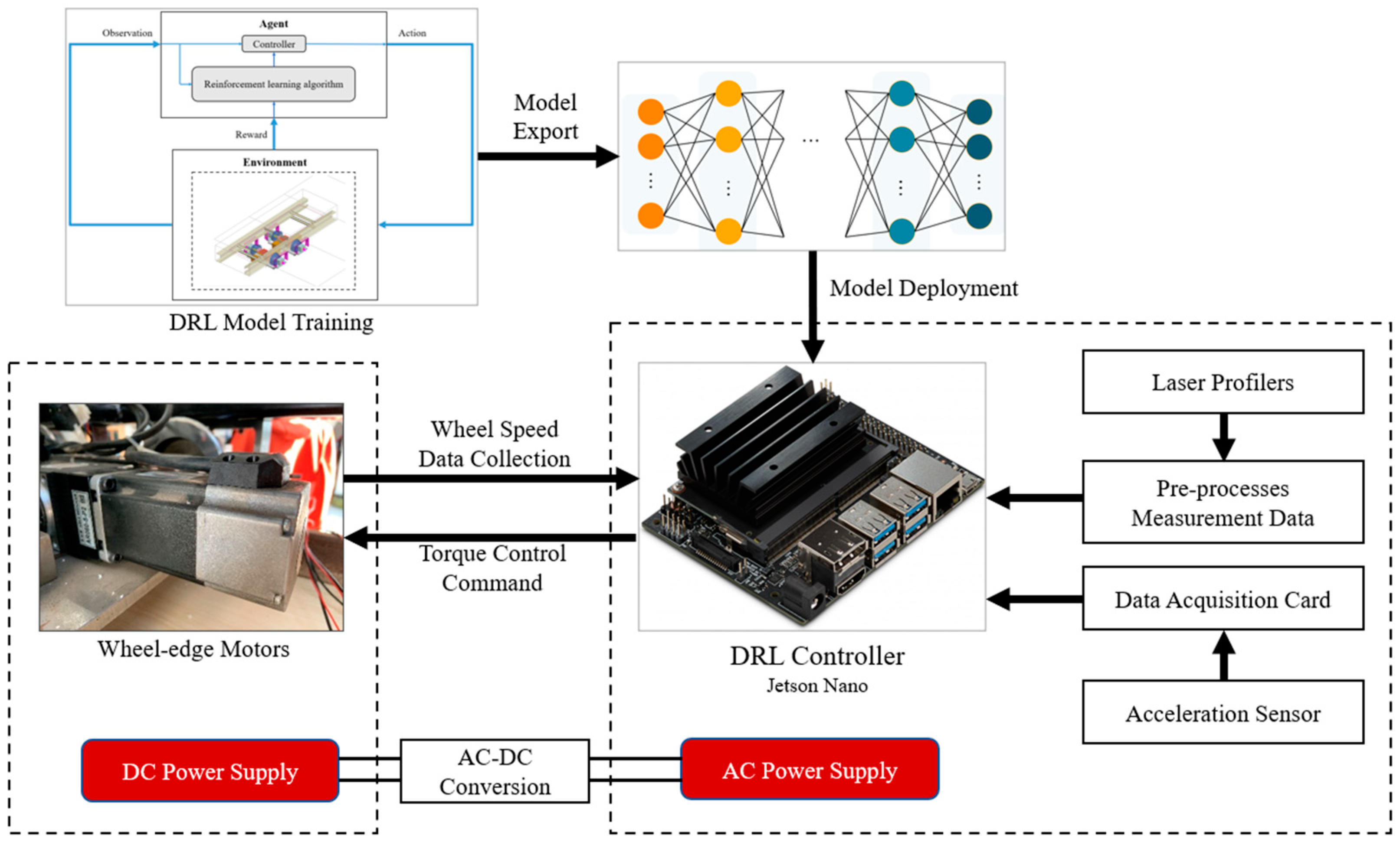
5. Scale Model Experiments

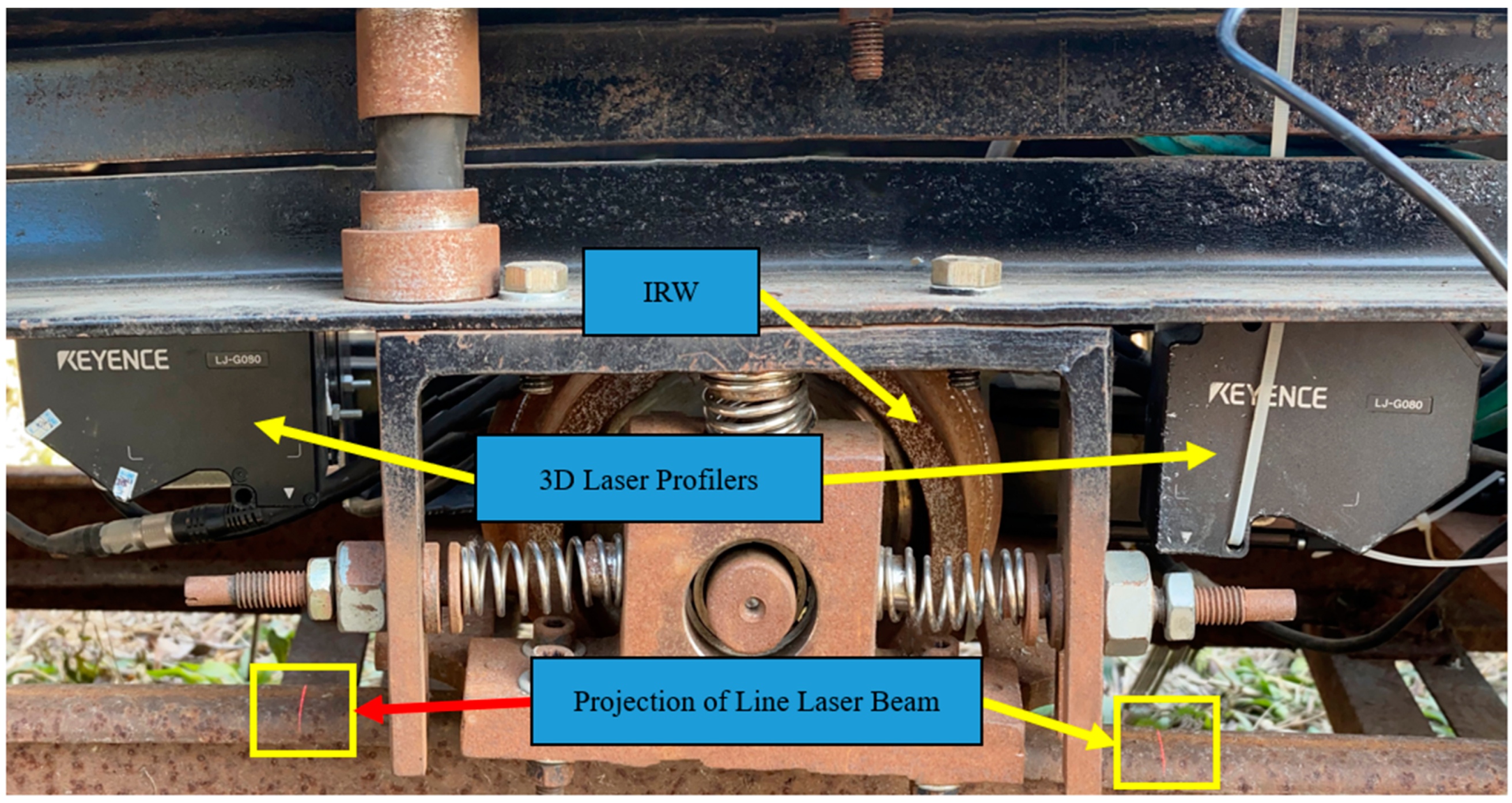
5.1. Scale DIRW Vehicle

To verify the performance of the Ape-X DDPG controller in a real vehicle operating environment, we designed and manufactured a 1:5 scale IRW model for experimental verification, as shown in Figure 12. The DRL-based controller is trained using the digital twin dynamics model of the scaled DIRW vehicle and is deployed on the test vehicle. This scaled model comprises a bogie and a carbody and two subframes, each equipped with IRWs. The primary and secondary suspensions are steel springs and rubber bushings, respectively, and they support the mass of the upper carbody. The left and right wheels are connected to the reduction gearboxes via short axles. Four 600 W servo motors transfer the active steering control torque to the IRWs through the reduction gearboxes. Each drive system and IRW are located on the same subframe, ensuring synchronized movement in lateral, yaw, and other directions.
The block diagram of the scaled model’s control system is shown in Figure 13.
The scaled model is powered by an AC source, converting the input voltage into a three-phase AC high-voltage circuit for the drive motor via an inverter, as well as a low-voltage for the controller and sensors. The active steering controller’s hardware is based on the NVIDIA Jetson Nano edge computing development board. Once the controller is trained using reinforcement learning algorithms, it is exported in the Open Neural Network Exchange (ONNX) format, which contains the neural network structure and weight parameters. This exported model is subsequently transformed into CUDA executable code using TensorRT and is then deployed on the Jetson Nano.

5.2. Acquisition of Sensor Signals

The wheel–rail relative position needed by the active steering controller, including the lateral displacement and yaw angle of the IRW relative to the track, is obtained through laser profilers mounted on each IRW. Compared to point laser displacement sensors and eddy current displacement sensors, the laser profilers offer a broader measurement range and higher accuracy. Even when there is significant lateral displacement and attack angle between the wheel and rail, the laser profilers can still ensure the measurement beam projects on the rail surface, avoiding the loss of reflected laser measurement points which could lead to control failure.
The laser profilers are mounted on the subframes, located both at the front and back of each IRW, with the laser emitting vertically downwards towards the top of the rail, as depicted in Figure 14. Each set of laser profilers obtains the two-dimensional coordinates of the rail’s outer contour during vehicle operation. By fitting these coordinates with a quartic curve and comparing the peak coordinates of the contour to the baseline (when the lateral displacement is zero), the current lateral displacement between the laser profiler and rail can be calculated.
The wheelset’s lateral displacement and yaw angle can be calculated using Equations (30) and (31).
y w i = y s 1 , i + y s 2 , i 2
ψ w i = y s 1 , i y s 2 , i L s
where ys1,i and ys2,i are the lateral displacement values of the two sets of laser profilers at each IRW, with subscript i = 1,2 indicating the front and rear IRWs, respectively. Ls represents the longitudinal interval distance between the two sets of laser profilers at each IRW.

5.3. Experimental Results

The active control experiment of the DIRW scaled model was conducted on a 1:5 railway test track, which includes a 10 m straight track and a 10 m curved track with a radius of 15 m. The vehicle runs through the test track at a speed of 2 m/s, and each experiment of the scaled model lasts for 10 s. We deployed four control methods: passive travel, H∞ control, DDPG controller, and Ape-X DDPG controller.
The experimental results of the scaled model are shown in Figure 15, displaying data for the front IRW’s lateral displacement, yaw angle, and steering torque. Without active steering control in the IRW, the maximum lateral displacement was 6.9 mm on the straight track and 9.8 mm on the curved track due to wheel flange guiding, causing intense wheel–rail wear. Using the Ape-X DDPG controller proposed in this paper, the lateral displacement of the IRW can be controlled within ±0.5 mm on the straight track and ±2 mm on the curved track. The maximum control torque occurred at the transition of the curve and straight track, at 5.3 N·m, which is below the motor’s peak output torque. Relatively speaking, both the DDPG-based controller and the H∞-based controller had greater maximum lateral displacements and attack angles during operation compared to our proposed controller. Additionally, the Ape-X DDPG controller responds smoothly, reducing the dynamic response requirements for the motor. Therefore, we conclude that the Ape-X DDPG controller effectively meets the design requirements.

6. Conclusions

This study introduced an active steering controller for DIRW vehicles based on the DRL algorithm, effectively enhancing the guidance capability of IRWs and reducing wheel–rail wear. Given the complex wheel–rail contact dynamics in the railway vehicle system, traditional design methodologies struggle to effectively design controllers for highly nonlinear systems. However, reinforcement learning, through constant trial and error and maximizing the reward function, combined with the deep neural network’s capability to fit nonlinear systems, allows the controller to adaptively train and attain optimal strategies. We integrated DPER with the DDPG algorithm in our DRL controller’s training and interaction, leading to the implementation of the Ape-X DDPG algorithm. This was to address the classic DDPG algorithm’s challenges, such as low sample efficiency and propensity to get stuck in local optima. Using the multibody dynamics theory, we established a nonlinear DIRW vehicle model and trained the Ape-X DDPG controller, and the control efficacy was validated under multiple vehicle operational conditions. Both simulation results and scaled model experiments demonstrate that our control strategy outperforms previous methods. With the intervention of the Ape-X DDPG active guidance controller, the IRWs have enhanced straight-line centering performance and curve guidance ability while diminishing wheel–rail wear. This research underscores the significance of DRL-based controllers in terms of efficacy and feasibility when the large-scale application of DIRW’s active steering control is considered.

Author Contributions

Conceptualization, Z.L.; Methodology, Z.L.; Validation, Z.L.; Formal analysis, J.W.; Investigation, J.W.; Resources, Z.W.; Data curation, Z.W.; Writing—original draft, Z.L.; Writing—review & editing, J.W. and Z.W. All authors have read and agreed to the published version of the manuscript.

Funding

This research received no external funding.

Data Availability Statement

The data that support the findings of this study are available from the corresponding author upon reasonable request.

Conflicts of Interest

The authors declare no conflict of interest.

Appendix A

Table A1. Parameters of the DIRW vehicle.
Dynamic ParametersValueUnit
Wheel base2.0m
Lateral length of primary suspension1.08m
Longitudinal length of primary suspension0.39m
Lateral length of secondary suspension1.80m
Longitudinal length of secondary suspension0.50m
Mass of carbody9000kg
Pitch moment of inertia of carbody80,000kg·m2
Yaw moment of inertia of carbody80,000kg·m2
Roll moment of inertia of carbody10,000kg·m2
Mass of bogie1600kg
Pitch moment of inertia of bogie900kg·m2
Yaw moment of inertia of bogie1300kg·m2
Roll moment of inertia of bogie1500kg·m2
Mass of IRW1250kg
Pitch moment of inertia per wheel30kg·m2
Yaw moment of inertia of IRW600kg·m2
Primary longitudinal stiffness per axle box600kN·m−1
Primary lateral stiffness per axle box8000kN·m−1
Primary vertical stiffness per axle box15,000kN·m−1
Primary longitudinal damping per axle box100kN·m·s−1
Primary lateral damping per axle box500kN·m·s−1
Primary vertical damping per axle box800kN·m·s−1
Secondary longitudinal stiffness per side200kN·m−1
Secondary lateral stiffness per side200kN·m−1
Secondary vertical stiffness per side600kN·m−1
Secondary longitudinal damping side50kN·m·s−1
Secondary lateral damping per side50kN·m·s−1
Secondary vertical damping per side50kN·m·s−1

References

  1. Fu, B.; Giossi, R.L.; Persson, R.; Stichel, S.; Bruni, S.; Goodall, R. Active suspension in railway vehicles: A literature survey. Railw. Eng. Sci. 2020, 28, 3–35. [Google Scholar] [CrossRef]
  2. Goodall, R.; Mei, T.X. Mechatronic strategies for controlling railway wheelsets with independently rotating wheels. In Proceedings of the 2001 IEEE/ASME International Conference on Advanced Intelligent Mechatronics, Proceedings (Cat. No.01TH8556), Como, Italy, 8–12 July 2001; Volume 1, pp. 225–230. [Google Scholar]
  3. Oh, Y.J.; Liu, H.-C.; Cho, S.; Won, J.H.; Lee, H.; Lee, J. Design, modeling, and analysis of a railway traction motor with independently rotating wheelsets. IEEE Trans. Magn. 2018, 54, 8205305. [Google Scholar] [CrossRef]
  4. Pérez, J.; Busturia, J.M.; Mei, T.X.; Vinolas, J. Combined active steering and traction for mechatronic bogie vehicles with independently rotating wheels. Annu. Rev. Control 2004, 28, 207–217. [Google Scholar] [CrossRef]
  5. Mei, T.X.; Li, H.; Goodall, R.M.; Wickens, A.H. Dynamics and control assessment of rail vehicles using permanent magnet wheel motors. Veh. Syst. Dyn. 2002, 37 (Suppl. 1), 326–337. [Google Scholar] [CrossRef]
  6. Chudzikiewicz, A.; Gerlici, J.; Sowinska, M.; Sowinska, M.; Stelmach AWawrzyński, W. Modeling and simulation of a control system of wheels of wheelset. Arch. Transp. 2020, 55, 73–83. [Google Scholar] [CrossRef]
  7. Ji, Y.; Ren, L.; Zhou, J. Boundary conditions of active steering control of independent rotating wheelset based on hub motor and wheel rotating speed difference feedback. Veh. Syst. Dyn. 2018, 56, 1883–1898. [Google Scholar] [CrossRef]
  8. Mei, T.X.; Qu, K.W.; Li, H. Control of wheel motors for the provision of traction and steering of railway vehicles. IET Power Electron. 2014, 7, 2279–2287. [Google Scholar] [CrossRef]
  9. Heckmann, A.; Schwarz, C.; Keck, A.; Bünte, T. Nonlinear observer design for guidance and traction of railway vehicles. In Advances in Dynamics of Vehicles on Roads and Tracks: Proceedings of the 26th Symposium of the International Association of Vehicle System Dynamics, IAVSD 2019, Gothenburg, Sweden, 12–16 August 2019; Springer International Publishing: Cham, Switzerland, 2020. [Google Scholar]
  10. Ahn, H.; Lee, H.; Go, S.; Cho, Y.; Lee, J. Control of the lateral displacement restoring force of IRWs for sharp curved driving. J. Electr. Eng. Technol. 2016, 11, 1042–1048. [Google Scholar] [CrossRef]
  11. Liu, X.; Goodall, R.; Iwnicki, S. Active control of independently-rotating wheels with gyroscopes and tachometers–simple solutions for perfect curving and high stability performance. Veh. Syst. Dyn. 2021, 59, 1719–1734. [Google Scholar] [CrossRef]
  12. Kurzeck, B.; Heckmann, A.; Wesseler, C.; Rapp, M. Mechatronic track guidance on disturbed track: The trade-off between actuator performance and wheel wear. Veh. Syst. Dyn. 2014, 52 (Suppl. 1), 109–124. [Google Scholar] [CrossRef]
  13. Grether, G. Dynamics of a running gear with IRWs on curved tracks for a robust control development. PAMM 2017, 17, 797–798. [Google Scholar] [CrossRef]
  14. Lu, Z.; Yang, Z.; Huang, Q.; Wang, X. Robust active guidance control using the µ-synthesis method for a tramcar with independently rotating wheelsets. Proc. Inst. Mech. Eng. Part F J. Rail Rapid Transit 2019, 233, 33–48. [Google Scholar] [CrossRef]
  15. Yang, Z.; Lu, Z.; Sun, X.; Zou, J.; Wan, H.; Yang, M.; Zhang, H. Robust LPV-H∞ control for active steering of tram with independently rotating wheels. Adv. Mech. Eng. 2022, 14, 16878132221130574. [Google Scholar] [CrossRef]
  16. Lu, Z.; Sun, X.; Yang, J. Integrated active control of independently rotating wheels on rail vehicles via observers. Proc. Inst. Mech. Eng. Part F J. Rail Rapid Transit 2017, 231, 295–305. [Google Scholar] [CrossRef]
  17. Wei, J.; Lu, Z.; Yang, Z.; He, Y.; Wang, X. Data-Driven Robust Control for Railway Driven Independently Rotating Wheelsets Using Deep Deterministic Policy Gradient. In Proceedings of the IAVSD International Symposium on Dynamics of Vehicles on Roads and Tracks, Saint Petersburg, Russia, 17–19 August 2021; Springer International Publishing: Cham, Switzerland, 2021. [Google Scholar]
  18. Ramos-Fernández, J.C.; López-Morales, V.; Márquez-Vera, M.A.; Pérez JM, X.; Suarez-Cansino, J. Neuro-fuzzy modelling and stable PD controller for angular position in steering systems. Int. J. Automot. Technol. 2021, 22, 1495–1503. [Google Scholar] [CrossRef]
  19. Mei, T.X.; Goodall, R.M. Robust control for independently rotating wheelsets on a railway vehicle using practical sensors. IEEE Trans. Control. Syst. Technol. 2001, 9, 599–607. [Google Scholar] [CrossRef]
  20. Sutton, R.S.; Barto, A.G. Reinforcement Learning: An Introduction; MIT Press: Cambridge, MA, USA, 2018; p. 342. [Google Scholar]
  21. Deng, H.; Zhao, Y.; Nguyen, A.T.; Huang, C. Fault-tolerant predictive control with deep-reinforcement-learning-based torque distribution for four in-wheel motor drive electric vehicles. IEEE/ASME Trans. Mechatron. 2023, 28, 668–680. [Google Scholar] [CrossRef]
  22. Wei, H.; Zhao, W.; Ai, Q.; Zhang, Y.; Huang, T. Deep reinforcement learning based active safety control for distributed drive electric vehicles. IET Intell. Transp. Syst. 2022, 16, 813–824. [Google Scholar] [CrossRef]
  23. Albarella, N.; Lui, D.G.; Petrillo, A.; Santini, S. A Hybrid Deep Reinforcement Learning and Optimal Control Architecture for Autonomous Highway Driving. Energies 2023, 16, 3490. [Google Scholar] [CrossRef]
  24. Cheng, Y.; Hu, X.; Chen, K.; Yu, X.; Luo, Y. Online longitudinal trajectory planning for connected and autonomous vehicles in mixed traffic flow with deep reinforcement learning approach. J. Intell. Transp. Syst. 2023, 27, 396–410. [Google Scholar] [CrossRef]
  25. Wang, H.; Han, Z.; Liu, Z.; Wu, Y. Deep reinforcement learning based active pantograph control strategy in high-speed railway. IEEE Trans. Veh. Technol. 2022, 72, 227–238. [Google Scholar] [CrossRef]
  26. Zhu, F.; Yang, Z.; Lin, F.; Xin, Y. Decentralized cooperative control of multiple energy storage systems in urban railway based on multiagent deep reinforcement learning. IEEE Trans. Power Electron. 2020, 35, 9368–9379. [Google Scholar] [CrossRef]
  27. Sresakoolchai, J.; Kaewunruen, S. Railway infrastructure maintenance efficiency improvement using deep reinforcement learning integrated with digital twin based on track geometry and component defects. Sci. Rep. 2023, 13, 2439. [Google Scholar] [CrossRef]
  28. Farazi, N.P.; Zou, B.; Ahamed, T.; Barua, L. Deep reinforcement learning in transportation research: A review. Transp. Res. Interdiscip. Perspect. 2021, 11, 100425. [Google Scholar]
  29. Lee, M.F.R.; Yusuf, S.H. Mobile robot navigation using deep reinforcement learning. Processes 2022, 10, 2748. [Google Scholar] [CrossRef]
  30. Moriya, N.; Shigemune, H.; Sawada, H. A robotic wheel locally transforming its diameters and the reinforcement learning for robust locomotion. Int. J. Mechatron. Autom. 2022, 9, 22–31. [Google Scholar] [CrossRef]
  31. Li, Y. Deep reinforcement learning: An overview. arXiv 2017, arXiv:1701.07274. [Google Scholar]
  32. Lillicrap, T.P.; Hunt, J.J.; Pritzel, A.; Heess, N.; Erez, T.; Tassa, Y.; Silver, D.; Wierstra, D. Continuous control with deep reinforcement learning. arXiv 2015, arXiv:1509.02971. [Google Scholar]
  33. Moritz, P.; Nishihara, R.; Wang, S.; Tumanov, A.; Liaw, R.; Liang, E.; Elibol, M.; Yang, Z.; Paul, W.; Jordan, M.I.; et al. Ray: A distributed framework for emerging AI applications. In Proceedings of the 13th USENIX Symposium on Operating Systems Design and Implementation (OSDI 18), Carlsbad, CA, USA, 8–10 October 2018. [Google Scholar]
  34. Liang, E.; Liaw, R.; Nishihara, R.; Moritz, P.; Fox, R.; Goldberg, K.; Gonzalez, J.; Jordan, M.; Stoica, I. RLlib: Abstractions for distributed reinforcement learning. In Proceedings of the 35th International Conference on Machine Learning, Stockholm, Sweden, 10–15 July 2018. [Google Scholar]
  35. Paszke, A.; Gross, S.; Massa, F.; Lerer, A.; Bradbury, J.; Chanan, G.; Killeen, T.; Lin, Z.; Gimelshein, N.; Antiga, L.; et al. Pytorch: An imperative style, high-performance deep learning library. In Proceedings of the 33rd Conference on Neural Information Processing Systems (NeurIPS 2019), Vancouver, BC, Canada, 8–14 December 2019; Volume 32. [Google Scholar]
  36. Kingma, D.P.; Jimmy, B. Adam: A method for stochastic optimization. arXiv 2014, arXiv:1412.6980. [Google Scholar]
  37. Schulman, J.; Wolski, F.; Dhariwal, P.; Radford, A.; Klimov, O. Proximal policy optimization algorithms. arXiv 2017, arXiv:1707.06347. [Google Scholar]
  38. Fujimoto, S.; Hoof, H.; Meger, D. Addressing function approximation error in actor-critic methods. In Proceedings of the International Conference on Machine Learning, Stockholm, Sweden, 10–15 July 2018. [Google Scholar]
  39. Skogestad, S.; Postlethwaite, I. Multivariable feedback control: Analysis and design. In Multivariable Feedback Control: Analysis and Design, 2nd ed.; John Wiley & Sons: Hoboken, NJ, USA, 2005. [Google Scholar]
Figure 1. Structure of the DIRW vehicle.
Processes 11 02677 g001
Figure 2. Lateral dynamics model.
Processes 11 02677 g002
Figure 3. The overview of the DRL-based method.
Processes 11 02677 g003
Figure 4. The DDPG algorithm structure framework.
Processes 11 02677 g004
Figure 5. Ape-X DDPG algorithm structure.
Processes 11 02677 g005
Figure 6. Interaction process of Actors for each episode.
Processes 11 02677 g006
Figure 7. Average reward value vs. episodes.
Processes 11 02677 g007
Figure 8. Number of completed episodes by each DRL algorithm in the test set.
Processes 11 02677 g008
Figure 9. Case 1 simulation results (straight track, Vx = 120 km/h). (a) Lateral displacement. (b) Attack angle. (c) Wear number. (d) Control torque.
Processes 11 02677 g009
Figure 10. Case 2 simulation results (curved track with Rc = 70 m, Vx = 30 km/h). (a) Lateral displacement. (b) Attack angle. (c) Wear number. (d) Control torque.
Processes 11 02677 g010
Figure 11. Case 3 simulation results (curved track with Rc = 250 m, Vx = 80 km/h). (a) Lateral displacement. (b) Attack angle. (c) Wear number. (d) Control torque.
Processes 11 02677 g011
Figure 12. Scaled model vehicle and digital twin model.
Processes 11 02677 g012
Figure 13. Control architecture of the active guidance test in the scaled model.
Processes 11 02677 g013
Figure 14. Measurement of the wheel–rail relative position based on laser profile sensors.
Processes 11 02677 g014
Figure 15. Experimental results of the scaled model. (a) Lateral displacement. (b) Attack angle. (c) Control torque.
Processes 11 02677 g015
Table 1. Operation conditions of the training agent.
Track 1Track 2Track 3Track 4Track 5
Track TypeStraight lineStraight lineCurve lineCurve lineCurve line
Curve Radius (m)70250600
Speed (km/h)801203080100
Cant (mm)015080
Track IrregularitiesAAR5AAR5AAR5AAR5AAR5
Table 2. Training parameters of DRL.
ParameterValueDescription
LRμ10−4Learning rate of the policy network μ
LRQ10−3Learning rate of the value network Q
γ0.99Temporal discount rate
τ10−4Soft update rate
batchsize512Batch size for training
|D|106Storage limit for the public sample pool
α0.8Exponent for priority sampling
β0.3IS hyperparameter
Dm104Storage limit for the local sample pool
N10Number of Actors
σOU0.2Standard deviation of OU disturbance noise
Tmax1200 N·mMaximum output control torque
ymax9.2 mmMaximum lateral clearance between wheel and rail
η111Reward coefficient for the lateral displacement of the front IRW
η120.5Reward coefficient for the yaw angle of the front IRW
η210.2Reward coefficient for the lateral displacement of the rear IRW
η220.1Reward coefficient for the yaw angle of the rear IRW
η135Reward coefficient for the steering torque of the front IRW
η232Reward coefficient for the steering torque of the rear IRW
amax2.5 m·s−2Lateral acceleration limit
rp100Penalty for exceeding lateral acceleration limit
Disclaimer/Publisher’s Note: The statements, opinions and data contained in all publications are solely those of the individual author(s) and contributor(s) and not of MDPI and/or the editor(s). MDPI and/or the editor(s) disclaim responsibility for any injury to people or property resulting from any ideas, methods, instructions or products referred to in the content.

