Article

Nonlinear Predictive Control of Diesel Engine DOC Outlet Temperature

1
Yunnan Province Key Laboratory of Internal Combustion Engines, Kunming University of Science and Technology, Kunming 650500, China
2
Kunming Yunnei Power Co., Ltd., Kunming 650217, China
*
Author to whom correspondence should be addressed.
Processes 2024, 12(1), 225; https://doi.org/10.3390/pr12010225
Submission received: 18 December 2023 / Revised: 12 January 2024 / Accepted: 17 January 2024 / Published: 20 January 2024

Abstract

:
In the regeneration mode, precise control of the Diesel Oxidation Catalyst (DOC) outlet temperature is crucial for the complete combustion of carbon Particulate Matter (PM) in the subsequent Diesel Particulate Filter (DPF) and the effective conversion of Nitrogen Oxides (NOx) in the Selective Catalytic Reduction (SCR). The temperature elevation process of the DOC involves a series of intricate physicochemical reactions characterized by high nonlinearity, substantial time delays, and uncertainties. These factors render effective and stable control of the DOC outlet temperature challenging. To address these issues, this study proposes an approach based on Long Short-Term Memory (LSTM) neural networks for Model Predictive Control (MPC), emphasizing precise control of the Diesel Oxidation Catalyst’s outlet temperature during the regeneration mode. To tackle the system’s nonlinear characteristics, LSTM is employed to construct a predictive model for the outlet temperature of the Diesel Oxidation Catalyst, thereby enhancing prediction accuracy. Simultaneously, model predictive control is applied to mitigate the significant time delays inherent in the system. The gradient descent algorithm is utilized within a rolling optimization cycle to optimize the objective function, enabling the rapid determination of the control law. To validate the performance of the proposed control strategy, tracking performance and disturbance rejection tests are conducted. Simulation results demonstrate that, compared to the traditional Proportional Integral Derivative (PID) controller, this control strategy exhibits superior tracking performance and disturbance rejection capabilities. In the regeneration mode, the adoption of this control strategy enables more effective and precise control of the Diesel Oxidation Catalyst’s outlet temperature.

1. Introduction

With the ongoing enhancement of emission regulations, vehicle exhaust emission limits are progressively tightening [1,2,3]. Traditional in-cylinder purification is no longer sufficient to meet exhaust emission standards. In order to effectively reduce the emission of harmful substances in exhaust gases, posttreatment devices have been widely employed in the exhaust gas treatment of diesel engines [4,5]. Postprocessing devices typically adopt technology routes such as DOC + DPF + SCR [6,7].
DPF is an effective means of reducing PM to meet emission limits [8,9]. However, DPF has a certain limit on PM capture. With the increase in usage time, PM captured in the DPF will continuously accumulate, leading to an increase in engine exhaust back pressure. This, in turn, affects engine fuel economy and power performance [10]. To address this issue, active regeneration of the DPF is necessary to restore its particulate matter capture capacity [8]. In practical applications, diesel engines often operate under medium to low load conditions. Under these conditions, exhaust temperatures are insufficient to meet the requirements for the active regeneration of the DPF. Additional energy is required to elevate the internal temperature of the DPF, and this is achieved through the Diesel Oxidation Catalyst (DOC) assisting in the active regeneration of the DPF [11]. DOC-assisted DPF active regeneration involves injecting fuel towards the end of the diesel engine cycle, where incomplete combustion leads to the conversion of hydrocarbons (HC). These HC are then discharged into the DOC, where they undergo oxidation combustion, thereby raising the exhaust temperature [12,13]. Active regeneration of the DPF requires elevated temperatures, typically around 600 °C. If the temperature is too low, the particulate matter inside the DPF cannot be effectively removed, resulting in blockage and decreased performance. Conversely, excessively high temperatures may lead to the melting and damage of the DPF [14]. Achieving stable and reliable active regeneration of the DPF is of paramount importance, necessitating precise control of the outlet temperature of the DOC. Traditional control methods based on MAP calibration require extensive dynamometer test data to establish the relationship between fuel injection parameters and DOC temperature rise, determining the MAP chart for control purposes [15]. This approach demands significant human and material resources. In response, many scholars have proposed model-based control methods [16,17,18]. Combining advanced control methods such as adaptive control [19], fuzzy logic control [20], state observer [21], neural network PID control [22], model predictive control [23], etc., to achieve target control. However, the DOC is a nonlinear system with strong coupling, significant time delays, susceptibility to disturbances, and inherent uncertainties [24,25]. The complex internal chemical reactions of the DOC make it challenging to obtain an accurate mathematical model. These uncertainties and inherent system characteristics add to the challenges of controlling the outlet temperature of the DOC.
In addressing this issue, numerous scholars have made substantial efforts. Lepreux et al., by applying the law of energy conservation, simplified the distribution changes in the internal temperature field of the DOC and reduced the input–output relationship of the DOC to a first-order transfer function. They validated the effectiveness of this model using a Smith predictor controller. However, in situations with rapid system changes or disturbances, predictors may struggle to accurately anticipate these changes, leading to poor control effects [26]. Building on the work of the former, Wu et al. considered partial chemical reactions within the DOC, simplifying it into a second-order transfer function, which, to some extent, improved the precision of the DOC model but increased the difficulty of model identification [27]. Liu et al. established a first-order delayed response model for the time-delay problem of the DOC system. They applied inner model PID control to DOC temperature control, resulting in faster response times and improved temperature control precision compared to traditional PID. However, challenges such as poor disturbance rejection, difficult parameter tuning, and potential integral saturation still persisted [28]. Huang et al. proposed a feedforward compensation and error-based Active Disturbance Rejection Control (ADRC) for the DOC system. This approach significantly reduced the impact of disturbances, exhibiting smaller and faster stabilization overshoots than PID control in the presence of disturbances. Nevertheless, it did not consider the influence of the DOC system’s time delay, and the control performance of ADRC also relied on the selection of control parameters [29]. Kim et al. designed an MPC method for DOC temperature control during DPF regeneration. When compared with production controllers, their approach demonstrated a significant reduction in error [23].
Model predictive control has many advantages, such as multivariable control ability, strong prediction and optimization ability, strong nonlinear system processing ability, strong constraint processing ability, and strong robustness and adaptability. However, there are still a lot of problems to be solved in the application of model predictive control in practical engineering [30,31]. Firstly, it is difficult to establish an accurate dynamic model of the DOC system, and secondly, it is difficult to optimize the solution because of the nonlinearity and strong coupling of the DOC system.
To address the aforementioned challenges, this paper proposes a DOC outlet temperature nonlinear MPC based on LSTM neural networks (LSTM-MPC). LSTM is employed to describe the nonlinear process model of the DOC system, predicting future variations in the outlet temperature behavior. This approach provides a highly accurate predictive model for subsequent nonlinear MPC. The gradient descent method is applied to the rolling optimization in MPC to solve the objective function, enabling online control rate computation. This reduces the computational burden of optimization problem-solving, enhancing efficiency. Finally, the effectiveness of LSTM-MPC is confirmed through simulation verification.

2. Materials and Methods

2.1. DOC System Description

In the regeneration mode, unburned fuel in the diesel engine exhaust, namely HC, enters the DOC carrier with the tail gas. Under the catalytic action, oxidation occurs, releasing heat to elevate the exhaust temperature. However, the coupling of various parameters under different operating conditions of the diesel engine can affect the DOC outlet temperature, exponentially increasing the difficulty of temperature control. To alleviate this control challenge, starting from the boundary conditions of the DOC system, variations in diesel engine parameters can be mapped to changes in exhaust emissions. To avoid affecting the main operating parameters of the diesel engine under various conditions, the DOC system is treated as a single-input, single-output system. The exhaust temperature T 1 and mass flow rate F are considered external disturbance variables, while the additional fuel injected postcombustion serves as the input (i.e., the control variable u ). The DOC outlet temperature T 2 is regarded as the output variable.

2.2. DOC System Model Building

In previous research, methods for establishing models of controlled objects can be broadly categorized into two main types: theoretical models and data-driven models. Theoretical models possess strong physical significance, providing a reliable dynamic representation of the system. However, when modeling the DOC system, considerations often involve gas components and their spatial state changes, making model-solving challenging. In line with previous studies [15], modeling the DOC carrier can be somewhat simplified by disregarding the carrier’s thermal exchange with the surroundings. At this time, the DOC system can be regarded as a whole, and the overall energy is unchanged. The energy changes in DOC include convective heat transfer between the gas flow and DOC carrier and heat release by oxidation reaction of HC on DOC carrier. From the perspective of energy conservation law, it is divided into conservation of energy in the gas phase and conservation of energy in the solid phase. The model can be represented by the following equation:
Conservation of energy in the gas phase:
ε ρ g C p T ( z , t ) t + F A c e l l C p T ( z , t ) z = z ( ε k g T ( z , t ) z ) + h g G a ( T s ( z , t ) T ( z , t ) )
The first term on the left represents the energy stored by the gas phase, and the second term represents the energy transferred by the gas phase. The first term on the right side of the equation is the energy of diffusion heat transfer, and the second term is the energy of solid phase exchange.
Conservation of energy in the solid phase:
( 1 ε ) ρ g C p s T s ( z , t ) t = z ( ( 1 ε ) k g T ( z , t ) z ) + h g G a ( T ( z , t ) T s ( z , t ) ) + G c a j = 1 N M R j h j
The first term on the left represents the energy stored in the solid phase, the first term on the right is the energy of the diffusion of the solid phase, the second term is the energy of the gas phase exchange, and the third term is the enthalpy flow of the chemical reaction. where, T and T s represent the gas temperature and carrier temperature; ρ g and ρ s are the gas density and carrier density; ε is the carrier porosity; C p and C p s are the gas and carrier specific heat capacities, respectively; z represents the axial position of the DOC; F is the gas mass flow rate; A c e l l is the cross-sectional area of the DOC system; k g and k s are the gas and carrier thermal conductivity; h g is the convective heat transfer coefficient between gas and solid phases; G a is the channel surface-area-to-volume ratio; G c a is the catalyst surface-area-to-volume ratio; j a is substance a j ; N M is the number of species in the carrier; R j is the reaction rate of substance j ; h j is the chemical enthalpy of substance j .
Due to the structure of the DOC carrier, convection heat transfer is much larger than diffusion heat transfer, and the diffusion heat transfer terms in Equations (1) and (2) can be ignored. By further eliminating variable ε ρ g C p from the first term on the left side of Formula (1) and variable ( 1 ε ) ρ g C p s from the first term on the left side of Formula (2), we can obtain:
{ T ( z , t ) t + v T ( z , t ) z = k 1 ( T s ( z , t ) T ( z , t ) ) T s ( z , t ) t = k 2 ( T ( z , t ) T s ( z , t ) ) + φ ( z , t )
where parameters in the above equation can be represented as:
v = F A c e l l ε ρ g
k 1 = h g G a ε ρ s C p
k 2 = h g G a ( 1 ε ) ( 1 ε ) ρ s C p s
φ ( z , t ) = G c a j = 1 N M R j h j ( 1 ε ) ρ s C p s
Performing the Laplace transform on Equation (3):
{ s T ( z , s ) T ( z , 0 ) + v T ( z , s ) z = k 1 ( T s ( z , s ) T ( z , s ) ) s T s ( z , s ) T s ( z , 0 ) = k 2 ( T ( z , s ) T s ( z , s ) ) + Φ ( z , s )
Considering the research focus on the DOC outlet gas temperature and eliminating the solid-phase temperature T s ( z , s ) , Equation (8) can be rewritten as:
s 2 + ( k 1 + k 2 ) s k 1 T ( z , s ) + s + k 2 k 1 v T ( z , s ) z = Φ ( z , s ) + s + k 2 k 1 T ( z , 0 ) + T s ( z , 0 )
Under a certain fixed working condition of diesel engine, DOC inlet temperature T 1 and gas mass flow rate F remain unchanged, that is, T ( z , 0 ) , T s ( z , 0 ) and v are constant values. Here, Φ ( z , s ) represents the heat release term, which is related to the control variable u and can be equivalently considered as the exhaust boundary temperature. As the system is primarily influenced by the control variable u under this fixed condition, partial differentiation of Equation (9) yields an approximate first-order plus time-delay transfer function of the control variable u with respect to exhaust temperature, as shown in Equation (10). The specific parameters require further determination.
G ( s ) = T ( s ) u ( s ) = k T c s + 1 e τ s
where k is the steady-state gain of the system; T c is the time constant of the system; τ is the system time delay; s is the complex frequency variable;

2.3. Experimental Equipment and Model Identification

To establish a simplified thermodynamic model of the controlled object for controller design, it is necessary to obtain relevant data through experimental tests on a test bench. The experimental test bench is equipped with a 2.5 L small-sized high-pressure common rail diesel engine with a straight-four-cylinder layout and a turbocharger, and the aftertreatment system consists of DOC + DPF + SCR. The engine has a compression ratio of 17.5:1. The physical drawing and layout diagram of the test bench are shown in Figure 1, while the main technical parameters are presented in Table 1 and Table 2.
The experimental environment for the diesel engine test bench is at an altitude of 2000 m, with an atmospheric pressure of 80 kPa, an ambient temperature of 25 °C, atmospheric humidity of approximately 50%, and a coolant temperature of around 90 °C. Experiments were conducted on the test bench in this environment to study the diesel engine’s Diesel Oxidation Catalyst (DOC) outlet temperature response under three operating conditions. The diesel engine operating conditions were set at low speed 1200 r/min and low load 50 N·m, medium speed 1800 r/min and medium load 150 N·m, and high speed 2400 r/min and high load 250 N·m. The target temperature was set to 600 °C, and the exhaust mass flow rates F for the three conditions were 90.64, 214.29, and 405.64 kg/h, respectively. The DOC carrier inlet temperatures were 328 °C, 459 °C, and 508 °C. The diesel engine used dual injections for postinjection. The first injection was controlled by the test bench to raise the DOC inlet temperature to the ignition temperature, and the second injection (i.e., the controlled variable u ) was mainly controlled to increase the DOC outlet temperature.
To further determine the system parameters k , T c and τ in the DOC outlet temperature response curve, the experimental data obtained from the test bench under three operating conditions were subjected to parameter identification using the MATLAB Identification Toolbox. The identification results were determined by minimizing the least squares error, and the model accuracy was calculated by the best-fit degree formula, as follows:
A c c = ( 1 i = 1 n ( y i y i ) 2 i = 1 n ( y i y ¯ ) 2 ) × 100
where n is the sample quantity; y i is the actual value of the i sample; y i is the predicted value of the i sample; y ¯ is the mean of the actual values.
The final iteration results are shown in Table 3, and the comparison between experimental values and simulated values under different working conditions is shown in Figure 2.
The accuracy of the first order plus time delay transfer function of the identified DOC temperature rise system provides a solid basis for the subsequent controller design and makes the controller design more convenient.

3. Predictive Control Based on LSTM Neural Network Model

Neural network predictive control is a control method based on a neural network model, with its fundamental structure being a closed-loop negative feedback regulation system. It primarily consists of several components, including the controlled object, controller, and predictive model. The control algorithm comprises four main stages: predictive modeling (used for predicting system output), feedback correction (utilized for correcting model errors and uncertainties), rolling optimization (employed for dynamically optimizing the tracking of output reference trajectories), and reference trajectories (defining the desired control effects). Through continuous monitoring and adjustment, precise control of the system is achieved. The basic structure is illustrated in Figure 3.
In the figure, y s represents the setpoint for the controlled object (DOC) output temperature. y r ( k + 1 ) represents the reference trajectory at time k + 1 . u ( k ) is the control input applied to the controlled object at the current time. y ( k ) is the actual output of the controlled object at the current time. y p ( k ) is the output of the predictive model at the current time. y p ( k + 1 ) is the prediction made by the predictive model for the controlled object’s output at time k + 1 . y m ( k + 1 ) is the predicted output considering the feedback correction at time k + 1 .

3.1. DOC Outlet Temperature Prediction Model Based on LSTM Neural Network

In order to implement a predictive control strategy for the DOC outlet temperature model, establishing an accurate dynamic prediction model for the DOC outlet temperature variation is a prerequisite to ensure control effectiveness. Currently, the establishment of dynamic models describing the system mainly involves methods such as difference equations, transfer functions, and neural networks. Research indicates that neural networks exhibit strong capabilities in handling nonlinear problems and compared to complex physical modeling, do not require consideration of internal system mechanisms.
For the established nonlinear dynamic prediction model, its system dynamics can be represented by a Nonlinear Autoregressive Exogenous (NARX) model, with the expression being:
y ( k + 1 ) = f [ y ( k ) , y ( k 1 ) , , y ( k d y ) , u ( k ) , u ( k 1 ) , , u ( k d u ) ]
where y ( k + 1 ) is the predicted output value at time k + 1 by the predictive model predicted at time k ; f represents a nonlinear mapping relationship; y ( k ) is the output value of the model at time k ; u ( k ) is the input value of the model at time k ; d y represents the output delay; d u represents the input delay.
The LSTM neural network is one of the most prominent variants in the realm of Recurrent Neural Network (RNN). Compared to traditional RNN, LSTM introduces gate mechanisms and internal memory units, effectively alleviating the issues of gradient explosion or vanishing gradients during backpropagation in RNNs. Additionally, LSTM possesses long-term memory capabilities, enabling it to handle lengthy sequences and capture long-term dependencies.
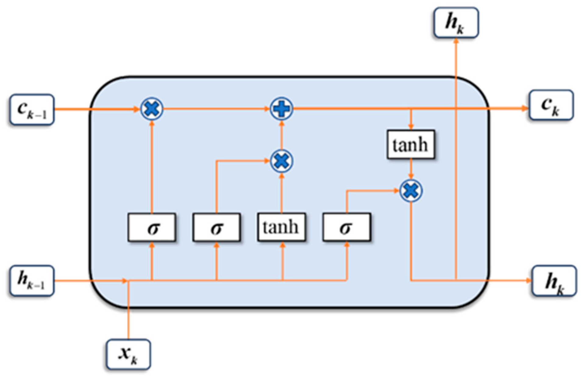
The basic unit structure of LSTM consists of a memory cell, forget gate, input gate, and output gate. These components are designed to control the flow of information and manage memory. The structure is illustrated in Figure 4. The information in LSTM is primarily transmitted through two hidden states within the unit structure: the long-term state c k and the short-term state h k . In the preceding unit structure, the long-term state c k 1 , through the forget gate, selects the information to be forgotten. Subsequently, through the input gate, it decides how much new information to input, forming a new long-term state c k . The long-term state c k is then transmitted to the next unit structure, and simultaneously, the output gate determines how much information from the long-term state should be output to the short-term state. The short-term state h k 1 from the preceding memory unit is integrated with the new unit input x k to form a new input vector. This vector enters the long-term state through the input gate. Simultaneously, by combining with the output gate’s decision on which part of the long-term state information to retain, a new short-term state h k is formed.
The LSTM unit cleverly employs gate mechanisms (forget gate, input gate, and output gate), along with sigmoid and tanh activation functions. It precisely controls state updates by weighting input information. The update rules are formulated as follows:
{ f k = σ ( W f [ x k , h k 1 ] + b f ) i k = σ ( W i [ x k , h k 1 ] + b i ) c ^ k = tanh ( W c [ x k , h k 1 ] + b c ) c k = f k c k 1 + i k c ^ k o k = σ ( W o [ x k , h k 1 ] + b o ) h k = o k tanh ( c k )
where f k represents the forget gate; i k represents the input gate; o k represents the output gate; c ^ k represents the input to the long-term state; c k represents the long-term state; c k represents the short-term state; σ represents the non-linear sigmoid function; W f , W i , W c and W o represent the corresponding weight parameters; b f , b i , b c and b o represent the corresponding bias parameters.
To establish a neural network predictive model for the DOC outlet temperature, dynamic sample data are required. To better capture the dynamic variations of DOC under various operating conditions, the World Harmonized Transient Cycle (WHTC) is chosen as the experimental scenario in regeneration mode. Due to the requirement of the DOC system for an inlet temperature of 250 °C or above, the WHTC in its thermal mode is chosen as the experimental scenario. Experimental results are recorded using INCA, with a sampling frequency of 1 s, and each cycle lasts for 1800 s, resulting in a total of 1801 data sets. For the model development, 70% of the data (1261 sets) are selected as training samples, and the remaining 30% (540 sets) are used as test samples. An offline predictive model based on the LSTM neural network is then established.
For the obtained training data, differences in scales among variables may hinder the convergence of the model during training. To improve the convergence speed and prediction accuracy during the model training process, normalization of the data is necessary. Therefore, the following normalization formula is applied to the aforementioned data:
x = x x min x max x min
where x represents the input data; x min is the minimum value of the input data; x max is the maximum value of the input data; x represents the normalized value corresponding to x .
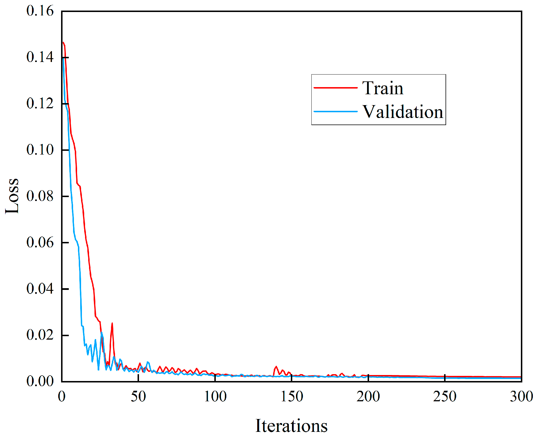
To train the LSTM predictive model, the MatlabR2023a Deep Learning Toolbox was utilized, and the Adam algorithm was employed to accelerate the model training speed, thereby avoiding local minima. The specific training information and parameter settings are detailed in Table 4. Figure 5 illustrates the relationship between the training loss function and validation loss function during the model training iteration process. From the graph, it can be observed that within the limited number of iterations, as the loss function reaches its minimum value, both training and validation losses gradually decrease with increasing iterations. After some oscillations, they eventually converge. This indicates successful model training, with no occurrences of underfitting or overfitting.
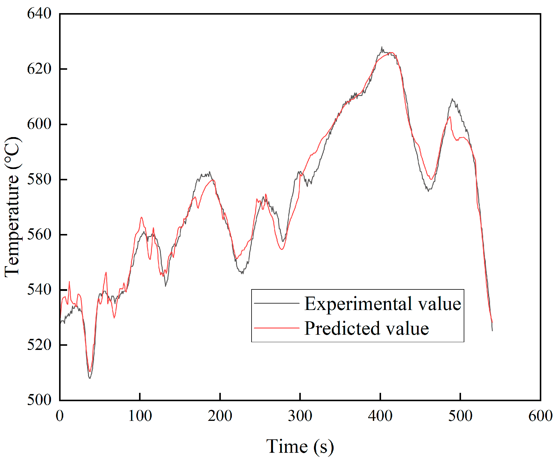
The comparison between the predicted results of the model and the actual values is shown in Figure 6. The predicted results of the model closely align with the actual values, accurately capturing the changing trend of the DOC outlet temperature. To further assess the performance and accuracy of the prediction model, three evaluation metrics, namely Root Mean Squared Error (RMSE), Mean Absolute Error (MAE), and R-squared (R2), are used. Their formulas are as follows:
R M S E = i = 1 n ( y i y i ) y i
M A E = 1 n i = 1 n | y i y i |
R 2 = 1 i = 1 n ( y i y i ) 2 i = 1 n ( y i y ¯ ) 2
where n is the sample quantity; y i is the actual value of the i sample; y i is the predicted value of the i sample; y ¯ is the mean of the actual values.
The evaluation metrics for the LSTM-based DOC outlet temperature prediction model are as follows: RMSE is 3.268, MAE is 4.163, R2 is 96.844%. These metrics indicate that the predictive model performs well, and its accuracy is sufficient to meet the requirements for controller design.

3.2. Reference Trajectory and Feedback Correction

To ensure the smooth operation of the control system, the reference trajectory needs to be designed as a smooth curve, allowing the actual output to transition smoothly toward the setpoint.
y r ( k + i ) = a r i y ( k ) + ( 1 a r i ) y s i = 1 , 2 ,
where a r i is the smoothing factor, and 0 < a r i < 1; y s is the reference setpoint.
Due to errors in the identification model and the presence of external disturbances, there is a certain deviation between the optimization solution in model control and the actual effect. Utilizing feedback correction can, to some extent, reduce the errors introduced by this deviation. Taking the prediction error e ( k ) between the DOC outlet temperature y p ( k ) predicted by the neural network model at time k and the actual output DOC outlet temperature y ( k ) as the prediction error, multiplying it by the feedback correction scaling factor η ́ , and applying it to the next time step to correct the correction value y m ( k + 1 ) . The formula can be expressed as:
e ( k ) = y p ( k ) y ( k )
y m ( k + 1 ) = y p ( k + 1 ) + η ́ e ( k )

3.3. Optimization Solution Based on Gradient Descent Method

Rolling optimization adjusts the optimization control strategy within a finite number of time steps to optimize the value of the performance index function, determining the optimal control input to achieve the system’s optimal performance. The main goal of DOC outlet temperature control is to minimize the difference between the outlet temperature and the target value. Therefore, its performance index function can be defined as:
J ( k ) = i = 1 N p [ y ^ r ( k + i ) y ^ m ( k + i ) ] T λ y [ y ^ r ( k + i ) y ^ m ( k + i ) ] + i = 1 N u [ Δ u ( k + i ) T λ u Δ u ( k + i ) ]
s . t . u min u u max
where y ^ r is the target temperature; N p and N u are prediction time domain and control time domain, respectively ( N p > N u ); λ y and λ u are the weight factors; Δ u is the change of the control law; u min and u max are the minimum and maximum values of the control quantity u, respectively.
The performance index function can be equivalent to a quadratic form:
J ^ ( k ) = 1 2 [ E ^ ( k ) T E ^ ( k ) + ρ ^ Δ u ( k ) T Δ u ( k ) ]
where E ^ ( k ) = [ y ^ r ( k + 1 ) y ^ m ( k + 1 ) , y ^ r ( k + 2 ) y ^ m ( k + 2 ) , , y ^ r ( k + N p ) y ^ m ( k + N p ) ] T represents the error vector; Δ u ( k ) = [ Δ u ( k + 1 ) , Δ u ( k + 2 ) , , Δ u ( k + N p ) ] represents the control increment vector; ρ ^ = d i a g [ ρ 1 , ρ 2 , , ρ N u ] represents the control weight matrix.
In order to obtain the optimal control quantity, the gradient descent method is used to solve the performance index function to obtain the control increment vector:
u ( k + 1 ) = u ( k ) + Δ u ( k ) = u ( k ) - η J ^ ( k ) u ( k )
where η is the adaptive rate of gradient descent method.
Obtain by differentiating Equation (23) with respect to u ( k ) :
J ^ ( k ) u ( k ) = ( E ^ ( k ) u ( k ) ) T E ^ ( k ) + ρ ^ Δ u ( k ) = H ^ ( k ) T E ^ ( k ) + ρ ^ Δ u ( k )
Bring Formula (25) into Formula (24):
u ( k + 1 ) = u ( k ) η H ^ ( k ) T E ^ ( k ) η ρ ^ Δ u ( k )
Δ u ( k ) = η H ^ ( k ) T E ^ ( k ) η ρ ^ + 1
where:
H ^ ( k ) = [ y ^ ( k + 1 ) u ( k ) 0 0 y ^ ( k + 2 ) u ( k ) y ^ ( k + 2 ) u ( k + 1 ) 0 y ^ ( k + N p ) u ( k ) y ^ ( k + N p ) u ( k + 1 ) y ^ ( k + N p ) u ( k + N u 1 ) ] N p × N u
The literature shows that when the control time domain N u is 1, it can not only overcome the difficult problem of large-scale matrix operation, but also obtain satisfactory control effect [32]. Therefore, N u = 1 is set in this paper; Equation (28) can be expressed as:
g ( k ) = H ^ ( k ) = [ y ^ ( k + 1 ) u ( k ) , y ^ ( k + 2 ) u ( k ) , y ^ ( k + N p ) u ( k ) ] T
By inserting Equation (29) into (27), the control rate increment Δ u ( k ) can be expressed as:
Δ u ( k ) = η η ρ ^ + 1 g ( k ) T E ^ ( k )
And when the performance index function is minimum or Δ u ( k ) = 0 , the optimal control quantity u ( k ) is obtained as the controller control quantity.

4. Simulation Experiment and Result Analysis

To validate the predictive control performance of the proposed LSTM-MPC controller in the DOC temperature rise system, combined with the first-order plus time-delay transfer function identified in Section 2 for the DOC temperature rise system, tracking performance and disturbance rejection simulations were conducted in Matlab/Simulink. The LSTM-MPC control strategy was compared and analyzed against PID control.

4.1. Setpoint Tracking Performance Experiment

To validate the setpoint tracking performance of the controllers, the target temperature for the DOC outlet temperature was set to 600 °C. After each controller reached the set target value, the target temperature was reduced by 50 °C at time t = 500 s. The response results of each controller to the setpoint tracking of the target temperature, considering the transfer function of the DOC temperature rise system under different operating conditions, are illustrated in Figure 7.
From Figure 7, Setpoint tracking experiments under three operating conditions (1200 r/min 50 N·m, 1800 r/min 150 N·m and 2400 r/min 250 N·m) show that the LSTM-MPC system has a significant control advantage when the target temperature changes. It can be observed that both LSTM-MPC and PID control can effectively achieve setpoint tracking. At times t = 0 s and t = 500 s, the actual temperature under each controller is maintained for some time at the initial temperature due to the inherent time delay of the controlled system. However, calculations show that, compared with PID, the time for the DOC outlet temperature under LSTM-MPC control to reach the target temperature for the first time was shortened by 21.08, 15.58, and 6.91 s, respectively. The overshoot was reduced by 39.4%, 36.6%, and 17.31%, respectively, and the average time to reach the stable state was reduced by 55.17, 40.51, and 13.02 s. It can be seen from the data that the longer the delay time of LSTM-MPC in the DOC system, the more obvious the improvement of the control effect. This is due to the fact that in systems with time delays, traditional PID controllers may have difficulty quickly adapting to changes because the PID feeds back only based on the current error information. By predicting the future state of the system, LSTM-MPC can deal with the time delay more effectively and adjust the control strategy in advance. Therefore, LSTM-MPC provides faster response, lower overshoot, and comparable steady-state performance in controlling the DOC outlet temperature compared to conventional PID control.

4.2. Disturbance Rejection Performance Simulation Experiment

To validate the disturbance rejection performance of the controllers, the target temperature was set to 600 °C. After the controlled system reached stability, step disturbance signals were introduced at times t = 50 s and t = 450 s. At time t = 50 s, the inlet temperature was decreased by 50 °C, and at time t = 450 s, the inlet temperature was increased by 30 °C. The response curves of each controller to the transfer function of the DOC temperature rise system under different operating conditions are shown in Figure 8.
From Figure 8, it can be observed that after introducing disturbances at times t = 50 s and t = 450 s, both LSTM-PID and PID control maintain the outlet temperature at the target value for some time (due to the inherent time delay of the controlled system) before experiencing a sharp decrease (or increase). In PID control, the DOC outlet temperature continues to exhibit a time lag after the sharp decrease (or increase) because PID control primarily relies on feedback regulation, and adjustments to the control strategy are made only after the feedback of the changed DOC outlet temperature. However, the LSTM-MPC controller, leveraging predictive modeling to anticipate the future behavior of the system, adjusts the control strategy in real time upon introducing disturbances. As a result, the DOC outlet temperature responds promptly after the system’s time lag. Additionally, LSTM-MPC control has a smaller overshoot than PID control, which is reduced by 35.65%, 34.66% and 28.89%, respectively, and the average time to reach the stable state is shortened by 93.26, 58.13 and 28.72 s, respectively. From this, it is evident that LSTM-MPC control demonstrates robustness in dealing with time-delay systems, effectively addressing uncertainties and changes in time delay to some extent. Furthermore, the LSTM-MPC controller proves effective in suppressing the impact of disturbances during control, resulting in significantly enhanced disturbance rejection compared to conventional PID controllers.

5. Conclusions

In this paper, we introduce the LSTM prediction model and gradient descent method, proposing a nonlinear predictive control method for DOC outlet temperature named LSTM-MPC. By offline training the LSTM neural network, real-time prediction of the DOC outlet temperature for diesel engines is achieved, providing a high-precision predictive model for MPC.
(1)
LSTM-MPC employs the gradient descent algorithm to solve nonlinear optimization problems, aiming to reduce the computational time for optimization solutions and achieve optimal control rates for fuel injection heating.
(2)
LSTM-MPC is compared with PID control in terms of tracking performance and disturbance rejection capability through simulation. In the set point tracking experiment, the average time to first reach the set temperature is reduced by 14.61 s, the average overshoot is reduced by 35.9%, and the average time to reach the steady state is reduced by 36.23 s. In the experiment of anti-interference performance, the average overshoot is reduced by 33.89%, and the average time to reach the stable state is reduced by 60.04 s. The results indicate that this control strategy exhibits fast response, good tracking performance, and strong disturbance rejection capabilities. Additionally, the strategy can effectively reduce the influence of time delay on the system, and its theoretical control effect in the DOC outlet temperature control process is proved by simulation experiments. We will further verify its control effect in engineering applications in future work.

Author Contributions

Conceptualization, X.Y., G.W. and Y.W.; methodology, X.Y.; software, X.Y.; validation, X.Y., G.W. and Q.S.; formal analysis, X.Y.; investigation, X.Y., Y.W., Q.S. and B.Z.; resources, S.H.; data curation, S.H.; writing—original draft preparation, X.Y.; writing—review and editing, X.Y., G.W. and Y.W.; visualization, Q.S. and B.Z. All authors have read and agreed to the published version of the manuscript.

Funding

This research was funded by the Innovation Guidance and Technology-based Enterprise Cultivation Program of Science and Technology Department of Yunnan Province, grant number (202104BN050007), funder: G.W.; and the Major Science and Technology Special Program of Science and Technology Department of Yunnan Province, grant number (202102AC080004), funder. G.W.

Data Availability Statement

Data is contained within the article.

Conflicts of Interest

Author Shuchao He is employed by the company Kunming Yunnei Power Co., Ltd.; The remaining authors declare that the research was conducted in the absence of any commercial or financial relationships that could be construed as a potential conflict of interest.

References

  1. Johnson, T. Vehicular emissions in review. SAE Int. J. Engines 2016, 9, 1258–1275. [Google Scholar] [CrossRef]
  2. Wu, Y.; Zhang, S.; Hao, J.; Liu, H.; Wu, X.; Hu, J.; Walsh, M.P.; Wallington, T.J.; Max Zhang, K.; Stevanovic, S. On-road vehicle emissions and their control in China: A review and outlook. Sci. Total Environ. 2017, 574, 332–349. [Google Scholar] [CrossRef] [PubMed]
  3. Wang, J.; Wu, Q.; Liu, J.; Yang, H.; Yin, M.; Chen, S.; Guo, P.; Ren, J.; Luo, X.; Linghu, W.; et al. Vehicle emission and atmospheric pollution in China: Problems, progress, and prospects. PeerJ 2019, 7, e6932. [Google Scholar] [CrossRef] [PubMed]
  4. Ayodhya, A.S.; Narayanappa, K.G. An overview of after-treatment systems for diesel engines. Environ. Sci. Pollut. Res. 2018, 25, 35034–35047. [Google Scholar] [CrossRef] [PubMed]
  5. Reşitoğlu, İ.A.; Altinişik, K.; Keskin, A. The pollutant emissions from diesel-engine vehicles and exhaust aftertreatment systems. Clean Technol. Environ. Policy 2015, 17, 15–27. [Google Scholar] [CrossRef]
  6. Kurien, C. Review on post-treatment emission control technique by application of diesel oxidation catalysis and diesel particulate filtration. J. Therm. Eng. 2019, 5, 108–118. [Google Scholar] [CrossRef]
  7. Lao, C.T.; Akroyd, J.; Eaves, N.; Smith, A.; Morgan, N.; Nurkowski, D.; Bhave, A.; Kraft, M. Investigation of the impact of the configuration of exhaust after-treatment system for diesel engines. Appl. Energy 2020, 267, 114844. [Google Scholar] [CrossRef]
  8. Zhang, Z.; Dong, R.; Lan, G.; Yuan, T.; Tan, D. Diesel particulate filter regeneration mechanism of modern automobile engines and methods of reducing PM emissions: A review. Environ. Sci. Pollut. Res. 2023, 30, 39338–39376. [Google Scholar] [CrossRef]
  9. Shi, Y.; Lu, Y.; Cai, Y.; He, Y.; Zhou, Y.; Fang, J. Evolution of particulate matter deposited in the DPF channel during low-temperature regeneration by non-thermal plasma. Fuel 2022, 318, 123552. [Google Scholar] [CrossRef]
  10. Rothe, D.; Knauer, M.; Emmerling, G.; Deyerling, D.; Niessner, R. Emissions during active regeneration of a diesel particulate filter on a heavy duty diesel engine: Stationary tests. J. Aerosol Sci. 2015, 90, 14–25. [Google Scholar] [CrossRef]
  11. Liu, G.; Liu, W.; He, Y.; Gong, J.; Li, Q. Research on influence of exhaust characteristics and control strategy to DOC-assisted active regeneration of DPF. Processes 2021, 9, 1403. [Google Scholar] [CrossRef]
  12. Bai, S.; Chen, G.; Sun, Q.; Wang, G.; Li, G.X. Influence of active control strategies on exhaust thermal management for diesel particular filter active regeneration. Appl. Therm. Eng. 2017, 119, 297–303. [Google Scholar] [CrossRef]
  13. Lapuerta, M.; Rodríguez-Fernández, J.; Oliva, F. Effect of soot accumulation in a diesel particle filter on the combustion process and gaseous emissions. Energy 2012, 47, 543–552. [Google Scholar] [CrossRef]
  14. Wan, M.; Xiao, B.; Bi, Y.; Tang, C.; Shen, L.; Lei, J. Experimental study on temperature characteristics of DPF substrate for active regeneration in plateau environment. Trans. Chin. Soc. Agric. Eng. 2020, 36, 121–128+328. [Google Scholar]
  15. Liu, H.; Zhang, K.; Yao, G.; Zhang, W.; Zi, X. A Research on DOC Assisted DPF Regeneration Technology with In-cylinder Fuel Post-Injection and Exhaust-pipe Fuel Injection. Automot. Eng. 2015, 37, 391–395. [Google Scholar]
  16. Lepreux, O.; Creff, Y.; Petit, N. Model-based control design of a diesel oxidation catalyst. IFAC Proc. Vol. 2009, 42, 279–284. [Google Scholar] [CrossRef]
  17. Su, C.; Brault, J.; Munnannur, A.; Liu, Z.G.; Milloy, S.; Harinath, A.; Dunnuck, D.; Federle, K. Model-based approaches in developing an advanced aftertreatment system: An overview. SAE Int. J. Adv. Curr. Pract. Mobil. 2019, 1, 201–214. [Google Scholar] [CrossRef]
  18. Guardiola, C.; Pla, B.; Piqueras, P.; Mora, J.; Lefebvre, D. Model-based passive and active diagnostics strategies for diesel oxidation catalysts. Appl. Therm. Eng. 2017, 110, 962–971. [Google Scholar] [CrossRef]
  19. Regaya, C.B.; Farhani, F.; Zaafouri, A. Adaptive proportional-integral fuzzy logic controller of electric motor drive. Eng. Rev. 2021, 41, 26–40. [Google Scholar] [CrossRef]
  20. Regaya, C.B.; Zaafouri, A.; Chaari, A. A new sliding mode speed observer of electric motor drive based on fuzzy-logic. Acta Polytech. Hung. 2014, 11, 219–232. [Google Scholar]
  21. Regaya, C.B.; Farhani, F.; Zaafouri, A.; Chaari, A. High-performance control of IM using MRAS-fuzzy logic observer. Int. J. Tomogr. Simul. 2017, 30, 40–52. [Google Scholar]
  22. Regaya, C.B.; Farhani, F.; Hamdi, H.I.C.H.E.M.; Zaafouri, A.; Chaari, A. Robust ANFIS vector control of induction motor drive for high-performance speed control supplied by a photovoltaic generator. WSEAS Trans. Syst. Control 2020, 15, 356–365. [Google Scholar] [CrossRef]
  23. Kim, Y.W.; Van Nieuwstadt, M.; Stewart, G.; Pekar, J. Model predictive control of DOC temperature during DPF regeneration. SAE Tech. Pap. 2014, 1, 1165. [Google Scholar]
  24. Huang, T.; Hu, G.; Meng, Z.; Zeng, D. Exhaust temperature control for safe and efficient thermal regeneration of diesel particulate filter. Appl. Therm. Eng. 2021, 189, 116747. [Google Scholar] [CrossRef]
  25. Caliskan, H.; Mori, K. Environmental, enviroeconomic and enhanced thermodynamic analyses of a diesel engine with diesel oxidation catalyst (DOC) and diesel particulate filter (DPF) after treatment systems. Energy 2017, 128, 128–144. [Google Scholar] [CrossRef]
  26. Lepreux, O.; Creff, Y.; Petit, N. Model-based temperature control of a diesel oxidation catalyst. J. Process Control 2012, 22, 41–50. [Google Scholar] [CrossRef]
  27. Wu, F.; Zhang, B.; Yao, D.; Yang, Y. Modeling and Order Reduction for the Thermodynamics of a Diesel Oxidation Catalyst with Hydrocarbon Dosing. Catalysts 2019, 9, 369. [Google Scholar] [CrossRef]
  28. Liu, H.; Gao, Y.; Ma, B.; Li, F.; Yin, Y.; Xie, T. Investigation on Temperature Control of Diesel Oxidation Catalyst Outlet. Trans. Chin. Soc. Agric. Mach. 2018, 49, 387–392. [Google Scholar]
  29. Huang, T.; Hu, G.; Yan, Y.; Zeng, D.; Meng, Z. Combined feedforward and error-based active disturbance rejection control for diesel particulate filter thermal regeneration. ISA Trans. 2023, 134, 28–41. [Google Scholar] [CrossRef]
  30. Mayne, D.Q. Model predictive control: Recent developments and future promise. Automatica 2014, 50, 2967–2986. [Google Scholar] [CrossRef]
  31. Chen, P.; Wang, J. Nonlinear model predictive control of integrated diesel engine and selective catalytic reduction system for simultaneous fuel economy improvement and emissions reduction. J. Dyn. Syst. Meas. Control 2015, 137, 081008. [Google Scholar] [CrossRef]
  32. Lu, C.H. Wavelet fuzzy neural networks for identification and predictive control of dynamic systems. IEEE Trans. Ind. Electron. 2011, 58, 3046–3058. [Google Scholar] [CrossRef]
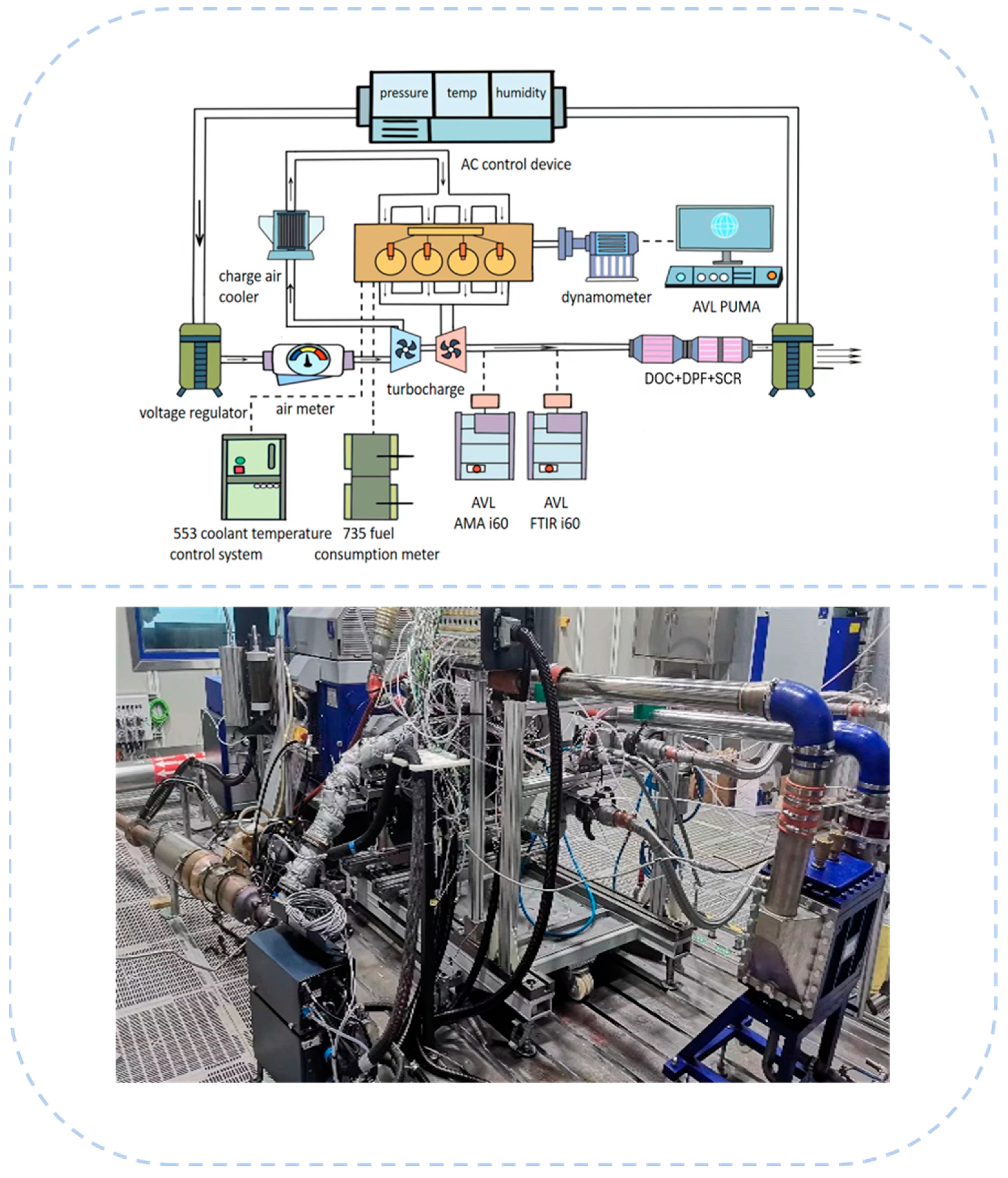
Figure 1. Physical photograph (below) and schematic layout (above) of the engine test bench.
Processes 12 00225 g001
Figure 2. Experimental and simulated value comparison under different operating conditions. (a) 1200 r/min 50 N·m, u = 0.3 mg. (b) 1800 r/min 150 N·m, u = 0.36 mg. (c) 2400 r/min 250 N·m, u = 0.24 mg.
Processes 12 00225 g002
Figure 3. Basic structure diagram of the control algorithm.
Processes 12 00225 g003
Figure 4. Basic unit structure of LSTM.
Processes 12 00225 g004
Figure 5. Change in loss values of LSTM predictive model with iteration count.
Processes 12 00225 g005
Figure 6. Comparison of predictions from different predictive models.
Processes 12 00225 g006
Figure 7. Tracking setpoint temperature responses under various operating conditions. (a) 1200 r/min 50 N·m. (b) 1800 r/min 150 N·m. (c) 2400 r/min 250 N·m.
Processes 12 00225 g007
Figure 8. Response curve of DOC outlet temperature with added disturbance. (a) 1200 r/min 50 N·m. (b) 1800 r/min 150 N·m. (c) 2400 r/min 250 N·m.
Processes 12 00225 g008
Table 1. Basic parameters of the diesel engine.
Parameter TypeNumerical Value
Diesel engine type4-cylinder inline, 4 valves, turbocharged
Bore × Stroke (mm × mm)92 × 94
Displaced volume (L)2.5
Compression ratio17.5:1
Maximum torque (N·m)400
Rated speed (r/min)3000
Power rating (kW)120
Table 2. Specifications of the DOC.
Parameter TypeNumerical Value
DOC SubstrateCordierite
Length (mm)152.4
Diameter (mm)122
Cell density (cpsi)400
Table 3. Identification parameters and fitting accuracy of first-order time delay transfer function model.
Speed (r/min)Torque (N·m)kTcτAccuracy (%)
120050944.9124.22341.33192.52
1800150394.7811.67718.46293.15
2400250384.87.35139.326593.33
Table 4. Structural parameters of the LSTM-based predictive model for DOC outlet temperature.
NameNumerical Value
OptimizerAdam
Activation functionSigmoid, tanh
Maximum iterations300
Gradient decay rate0.99
Learning rate decline cycle175
Initial learning rate0.05
Learning rate decline coefficient0.001
Disclaimer/Publisher’s Note: The statements, opinions and data contained in all publications are solely those of the individual author(s) and contributor(s) and not of MDPI and/or the editor(s). MDPI and/or the editor(s) disclaim responsibility for any injury to people or property resulting from any ideas, methods, instructions or products referred to in the content.