
Resolved Simulation of the Clarification and Dewatering in Decanter Centrifuges
by
 ,
,
Helene Katharina Baust
1,* ,
,
Simon Hammerich
2,
Hartmut König
2,
Hermann Nirschl
1 and
Marco Gleiß
1 1
Institute of Mechanical Process Engineering and Mechanics, Karlsruhe Institute of Technology, Straße am Forum 8, 76131 Karlsruhe, Germany
2
BASF SE, Carl-Bosch-Strasse 38, 67056 Ludwigshafen am Rhein, Germany
*
Author to whom correspondence should be addressed.
Processes 2024, 12(1), 9; https://doi.org/10.3390/pr12010009
Submission received: 18 October 2023
/
Revised: 4 December 2023
/
Accepted: 15 December 2023
/
Published: 19 December 2023
(This article belongs to the Special Issue 10th Anniversary of Processes: Design of the Chemical Industry of the Future)
Abstract
:Solid–liquid separation is a fundamental operation in process engineering and thus an important part of many process chains in the preparation of slurries in the chemical industry and other parts of the industrial environment. For the separation of micron-sized particles which, due to their size, do not settle or settle very slowly in the earth’s gravity field, centrifuges are often used. The preferred choice are often decanter centrifuges because they work continuously and stabilize the process against product fluctuations due to their adjustment possibilities. The design of the apparatus is complex: The main components of the apparatus are the cylindrical-conical bowl, which rotates at a high speed, and a screw located inside the bowl, which rotates in the same direction at a low differential speed to transport the separated solids out of the apparatus. Geometrical properties of the apparatus, as well as the adjustable operating parameters, such as rotational speed or differential speed, have a significant influence on the separation. In practice, analytical models and the experience of the manufacturers form the basis for the design. Characteristics of the disperse phase, interactions with the liquid, as well as the influence of the flow on the separation, are not taken into account. As a consequence, the transfer to industrial scale always requires a large number of pilot-scale experiments, which are time-consuming and expensive. Due to the increasing computational power, computational fluid dynamics (CFD) provides one possibility to minimize the experimental effort in centrifuge design. In this work, the open-source software OpenFOAM is used to simulate the multi-phase flow in a laboratory decanter centrifuge. For validation, experiments were carried out on a laboratory scale and the main operating parameters, such as speed, differential speed, and volume flow rate, were varied. The simulation results show a good agreement with the experimental data. Furthermore, the numerical investigations show the influence of the flow on the separation of the particles. To evaluate the transportability of a material, the transport efficiency was introduced as a dimensionless parameter. In addition, the simulation allows the consideration of the individual velocity components, making it possible to generate an impression of the complex three-dimensional flow in the apparatus for the first time.
1. Introduction
Decanter centrifuges are continuously operating centrifuges that are frequently used for solid–liquid separation. For example, they find use on an industrial scale in the chemical or food industry, but also in wastewater treatment and mining. Due to their complex design and the high speeds at which decanter centrifuges rotate, the experimental investigation of the separation processes in the apparatus is difficult. This complicates the design and dimensioning of the centrifuge as well as the determination of ideal operating conditions, which entails high costs [1].
At this point, numerical simulations help to increase the understanding of the process and optimize the design of the centrifuges and the separation process. On the one hand, dynamic real-time models exist, which cannot resolve the process directly, but provide a fast estimation of the process behavior with low computational effort by means of additional assumptions. For the compensation of the necessary model reduction, the flow and material behavior are modeled by suitable material and machine functions. On the other hand, there are resolved flow simulations that give more detailed insights into the physical behavior of centrifuges. In computational fluid dynamics (CFD), the flow pattern of the continuous phase is described by the solution of the Navier–Stokes equations and is thus resolved temporally and spatially. There are different methods for modeling the disperse phase: In Eulerian–Eulerian two-phase flows, the dispersed phase is also treated as a fluid, and additional conservation equations are solved. Supplemental source terms allow the momentum exchange between the two phases to be taken into account. In the Eulerian–Lagrange method, the dispersed phase is modeled using discrete moving particles on a co-moving coordinate system. The motion of the particles results from the forces acting on the particles due to, for example, fluid flow and particle–particle interactions. But again, the momentum exchange between the phases requires additional source terms. The disadvantage of resolved simulations is the high computational time, which is further increased by the additional source terms for the consideration of the interaction between the continuous and dispersed phases.
The literature contains a number of real-time models: Stickland et al. [2] developed a model for the simulation of batch centrifuges, tubular centrifuges and the cylindrical part of decanter centrifuges. It is based on a one-dimensional numerical model for discontinuous bucket centrifuges. Thereby, three different domains of behavior exist: clarified fluid, sedimentation, and sediment compression. To represent the unsteady behavior, the conservation equations of momentum and mass are described with the Runge–Kutta method and linked to the flux density function based on the work of Kynch [3]. The consideration of the material behavior enables a realistic simulation of the process. Building on the idea of flow sheet simulation [4,5], numerical models require a model reduction to simulate unit operations in real time. This makes it possible to model individual apparatuses as well as entire process chains [6]. Applied to a solid bowl centrifuge, it is possible to calculate the separation efficiency and the sediment build-up. Thereby, this model also takes into account the geometry of the apparatus and machine functions. Gleiß et al. [7] and Menesklou [8] have developed such a model for decanter centrifuges. Empirical equations and model assumptions allow the characterization of the separation process. To describe the stratified flow patterns, a parabolic velocity profile was assumed. To describe the transport of the sediment or its efficiency, the authors introduce an additional factor that ranges from 0 to 1, where 0 stands for no transport and 1 for complete transport. To take into account the influence of local flow effects on the separation behavior, Menesklou [8] extended the dynamic model with a neural network. The literature presents various hypotheses regarding the flow in decanter centrifuges: some assume a parabolic flow profile [7], others plug flow [9]. Furthermore, experiments have shown that backflow may occur immediately above the sediment [10,11]. Bai et al. [12,13] have also developed a dynamic model for decanter centrifuges and propose a new flow model that combines the parabolic flow profile and the backflow above the sediment according to a model proposed by Amirante and Catalano [14]. The calculation of the cut size of the particle system is performed by different drag models as a function of the Reynolds number. The models already presented [7,8,12,13,14] solely model the sedimentation and sediment formation. Furthermore, it is unclear whether the material is transportable or not. Bell et al. [15] have developed a mathematical model that describes sediment transport in decanter centrifuges, taking into account the power, torque, and necessary axial force of the screw to ensure transportability. The model was validated for granular products with data from Reif and Stahl [16].
The flow of the continuous phase in the apparatus has a direct effect on the movement of the particulate phase; thus, the flow conditions significantly influence the separation. To better understand the interplay between flow and separation behavior, resolved simulations are essential: Romaní Fernández and Nirschl [17] proposed a coupled CFD–DEM method for the simulation of a solid bowl centrifuge. CFD provides the simulation of the flow of air and water, while DEM serves to model the movement of the particles. However, the computational effort rises with increasing particle number. The simulation of finely dispersed particle systems (<20 ) and their consolidation behavior would obviously require a high computational effort. For this reason, Hammerich et al. [18] developed a multi-phase simulation model for tubular centrifuges. The multi-phase system was treated as a mixed phase, with additional transport equations solved for the solid volume fraction. The model takes into account the consolidation and rheological behavior of the sediment. The sediment build-up over time has a strong influence on the flow conditions, which is in agreement with experimental data. Due to solver-internal algorithms and equations, the model is not applicable to complex geometries, such as the decanter centrifuge. Zhu et al. [19] studied the solids distribution in a decanter centrifuge with a steady-state simulation. The simulation was performed with the software Fluent and the continuous and dispersed phases were calculated with the Eulerian–Eulerian method. The simulation results were compared with experiments. However, the simulated solids fraction was higher than expected (>85 ). Kang et al. [20] also modeled the multi-phase system with the Eulerian two-phase model. A multi-parameter optimization indicates possibilities for improving the separation performance in decanter centrifuges. For this purpose, geometrical properties, such as window size and the presence of a gap, were varied. Garrido et al. [21] have shown that the sedimentation–consolidation process in centrifuges can be described by a single partial differential equation using solely one scalar, the solids volume fraction. Therefore, it is necessary to define initial and boundary conditions. Batch centrifuge tests [22,23] are used for validation, whereby the model achieved a good agreement. Based on these results, Baust et al. [24] have coupled the partial differential equation with the conservation equations for the flow in CFD. Material functions provide the basis for modeling to consider the interactions between the continuous and dispersed phases. In contrast to the solver of Hammerich et al. [18], the partial differential equation for the volume fraction of the solids allows the simulation of complex geometries. Moreover, additional equations, as in the conventional Euler–Euler or Euler–Lagrange models, are not necessary, which is why the computation time is comparatively moderate.
The specific objective of this study was to apply the solver developed by Baust et al. [24] to a decanter centrifuge. The variation of the operating parameters served to verify the model in order to test whether it reproduces different characteristics of clarification and dewatering in decanter centrifuges. Experiments on a laboratory centrifuge were used for validation. The resolved simulation also provided insight into the flow processes in the apparatus. By studying the different velocity components, it was possible to identify and describe different flow phenomena in the apparatus. Furthermore, this study proposes to derive a transport efficiency from CFD data.
2. Materials and Methods
This section provides an overview of the numerical and experimental methods that form the basis for the numerical investigation of the separation behavior and the flow behavior in decanter centrifuges. The solids transport was calculated by means of an additional transport equation for the solids volume fraction. Required material functions were derived from laboratory experiments. The experimental and numerical investigations were carried out with a decanter centrifuge on a laboratory scale.
2.1. Numerical Setup
CFD is a mathematical method for calculating the pressure and velocity of single-phase or multi-phase flows. It is based on continuum mechanics and uses the finite volume method for the discretization of differential equations. The mathematical description comprises the conservation of mass, momentum, and energy for the flowing fluid. For the numerical study of the flow in decanter centrifuges, the solid particles and the liquid are considered a single mixed phase, and the dispersed phase was modeled by an additional partial differential equation [24]. Thereby, the following assumptions applied:
- A1
- The gas phase was neglected.
- A2
- All particles had the same size, shape, and density.
- A3
- Both the particles and the fluid were incompressible.
- A4
- There was no mass transfer between the components.
- A5
- The interactions between the disperse and continuous phases were taken into account by an additional transport equation for the solid volume fraction. Thereby, the settling velocity as well as the consolidation and viscosity depended solely on the solids volume fraction.
- A6
- Wall effects were not considered.
In this work, solely the conservation equations for the mass and the momentum were relevant. The mass
and the momentum balance
for an incompressible and Newtonian fluid can be derived from a differential balance around a control volume and depend on the velocity vector . Further, describes the partial derivative with respect to time t, p is the pressure, is the density and the kinematic viscosity of the mixture. An additional transport equation of the solids volume fraction provided the modeling of the dispersed phase.
The equation was proposed by Garrido et al. [21]. The solids volume fraction is defined as the ratio of the particle volume to the total volume .
The individual terms in Equation (3) describe, from left to right, the accumulation of the solids volume fraction, the convective change due to both the flow and the acceleration (sedimentation), and the consolidation of the sediment. Here, r stands for the radius, for the angular velocity, g for the acceleration due to gravity, and , as well as , for the density of the particles and the liquid phase. The unit vector is parallel to the axis of rotation. The other unit vector is orthogonal to and acts in the direction of the acceleration force. To stabilize the transport equation, Garrido’s [21] Equation (3) was extended by the factor , which depends on a critical solids volume fraction, the gel point . The gel point characterizes the transition between slurry and sediment. If , the mixture exists as a slurry, and . If the mixture is present as sediment and . At the transition between slurry and sediment, takes values between 0 and 1, and ensures that there is no abrupt change in the flow properties. The two remaining functions and represent the material functions for the sedimentation behavior and the compressive behavior of the sediment and depend solely on the solids volume fraction.
The dispersed phase does not directly affect the conservation equations; instead, model equations describe the flow behavior of the slurry and sediment by means of the kinematic viscosity of the mixed phase. As a result, additional source terms for the description of the momentum exchange between the continuous and dispersed phases are omitted, which reduces the computing time. To describe the rheological behavior of both the slurry and sediment, the kinematic viscosity consists of two summands that may or may not be considered, depending on the factor .
According to Hammerich et al. [18], the approach of Quemada [25] was used to model the viscosity of the slurry. The sediment flow behavior was described by a Herschel-Bulkley fluid. The variables and represent the dynamic viscosity and the density of the pure liquid, stands for the maximum packing density, is the yield locus of the sediment, K is the consistency, is the flow index, and symbolized the strain rate.
The implementation of this method took place in the open-source software OpenFOAM (v1912, OpenCFD Ltd., Bracknell, UK) based on the solver pimpleFoam. For the discretization of time-dependent partial differential equations, the Courant number
indicates the maximum distance the considered quantity may move per time step. For example, explicit Euler methods are stable for [26,27]. In Equation (6), describes the spatial step increment and the time step increment. In numerical flow simulations, the Courant number ensures that the computational case runs stably. By summing the settling velocity of the particles and the flow velocity of the mixing phase, the particles may reach higher velocity gradients than numerically desired. To avoid instabilities, the function object CourantNo was, therefore, extended by the settling velocity of the particles in this work. A more detailed description of the solver is given by Baust et al. [24].
2.2. Experimental Determined Material Functions
The flux density function is defined as the product of the solids volume fraction, the settling velocity of a single particle (Stokes’ settling velocity), and the hindrance settling factor , which describes the deviation of the actual settling velocity as a function of the solids volume fraction.
In highly diluted slurries, the particles settle according to their size. According to the approach of Stokes [28], the settling velocity of spherical particles is proportional to the square of the particle radius and depends on the density difference between the dispersed and continuous phases, the viscosity of the continuous phase, and the acceleration acting on the particle.
An increased number of particles reduces the distance between the particles and influences the flow area of the particles. Consequently, the settling velocity depends on the solids volume fraction. By measuring the settling velocity of slurries with different solids volume fractions, and relating them to Stokes’ settling velocity , the hindrance settling function may be determined. A commonly used approach to describe the settling hindrance of a monodisperse particle system is the approach of Richardson and Zaki [29].
The exponent is an empirical parameter that assumes the value for Reynolds numbers . A correction to the equation has been proposed by Michaels and Bolger [30] by expanding the equation with the maximum solids volume fraction since the disperse phase fraction is always less than 1.
The sedimentation of the particles leads to an accumulation of particles and finally to the formation of the liquid-saturated sediment on the inner wall of the bowl. The characteristics of the formed sediment, which include its compressibility, strongly depend on particle–particle interactions and on the properties of the disperse phase (e.g., size and shape). For the characterization of sediment structure, the literature [31,32,33,34] provides a large number of models that describe the solids volume fraction as a function of the compressive resistance. Green et al. [33] used a power law to describe the compression behavior.
Here, is the compressive resistance. The parameters and are material specific and derivable from experiments. A detailed description for the experimental determination of the material functions is given by Zhai et al. [35].
Kaolin dispersed in water was used to validate the simulation method. Table 1 lists the corresponding material properties. The density of kaolin is 2600 , that of water 1000 . As the applied solver does not yet take into account polydisperse particle systems, the average particle size was used for the simulation. Kaolin has a mean particle size of 3 and a plate-like shape. This paper emphasizes the functionality of the solver. Since the solver calculates solely monodisperse particle systems so far, the focus is still on the sediment. For this reason, the sedimentation has been calculated in a simplified way with the parameters and for the hindered settling function. The gel point is for the considered slurry. To describe the rheological behavior of the sediment, 1 was assumed for the the yield point, for the consistency, and for the rheological exponent.
Figure 1 shows the consolidation function of the kaolin studied. The empirical parameters have the values Pa and . Kaolin compresses mainly below a compression resistance . A higher compression resistance barely leads to an increase in the volume fraction of the disperse phase. At , a nearly steady state is reached.
2.3. Experimental Setup
To validate the simulation method, experimental investigations on a laboratory-scale decanter centrifuge were compared with the corresponding simulations. Figure 2 shows the experimental setup. A pump conveys the slurry from a stirred tank to the decanter centrifuge MD-80 decanter centrifuge, Lemitec GmbH (Berlin, Germany). The pump allows adjustments to the volumetric flow rate. Immediately before the separator, a three-way valve allows samples to be taken from the feed to measure the solids mass fraction. The decanter centrifuge operates on the counterflow principle and enables the speed of the bowl and differential speed of the screw to be varied. In addition, the weir height is variable, but was kept constant for the present work.
During the measurement process, all process parameters were first set, and afterward, one of the operating parameters, for example, the rotational speed, was varied. After each operating point, the centrifuge was rinsed with water to remove any sediment remaining in the apparatus. This ensures that previous experiments do not influence the current series of measurements. For the characterization of the separation process, the samples were taken after the centrifuge had reached a stationary state. Thereby, sediment and centrate samples were analyzed, whereas the focus of the present publication was on the sediment. The solids mass fraction of the individual samples was determined gravimetrically and then converted into the solids volume fraction .
Here, w stands for the mass fraction of the solids (p) or the liquid (l).
During the validation experiments and the simulation, the volume flow rate, the rotational speed, and the differential speed were varied. For the evaluation, the volume flow rate was expressed by the Reynolds number Re.
The Reynolds number is defined as the ratio between inertial and viscous forces and depends on the flow velocity u, the kinematic viscosity , and the hydraulic diameter . The flow along the helical structure of the screw can be assumed to be a channel flow. The hydraulic diameter depends on the channel width and its height. The rotational frequency was converted to the centrifugal number C.
This dimensionless number describes the acceleration induced by the rotational speed as a multiple of the acceleration due to gravity .
2.4. Geometry and Mesh Generation
For the simulation, a mesh was created according to the geometric dimensions of the laboratory centrifuge. The decanter centrifuge consists of a bowl diameter of 80 and a cone angle of 7°. Related to the radius of the inner wall of the bowl, the centrifuge achieves a maximum centrifugal acceleration of g. Various weir disks enable different pond depths to be set. In this work, a constant pond depth of 10 was used. The wall thickness of the flights was assumed to be 2 . The gap between the tip of the screw and the bowl was not resolved. Figure 3 shows the geometry of the centrifuge. It also shows the division into 13 segments for the evaluation. Moreover, all relevant dimensions are depicted, whose values are listed in Table 2. In total, the centrifuge has a length of 315 , where the cylindrical part is 172 long and the conical part is 143 long.
The geometry was created using the ANSYS DesignModeler (Ansys 2020 R1, Ansys, Inc., Canonsburg, PA, USA). To obtain a structured mesh consisting of preferably uniform hexahedrons, the mesh had to be cut several times and divided into different segments. Here, the start and end of the flights, the inlets, and the transition between the cylindrical and conical parts of the apparatus posed particular challenges. The gap between the tip of the screw and the bowl was not resolved. Finally, the geometry was divided into 157 segments. The mesh generation tool of ANSYS was used to create the mesh itself. Figure 4 presents the geometry generated with the DesignModeler and, as an example, the mesh of two segments at about ten times the magnification of the apparatus shown. The geometry had to be cut at the transition between the cylindrical and conical part to avoid unstructured cells as much as possible. This resulted in a tapered segment at the transition of the cylindrical and conical parts. Additional cuts in the axial direction (here, along the z-axis) ensured that the mesh in the individual screw segments consisted of structured hexahedrons. On the ends of the flights, as well as at the transition between the cylindrical and conical part, the cells are more irregular, which is also where the worst cells are found compared to the rest of the mesh. In the sections immediately before these abrupt end points of the flights, the mesh cells become steadily smaller due to the already increasing taper. Additional cuts were also necessary at the inlets.
To ensure that the resolution of the mesh was sufficiently accurate, the cell size of the mesh was successively reduced and the results of the simulations were compared with each other. For this purpose, , and were specified as the desired element size, resulting in meshes with 600 000, 1300 000 and 2400 000 cell elements. In addition, the mesh quality properties were checked. None of the investigated meshes had a maximum skewness of more than , and the orthogonality never fell below a value of . For the mesh independence study, the velocity distribution and the sediment structure in the screw channel were used as criteria. Figure 5 shows the axial component of the flow velocity (a) and the solids volume fraction (b) as a function of the radial position r in the screw channel for the fourth segment. To save calculation time, the solids volume fraction in the apparatus was pre-patched, which resulted in a faster sediment formation. The differential movement of the screw leads to the transport of the sediment toward the cone. Consequently, the axial velocity assumes a positive value for the sediment part. In contrast, the slurry flows over the sediment in the opposite direction of the weir. Consequently, the axial velocity component is negative. Since the screw channel was completely filled with slurry in this work and the velocity at the screw body is zero and corresponds to its rotational movement, the axial velocity at the screw body is again positive. Overall, the mesh independence study shows that the mesh with an element size of deviates significantly from the simulation results of the finer meshes. The significant difference probably results directly from the larger cells and thus from a different sediment distribution. Looking at the surface integrals, the velocity profile of the coarsest grid deviates by 21% and the profile of the solids volume fraction deviates by 34% from the finest mesh. In contrast, the profiles for the axial velocity component and the solids volume fraction are well represented by the mesh with element size . The deviations are merely 2% for the velocity profile and 3% for the solids volume fraction.
In addition to simulation accuracy, computing time also plays an important role in the selection of the mesh. Thereby, the element size or the number of elements have a decisive influence on the calculation time. The finest mesh required 166 to simulate 1 , while the simulation with the coarsest mesh solely lasted 26 . This means that the simulation of one minute takes longer than 1 day even for the coarsest mesh and 1 week for the finest mesh. The mesh with an element size of offers a compromise. Both the profile of the velocity component and of the solids volume fraction coincide with that of the finest mesh, and the simulation of 60 requires 2.5 days. For these reasons, the decision fell on the mesh with an element size of . Another test case, which was set up to check the transportability in the cone, is based on these results and consists of 700 000 cells.
The flow in the decanter centrifuge was assumed to be the rotation of a rigid body. The dynamic mesh was used to resolve the differential velocity between the screw and the bowl. In the beginning, the apparatus was solely filled with pure liquid. The inlet velocity was defined using the volumetric flow rate, which was divided uniformly among four openings in the screw body. The solids volume fraction of the entering slurry was assumed to be constant. At the outlet, the pressure was predefined. On the walls, the Dirichlet boundary condition applied to the velocity ( ), and the Neumann boundary condition was used for the pressure and the solids volume fraction as well as for the flux density function and the derivation of the compressive resistance. The boundary conditions are also listed in Table 3. In the approach used, the gas phase was neglected so that the centrifuge is completely filled with the mixed phase.
2.5. Transportability in the Conical Part
The transportability of the sediment in the apparatus is one of the challenges in the design of decanter centrifuges. Thereby, the discharge of the sediment strongly depends on its rheological behavior. To check first whether the developed solver is able to transport sediment up the cone at all, solely the conical part of the centrifuge was meshed. The geometry is closed on both sides, which means that no slurry flows in and no slurry flows out. On the side adjacent to the cylindrical part, a solids volume fraction was pre-patched with . The particle system was the investigated kaolin with a particle size of 7 . The material properties are listed in Table 1. Figure 6 shows how the sediment is transported up the cone by the differential movement of the screw. The color scale indicates the solid volume fraction. At the beginning ( 0 ), the particles were solely present in the pre-patched section (a). Due to the acting centrifugal force, the particles settle and form the sediment on the inner wall of the bowl (b). The rotation of the screw causes the sediment to accumulate on the flights of the screw (c). The different time steps give a qualitative impression of how the sediment is transported up the cone turn by turn (c–f). At time step 15 (d), the majority of the sediment is within the second and third screw turns. With increasing time, the sediment content in the lower turns decreases until there nearly no sediment remains in the turns.
3. Results and Discussion
In this work, the simulation method presented by Baust et al. [24] was used for the first time to simulate the separation process in a decanter centrifuge. First, the simulation results were compared with experimental data. Since the simulation method models solely monodisperse slurries, the solids volume fraction of the cake served as a validation parameter. The centrate was not considered. Section 3.1 describes the startup procedure of the decanter centrifuge. Next, Section 3.2 presents the validation data. The flow behavior is discussed in Section 3.3. Finally, Section 3.4 proposes a way to derive a transport efficiency for the sediment transport using the simulation method.
3.1. Startup Procedure of the Decanter Centrifuge
Figure 7 shows the startup procedure of the decanter centrifuge by visualizing different time steps. The color scale marks the solid volume fraction in the apparatus. To obtain a detailed impression, a logarithmic scaling was selected. In the beginning ( 0 ), there are no particles in the centrifuge (a). The slurry flows into the apparatus via four inlets. In the simulation shown, the volume flow is 24 , and the solids volume fraction of the feed is . At 3000 rpm, a maximum C-value of 402 g is present on the inner wall of the bowl. The differential speed of the screw is rpm. According to the acting centrifugal force, the particles settle toward the inner wall of the bowl and form the sediment (b). The gel point lies at , which means that sediment is present in the regions colored red. In contrast, blue colors represent a steadily decreasing solid volume fraction smaller than . In this case, the sediment forms primarily in the inlet area. The differential movement of the screw transports the sediment up the cone segment by segment. At time step 20 , the sediment is in the first segment of the cone (b); at time 40 , it is in the third segment (c); and at time 60 , it is in the last segment (d). Finally, the sediment reaches the outlet and is discharged (e). As time progresses, a sediment formation is also noticeable in the cylindrical part of the apparatus. The screw transport leads to a pushing of the cake into a triangular to trapezoidal shape [24]. In the present case, however, the buoyancy of the fine particles and the neglect of the air phase provides a curvature of the sediment. The liquid to be clarified flows in the opposite direction toward the weir. Thereby, unseparated particles still have the chance to be separated. A part of the dispersed phase is not separated or accumulates immediately before the weir. Here, the sediment is swirled up from time to time (e–f). Section 3.3 quantifies the observed flow effects in the zone before the weir. Due to the moving screw, the particles accumulate on the screw flights. As a result, there are fewer particles in the center of the screw channel, and the solids volume fraction is correspondingly lower. The simulation shows, however, that particles also accumulate behind the screw flights against the transport direction. This behavior may be explained by the disk stirrer effect, which is caused by the disturbing impact of the differential movement of the screw [36]. Assuming that the pitch of the screw approaches zero, the screw turns into individual separated disks and thus becomes a multi-disk stirrer. In the case of leading screws, the fluid elements close to the disk assume a higher speed than those further away. Due to the increasing centrifugal acceleration, they experience a higher mass force and move radially outward. As a result, the specifically heavier disperse phase accumulates on the flights of the screw. The higher the differential speed, the greater the effect. In this context, it is conceivable that particles that have already been separated may be stirred up again. Section 3.3 shows and discusses this flow phenomena quantitatively.
Figure 8 shows the average solids volume fraction of the sediment in the individual screw segments. On the left, the temporal course is plotted (a). What can be clearly seen is the sediment reaching the individual segments step by step. The four inlets are located in segments 6 and 7, which is the reason the sediment is detectable here first. Since one of the four inlets is very close to the cone, the sediment is found in segment 8 at approximately the same time. The transport of the sediment is also recognizable; about every ten seconds the sediment reaches a new screw segment. At the beginning, the course shows a comparatively increased solid volume fraction of the sediment in part of the screw segments (no. 8, 9, 10, 11). It is conceivable that a steady state between the sediment being transported up the cone and the sediment flowing back down the cone is initially established during the start-up phase. Over time, the solids volume fraction of the sediment in the individual segments stabilizes and is quasi-constant. On the right, the average solids volume fraction in the individual segments is shown. The solids volume fraction of the sediment increases toward the cone. The reason for this may be that the yield point must first be exceeded. The transition between cylindrical and conical part is located in segment 8. In the last three segments, the solids volume fraction decreases again. The orange dashed line represents the solid volume fraction measured in the experiment at the outlet of the apparatus. The standard deviation is highlighted in a lighter orange. The simulated data fall into the range of the experimental measurement accuracy.
3.2. Validation of the Simulation Results
The series of experiments focuses on the variation of important process parameters to investigate their influence on the experimental results and verify whether the simulations correctly reflect the respective dependencies. For this purpose, the operating parameters, rotational speed, and differential speed of the centrifuge, as well as the inlet conditions, such as the volumetric flow rate, were varied. All experiments were carried out at least three times. At this point, it should also be noted that the material functions derived from the experiments represent an idealized state. For example, reallocation in the sediment is not captured by the laboratory experiments.
Figure 9 shows the solids volume fraction of the sediment plotted against the centrifugal number C. In the results presented, the solids volume fraction at the inlet was constant at , the differential velocity was rpm, and the volumetric flow rate was constant at 24 , which corresponds to a Reynolds number of . The volume flow spread evenly across the four inlets. Blue refers to the experimental data, orange to the simulated results. As expected, the solids concentration in the sediment increases with the growing centrifugal number. The reason is that as the rotational speed increases, the centrifugal acceleration and thus the forces acting on the sediment rise (), resulting in a greater compaction of the sediment. The simulation reproduces the experimental data well. The inaccuracy of the experimental measurements overlaps with the range of the simulated results. At higher speeds, the simulation tends to underestimate the solids volume fractions in the sediment determined in the experiment. This may be related to additional shear compression in the apparatus [37,38]. The material function used to describe the consolidation behavior does not take into account the effect of shear stresses and considers solely the stresses acting in the normal direction.
A decisive factor for the design of decanter centrifuges is the ratio of residence time and the centrifugal acceleration, whereby the filling level of the centrifuge cannot be neglected. In addition to the rotational speed, the volume flow is therefore an important parameter for the separation. Figure 10 shows the solids volume fraction of the sediment plotted against the Reynolds number. The rotational velocity is constant with rpm, which corresponds to a centrifugal number of and a constant differential velocity rpm. The solids volume fraction at the inlet is . Basically, the residence time of the suspension in the apparatus is shorter at higher volume flows. Consequently, the particles have more time to settle, so that even smaller particles may still be separated. Conversely, at the same feed concentration, the absolute input of solids into the centrifuge increases with rising volumetric flow rate. As a result, quantitatively more solids are separated at the same rotational speed, which leads to a higher sediment and thus to a better compaction of the sediment. In the present case, both the experimental and simulation results show no discernible effect of the volumetric flow rate on the solids volume fraction of the sediment, which might be caused by the small volume of the apparatus. This means that the sediment height in the centrifuge is approximately the same for all four volume flows. Since only one particle size is simulated in this study, the centrate was not considered for validation.
The differential rotation of the screw causes the transport of the sediment in the direction of the sediment discharge. Thereby, the differential speed has a significant influence on the residence time of the sediment. Figure 11 shows the solids volume fraction of the sediment plotted against the differential velocity of the screw. The rotational speed of the bowl is constant with rpm, which corresponds to a centrifugal number of 715. The volumetric flow rate was constant at 24 , which corresponds to a Reynolds number of . Also, the inlet concentration was constant with . The data indicate that with increasing differential speed, the solids volume fraction in the cake decreases as expected. Low differential speeds have the consequence that a higher sediment builds up and compacts stronger due to its own weight. The higher sediment reduces the flow cross-section, which may lead to an increase in the flow velocity and possibly to a poorer separation efficiency. In contrast, higher differential speeds result in a lower sediment height and less compactness. At the same time, a high differential speed shortens the dewatering time on the cone. An excessively high differential speed may lead to the resuspension of particles that have already been separated, resulting in disturbances of the clarification process. In the presented case, the trend of the simulatively determined data agrees well with those from the experiment.
In summary, the validation shows that the simulated results slightly underestimate the experimental data, but reproduce very well the effects of the varied process parameters on the product properties. The underestimation of the experimental data may be explained by the fact that shear compaction was not taken into account when determining the material function for consolidation. In addition, the air phase was neglected and the sediment of the monodisperse fine particle system was further affected by the buoyancy force. Discarding this assumption might have a positive effect on the sediment compaction, but was not further investigated in this work. Nevertheless, the deviation between the simulation and the experimental data is less than 5% and thus within the acceptable margin of error.
3.3. Flow Behavior in the Decanter Centrifuge
The conventional methodology used to design decanter centrifuges is based on mathematical approaches such as the -theory given by Ambler [9,39]. The scale-up is performed by means of a -parameter, which represents a clarification area equivalent to the thickener. The g-volume approach [40] is also widely used in the design of centrifuges. Here, the ratio of the clarification volume and the g-force C is kept constant in relation to the volume flow during scale-up. However, practical experience showed that the experimentally determined results may sometimes deviate significantly from the predicted ones so that pilot tests are necessary for the scale-up. In fact, a superposition of the sedimentation process by the local flow conditions occurs in the apparatus. In this case, CFD helps to investigate the flow conditions in the decanter centrifuge.
In Section 3.1, the startup procedure was shown and described. Thereby, a disk stirring effect was indicated between the screw flights. To investigate this effect and the flow conditions in general in the centrifuge, different slice planes of the centrifuge are discussed. The flow velocity of the slurry along the screw channel comprises the individual components of the velocity-the radial, axial, and tangential velocities. An advantage of CFD is the possibility to analyze the flow components separately. This section focuses on the individual components of the velocity and discusses them. At this point, the most important assumptions should be listed: The solver did not consider the gas phase. The simulation merely included the mixing phase. Moreover, rigid body rotation was assumed. Adhesion conditions were applied to the walls. The incoming fluid was not pre-accelerated, and the region above the weir was made more generous.
In the laboratory decanter centrifuge investigated, the liquid flows along the screw channel towards the overflow weir. Thus, the tangential velocity complies with the main flow direction. Figure 12 depicts the relative tangential velocity in the decanter centrifuge, which is defined as the absolute deviation from the rigid body rotation. In this case, the centrifuge was cut parallel to the axis of rotation. The segments shown are 5 and 6. Both segments are located in the cylindrical part of the centrifuge. Segment 6 contains one of the inlets. On the inner wall of the bowl, the relative tangential velocity is zero. Along the screw body and the flights, the relative tangential velocity is equal to the circumferential velocity corresponding to the differential speed of the screw. In the simulation, the slurry was not pre-accelerated in the inlet section. For this reason, the relative tangential velocity at the inlet is also zero. The highest velocity occurs in the center of the screw channel. In the present case, a uniform flow profile is formed in the screw channel. The maximum of the relative tangential velocity is about , and the average velocity is about . In the inlet segment, the gray colored part indicates that particles have been separated and have formed a sediment. In the sediment zone, the relative tangential velocity decreases significantly.
Figure 13 shows cuts orthogonal to the axis of rotation of the radial velocity component in the cylindrical part (a), in the inlet section (b), and in the conical part (c) of the decanter centrifuge at and . Positive values point in the direction of the bowl, negative values point in the direction of the screw body. The gray-colored parts represent the sediment. In the cylindrical part (a), no sediment is present. The radial velocity at the flights is opposite to the velocity in the center of the screw channel. This indicates the disk stirrer effect already mentioned in Section 3.1. The picture in the middle shows the inflow of the slurry (b). At the inlets, the radial velocity is the highest with . Again, a reverse flow occurs at the flights and close to the sediment. At the pushing flight, the sediment is recognizable (gray). In the sediment itself, the radial velocity is quasi zero. A kind of roller flow takes place in the conical part (c). Stahl [36] described the same effect on the basis of theoretical considerations and concluded that friction effects cause a stationary roller flow. In summary, the radial velocity in the cylindrical (a) and conical (c) part of the apparatus take values in the range of and are thus much smaller than the tangential velocity. Furthermore, the vortices are not perpendicular to the axis of rotation. Instead, they follow the screw channel. In the sediment, the radial velocity is quasi zero.
Figure 14 shows cuts orthogonal to the axis of rotation of the axial velocity component in the cylindrical part (a), in the inlet section (b), and in the conical part (c) of the decanter centrifuge at and . Positive values point toward the cone, negative values point toward the weir. No sediment is present in the cylindrical part (a). The axial velocities are highest between the pushing screw flank and the screw body and in the diagonally opposite corner between the bowl wall and the pulling flight. This flow profile also indicates the roller flow. The inlet area shows the same effect (b). However, there are more disturbances due to the inlets. The sediment (gray) accumulates at the pressing flight. It has a positive axial velocity, which means that the differential movement of the screw causes its transport toward the solids discharge. The same applies to the sediment in the conical part (c). It is conveyed up the cone. Again, a reverse flow may be observed.
Overall, the superposition of the axial, radial, and tangential velocities results in a complicated three-dimensional steady-state flow. Effects such as a the roller flow are recognizable. Thereby, the characteristics of the current follow the helix-shaped screw channel. The differential movement of the screw transports the sediment towards the solids discharge. Thereby, the solids accumulate at the pushing flight. In addition to the differential speed, the flow may be influenced by properties of the slurry, such as density and viscosity, as well as geometric properties, such as the channel width. The resolved simulations also allow the simulation of larger apparatuses and the investigation of the flow’s influence on the particle separation. In general, it is also conceivable to optimize the geometry of the apparatus, such as inlet and outlet geometry with regard to the interaction between flow and particle separation.
3.4. Deriving a Transport Efficiency
The sediment build-up in decanter centrifuges is based on two different aspects, the sediment formation due to the centrifugal forces within the apparatus and the sediment transport resulting from a differential speed between the screw and the bowl. At this point, it should be mentioned, that there is no generally applicable method for describing the transport behavior of liquid-saturated sediments. Current models are restricted to the description of the transport velocity in the axial direction, which depends on the differential speed, the helix angle, and a friction coefficient. The friction coefficient is determined experimentally, although it is normally not measurable. One goal of this work is to determine a theoretical value simulatively, which describe the sediment transport in the decanter centrifuges. For this purpose, a transport efficiency is derived from the simulative data, which can be adopted for flowsheet simulations. Thereby, the axial velocity of the sediment plays an important role.
The axial velocity allows us to derive the transport efficiency , meaning how well the sediment will be transported within and out of the apparatus. For this purpose, the axial velocity is related to the screw pitch and the differential speed .
To determine the transport efficiency, the axial velocity of each grid cell is averaged according to its volume fraction with respect to the sediment volume. For the set material properties of kaolin, the average transport efficiency is 0.22. Simulations where the sediment has no yield point exhibit a transport efficiency of zero. In this case, the dispersed phase flows as the clarified liquid along the inner wall of the bowl toward the weir. The transport processes in the decanter itself are highly complex. In reality, the actual rheological behavior may be supplemented by gliding. The gliding may raise the transport rate in the apparatus. However, the solver does not reproduce this behavior.
4. Conclusions and Outlook
This article is the first to present the simulation of a decanter centrifuge using the numerical solver of Baust et al. [24], which is based on the work of Garrido et al. [21] and Hammerich et al. [18], and provides an insight into the separation process in decanter centrifuges. For the validation, experiments were carried out on a laboratory-scale decanter centrifuge. The variation of the rotational speed, the differential speed, and the volume flow rate served to run different operating points. Sediment samples were taken at each operating point to determine the solids volume fraction. The model system used was a kaolin suspension consisting of kaolin and deionized water. The geometry of the centrifuge was generated using the ANSYS DesignModeler, and the required mesh refinement was identified by means of a mesh independence study. Preliminary simulations with a test case were carried out to ensure that the sediment was actually transported up the cone out of the apparatus. The simulation shows the sedimentation and sediment formation. Thereby, the solids accumulate on the pushing screw and are transported to the solids discharge by the differential movement of the screw.
Both the experimental results and the simulation show that the rotational speed mainly affects the sediment compaction. Furthermore, the results indicate an influence of the differential speed on the solids content in the sediment. In contrast, the variation of the volume flow shows no influence on the residual moisture of the sediment for the material considered. However, the decanter centrifuge used on a laboratory scale is small relative to typical machines used in industry. A transfer to a larger apparatus would be interesting. Since the simulation method merely supports the modeling of monodisperse slurries, an extension is planned to enable the simulation of polydisperse particle systems as well. The simulation of different particle size classes allows the determination of the separation efficiency as well as the numerical investigation of separation processes such as the classification.
The work shows that the simulation confirms the experimental results and reflects the expected trends. However, the simulation tended to slightly underestimate the solids volume fraction of the sediment. The reason for this probably lies in the shear compaction of the sediment caused by the differential motion of the screw, which was not taken into account. Furthermore, experimental uncertainties in the simulation were not taken into account in this work. However, it can be summarized that the deviations between simulation and experiments are within the accepted margin of error.
In addition, the simulation provides detailed insights into the behavior of the decanter centrifuge. The flow can be visualized and the sediment transport can be observed. Overall, the simulation shows a complex three-dimensional flow. The flow follows the helical screw channel and shows effects such as a roller flow, which Stahl [36] has already described on the basis of theoretical considerations. Moreover, the numerical method allows the determination of the transport efficiency of the sediment by using the axial velocity of the sediment. The material considered in this study has a transport efficiency of 0.22 with the specified material functions. In general, the results prove that the numerical method developed by Baust et al. [24] is suitable to study the flow behavior and the influence of flow on the separation performance in decanter centrifuges in the future.
Author Contributions
Conceptualization, H.K.B.; methodology, H.K.B. and M.G.; validation, H.K.B.; formal analysis, H.K.B.; investigation, H.K.B.; software, H.K.B. and S.H.; visualization, H.K.B.; writing—original draft preparation, H.K.B.; writing—review and editing, H.K.B., S.H., H.K., M.G. and H.N.; resources, H.N.; supervision, H.N.; project administration, H.K.B., H.K. and S.H. All authors have read and agreed to the published version of the manuscript.
Funding
This research was funded by BASF SE.
Data Availability Statement
No new data were created or analyzed in this study. Data sharing is not applicable to this article.
Acknowledgments
The authors would like to thank all students and colleagues who have contributed to the successful completion of this work. Furthermore, they acknowledge support by the state of Baden-Württemberg through bwHPC and by the KIT-Publication Fund of the Karlsruhe Institute of Technology.
Conflicts of Interest
The authors declare no conflict of interest. Authors Simon Hammerich, Hartmut König were employed by the company BASF SE. The authors declare that this study received funding from BASF SE. The funder was not involved in the study design, collection, analysis, interpretation of data, the writing of this article or the decision to submit it for publication.
References
- Records, A.; Sutherland, K. Decanter Centrifuge Handbook; Elsevier Science Ltd.: Oxford, UK, 2001. [Google Scholar]
- Stickland, A.D.; White, L.R.; Scales, P.J. Modeling of solid-bowl batch centrifugation of flocculated suspensions. Am. Inst. Chem. Eng. J. 2006, 52, 1351–1362. [Google Scholar] [CrossRef]
- Kynch, G.J. A theory of sedimentation. Trans. Faraday Soc. 1951, 48, 166–176. [Google Scholar] [CrossRef]
- Dosta, M.; Antonyuk, S.; Hartge, E.-U.; Heinrich, S. Parameter Estimation for the Flowsheet Simulation of Solids Processes. Chem. Ing. Tech. 2014, 86, 1073–1079. [Google Scholar] [CrossRef]
- Dosta, M.; Litster, J.D.; Heinrich, S. Flowsheet simulation of solids processes: Current status and future trends. Adv. Powder Technol. 2020, 31, 947–953. [Google Scholar] [CrossRef]
- Skorych, V.; Buchholz, M.; Dosta, M.; Baust, H.K.; Gleiß, M.; Haus, J.; Weis, D.; Hammerich, S.; Kiedorf, G.; Asprion, N.; et al. Use of Multiscale Data-Driven Surrogate Models for Flowsheet Simulation of an Industrial Zeolite Production Process. Processes 2022, 10, 2140. [Google Scholar] [CrossRef]
- Gleiss, M.; Hammerich, S.; Kespe, M.; Nirschl, H. Development of a Dynamic Process Model for the Mechanical Fluid Separation in Decanter Centrifuges. Chem. Eng. Technol. 2018, 41, 19–26. [Google Scholar] [CrossRef]
- Menesklou, P. Entwicklung eines hybriden Simulationsmodells zur Optimierung des Betriebsverhaltens von Dekantierzentrifugen. Ph.D. Thesis, Karlsruhe Institute of Technology (KIT), Karlsruhe, Germany, 2022. (In German). [Google Scholar]
- Ambler, C. The evaluation of centrifuge performance. Chem. Eng. Prog. 1952, 48, 150–158. [Google Scholar]
- Faust, T.; Gösele, W. Untersuchungen zur klärwirkung von dekantierzentrifugen. Chem. Ing. Tech. 1985, 8, 698–699. (In German) [Google Scholar] [CrossRef]
- Madsen, B. Flow and sedimentation in decanter centrifuge. Int. Chem. Eng. Symp. Ser. 1993, 7, 263–266. [Google Scholar]
- Bai, C.; Park, H.; Wang, L. Modelling solid-liquid separation and particle size classification in decanter centrifuges. Sep. Purif. Technol. 2021, 8, 118408. [Google Scholar] [CrossRef]
- Bai, C.; Park, H.; Wang, L. A Model–Based Parametric Study of Centrifugal Dewatering of Mineral Slurries. Minerals 2022, 12, 1288. [Google Scholar] [CrossRef]
- Amirante, R.; Catalano, P. Fluid Dynamic Analysis of the Solid–liquid Separation Process by Centrifugation. J. Agric. Eng. Res. 2000, 77, 193–201. [Google Scholar] [CrossRef]
- Bell, G.R.A.; Symons, D.D.; Pearse, J.R. Mathematical model for solids transport power in a decanter centrifuge. Chem. Eng. Sci. 2013, 107, 114–122. [Google Scholar] [CrossRef]
- Reif, F.; Stahl, W. Transportation of moist solids in decanter centrifuges. Chem. Eng. Prog. 1989, 85, 57–67. [Google Scholar]
- Fernández, X.R.; Nirschl, H. Simulation of particles and sediment behaviour in centrifugal field by coupling CFD and DEM. Chem. Eng. Sci. 2013, 94, 7–19. [Google Scholar] [CrossRef]
- Hammerich, S.; Gleiß, M.; Kespe, M.; Nirschl, H. An efficient numerical approach for transient simulation of multiphase flow behavior in centrifuges. Chem. Eng. Technol. 2017, 41, 44–50. [Google Scholar] [CrossRef]
- Zhu, G.; Tan, W.; Yu, Y.; Liu, L. Experimental and numerical study of the solid concentration distribution in a horizontal screw decanter centrifuge. Ind. Eng. Chem. Res. 2013, 52, 17249–17256. [Google Scholar] [CrossRef]
- Kang, X.; Cai, L.; Li, Y.; Gao, X.; Bai, G. Investigation on the Separation Performance and Multiparameter Optimization of Decanter Centrifuges. Processes 2022, 10, 1284. [Google Scholar] [CrossRef]
- Garrido, P.; Concha, F.; Bürger, R. Settling velocities of particulate systems: 14. Unified model of sedimentation, centrifugation and filtration of flocculated suspensions. Int. J. Miner. Process. 2003, 72, 57–74. [Google Scholar] [CrossRef]
- Sambuichi, M.; Nakakura, H.; Osasa, K. Zone Settling of Concentrated Slurries in a Centrifugal Field. J. Chem. Eng. Jpn. 1991, 24, 489–494. [Google Scholar] [CrossRef]
- Eckert, W.F.; Masliyah, J.H.; Gray, M.R.; Fedorak, P.M. Prediction of sedimentation and consolidation of fine tails. AIChE J. 1996, 42, 960–972. [Google Scholar] [CrossRef]
- Baust, H.K.; Hammerich, S.; König, H.; Nirschl, H.; Gleiß, M. A Resolved Simulation Approach to Investigate the Separation Behavior in Solid Bowl Centrifuges Using Material Functions. Separations 2022, 9, 248. [Google Scholar] [CrossRef]
- Quemada, D. Rheology of concentrated disperse systems and minimum energy dissipation principle. Rheol. Acta 1977, 16, 82–94. [Google Scholar] [CrossRef]
- Courant, R.; Friedrichs, K.O.; Lewy, H. Über die partiellen Differenzengleichungen der mathematischen Physik. Mth. Ann. 1928, 100, 32. (In German) [Google Scholar]
- Anderson, J.D. Computational Fluid Dynamics: The Basics with Applications; McGraw-Hill: New York, NY, USA, 1995; p. 162. [Google Scholar]
- Stokes, G.G. On the effect of internal friction of fluids on the motion of pendulums. Trans. Camb. Philos. Soc. 1851, 9, 8–106. [Google Scholar]
- Richardson, J.F.; Zaki, W.N. The sedimentation of a suspension of uniform spheres under conditions of viscous flow. Chem. Eng. Sci. 1954, 3, 65–73. [Google Scholar] [CrossRef]
- Michaels, A.S.; Bolger, J.C. Settling rates and sediment volumes of flucculated Kaolin suspensions. Ind. Eng. Chem. Fundam. 1961, 1, 24–33. [Google Scholar] [CrossRef]
- Auzerais, F.; Jackson, R.; Russel, W. The resolution of shocks and the effects of compressible sediments in transient settling. J. Fluid Mech. 1988, 195, 437–462. [Google Scholar] [CrossRef]
- Landmann, K.A.; White, L.R.; Lee, R.; Eberl, M. Pressure filtration of flocculated suspensions. AIChE J. 1995, 41, 1687–1700. [Google Scholar] [CrossRef]
- Green, M.D.; Eberl, M.; Landman, K.A. Compressive yield stress of flocculated suspensions: Determination via experiment. AIChE J. 1996, 42, 2308–2318. [Google Scholar] [CrossRef]
- Tiller, F.M.; Kwon, J.H. Role of porosity in filtration: XIII. Behavior of highly compactible cakes. AIChE J. 1998, 44, 2159–2167. [Google Scholar] [CrossRef]
- Zhai, O.; Baust, H.K.; Gleiß, M.; Nirschl, H. Model-based Scale Up of Solid Bowl Centrifuges Using Experimentally Determined Material Functions. Chem. Ing. Tech. 2023, 95, 189–198. [Google Scholar] [CrossRef]
- Stahl, W.H. Fest-Flüssig-Trennung. 2, Industrie-Zentrifugen; Maschinen-& Verfahrenstechnik, DrM Press: Männedorf, Switzerland, 2004. (In German) [Google Scholar]
- Buscall, R.; Mills, P.D.A.; Stewart, R.F.; Sutton, D.; White, L.R.; Yates, G.E. The rheology of strongly-flocculated suspensions. J. Non-Newton. Fluid Mech. 1987, 24, 183–202. [Google Scholar] [CrossRef]
- Erk, A.; Luda, B. Influencing Sludge Compression in Solid-Bowl Centrifuges. Chem. Eng. Technol. 2004, 27, 1089–1093. [Google Scholar] [CrossRef]
- Ambler, C. The Theory of Scaling up Laboratory Data for the Sedimentation Type Centrifuge. J. Biochem. Microbiol. Technol. Eng. 1959, 1, 185–205. [Google Scholar] [CrossRef]
- Wakeman, R.J.; Tarleton, S. Solid/Liquid Separation: Scale-Up of Industrial Equipment, 1st ed.; Elsevier: Oxford, UK, 2005. [Google Scholar]
Figure 1.
Compression resistance function of Kaolin [24].
Figure 1.
Compression resistance function of Kaolin [24].

Figure 2.
Schematic representation of the experimental setup for the validation of the simulation results: A pump conveys the slurry from a stirring tank to the decanter centrifuge. Immediately before the apparatus, a three-way stopcock allows for taking samples of the feed.
Figure 2.
Schematic representation of the experimental setup for the validation of the simulation results: A pump conveys the slurry from a stirring tank to the decanter centrifuge. Immediately before the apparatus, a three-way stopcock allows for taking samples of the feed.

Figure 3.
Geometric dimensions and evaluation points of the decanter centrifuge.

Figure 4.
Mesh of the decanter centrifuge generated with ANSYS DesignModeler. To obtain a structured mesh consisting of hexahedrons, the geometry was divided into 157 segments. As an example, two sections of the mesh are shown enlarged. The magnification factor is about ten.
Figure 4.
Mesh of the decanter centrifuge generated with ANSYS DesignModeler. To obtain a structured mesh consisting of hexahedrons, the geometry was divided into 157 segments. As an example, two sections of the mesh are shown enlarged. The magnification factor is about ten.

Figure 5.
Mesh independence study: (a) the axial velocity component and (b) the solids volume fraction are plotted against the radial position r in the screw channel at time 10 in segment 4.
Figure 5.
Mesh independence study: (a) the axial velocity component and (b) the solids volume fraction are plotted against the radial position r in the screw channel at time 10 in segment 4.

Figure 6.
Sediment transport up the cone: At time 0 (a), the particles are present in a defined area (black frame) with a constant solids volume fraction of . Due to the centrifugal force, the particles settle and form a sediment on the inner wall of the bowl (b). The differential speed of the screw conveys the sediment up the cone (c–f). Thereby, the sediment accumulates at the flights of the screw.

Figure 7.
Startup procedure of the decanter centrifuge. The color scale indicates the solids volume fraction in the apparatus. At time 0 , there are no particles in the centrifuge (a). Due to the centrifugal force, the particles settle on the inner wall of the bowl and form the sediment (b). The differential movement of the screw conveys the sediment up the cone, segment by segment (b–d), where the solids are finally discharged (e–g). At the same time, the clarified liquid flows in the opposite direction toward the weir. Immediately before the weir, a resuspension of the sediment may be observed (e,f).

Figure 8.
Average solids volume fraction in the individual screw segments. Plotted over time, the sediment reaches the individual screw turns successively (a). On the right (b), the solid volume fraction is plotted over the individual segments. The black marker indicates the simulative results. The orange dashed line indicates the mean value of the experiments and the lighter area is the corresponding standard deviation.

Figure 9.
Solids volume fraction of the sediment at different centrifugal numbers (, , rpm). Comparison of simulation (orange) and experiment (blue).
Figure 9.
Solids volume fraction of the sediment at different centrifugal numbers (, , rpm). Comparison of simulation (orange) and experiment (blue).
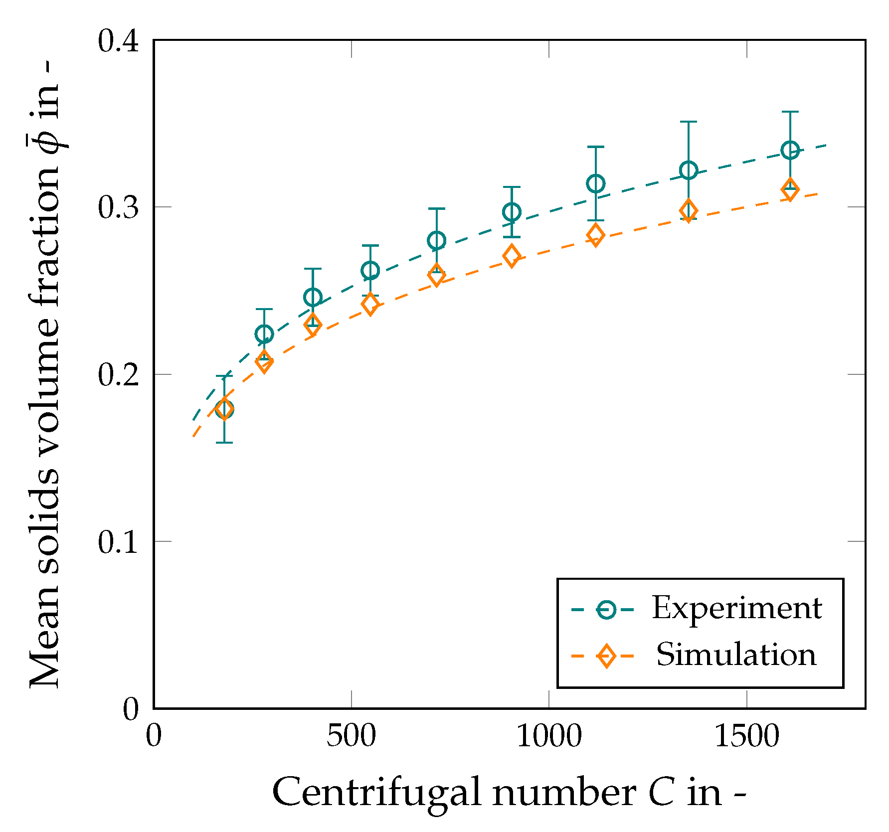
Figure 10.
Solids volume fraction of the sediment at different centrifugal numbers (, , rpm). Comparison of simulation (orange) and experiment (blue).
Figure 10.
Solids volume fraction of the sediment at different centrifugal numbers (, , rpm). Comparison of simulation (orange) and experiment (blue).

Figure 11.
Solids volume fraction of the sediment at different centrifugal numbers (, , ). Comparison of simulation (orange) and experiment (blue).
Figure 11.
Solids volume fraction of the sediment at different centrifugal numbers (, , ). Comparison of simulation (orange) and experiment (blue).

Figure 12.
Relative tangential velocity component parallel to the axis of rotation at and . The gray colored part indicates the sediment.
Figure 12.
Relative tangential velocity component parallel to the axis of rotation at and . The gray colored part indicates the sediment.

Figure 13.
Cuts orthogonal to the axis of rotation of the radial velocity component in the cylindrical part (a), in the inlet section (b), and in the conical part (c) of the decanter centrifuge at and . The gray-colored part indicates the sediment. Positive values point toward the inner wall of the bowl, negative values toward the screw body.
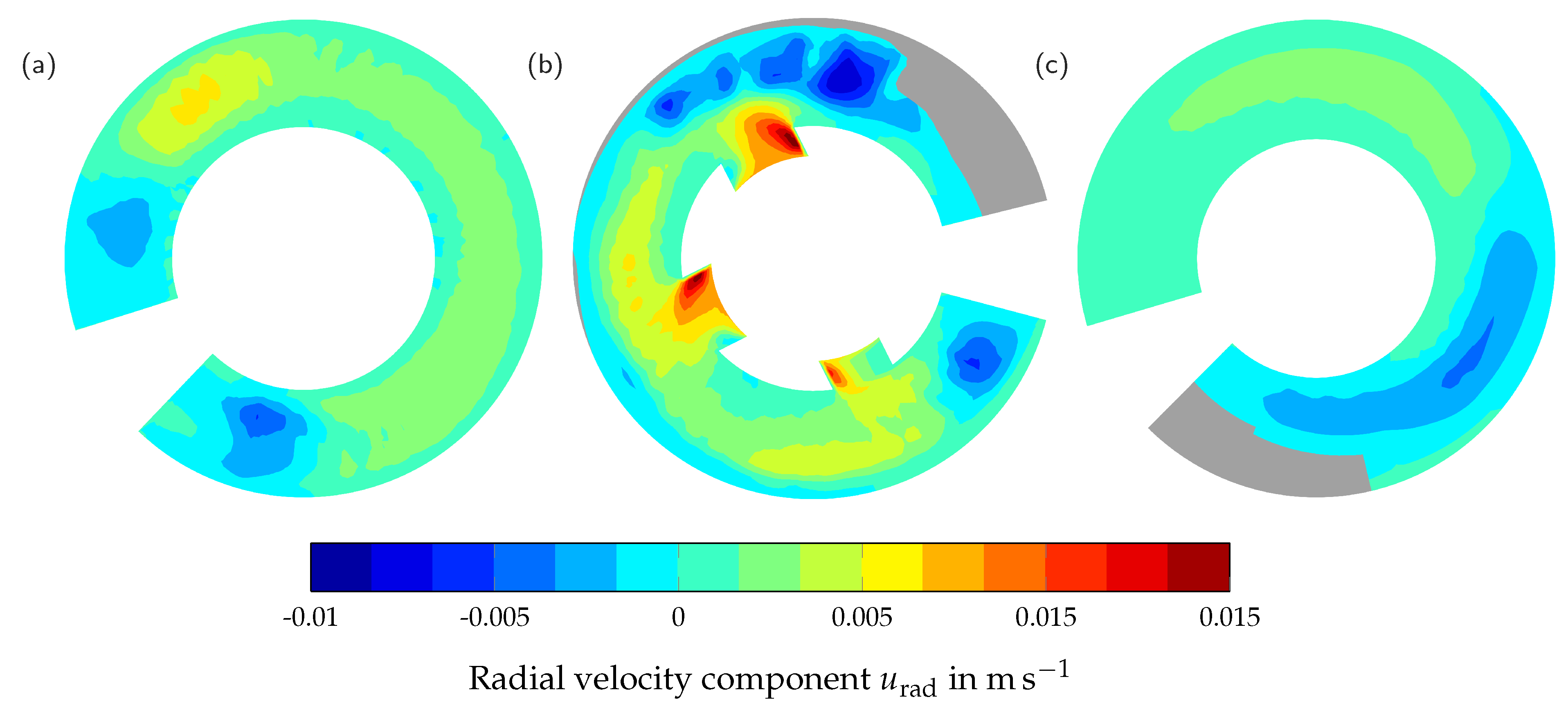
Figure 14.
Cuts orthogonal to the axis of rotation of the axial velocity component in the cylindrical part (a), in the inlet section (b), and in the conical part (c) of the decanter centrifuge at and . The gray-colored part indicates the sediment. Positive values point toward the cone, negative values point toward the weir.


Table 1.
Overview of the used material characteristics.
| Parameter | Symbol | Unit | Kaolin |
|---|---|---|---|
| Particle size | m | 3 | |
| Density of kaolin | kg m−3 | 2600 | |
| Density of water | kg m−3 | 1000 | |
| Gel point | - | ||
| Maximum concentration | - | 1 | |
| Hindered settling parameter | - | 4.65 | |
| Consolidation parameter | Pa | 1.2 | |
| Consolidation parameter | - | 9 | |
| Yield point | Pa | 1 | |
| Consistency | k | m2 s−1 | 0.001 |
| Rheological exponent | - | 1 |
Table 2.
Characteristics of the decanter centrifuge MD80-S.
| Geometry Parameter | Symbol | Unit | Value |
|---|---|---|---|
| Inner radius of the bowl | r | mm | 40 |
| Length of the cylindrical part | mm | 172 | |
| Length of the conical part | mm | 143 | |
| Slenderness ratio | - | - | 3.85 |
| Cone angel | ° | 7 | |
| Pitch | mm | 23 | |
| Flight thickness | mm | 2 | |
| Weir height | mm | 10 |
Table 3.
Boundary conditions of the simulation.
| Inlet | Outlet | Rotating Walls | Stationary Walls | |
|---|---|---|---|---|
| flowRateInletVelocity | zeroGradient | movingWallVelocity | fixedValue | |
| p | fixedFluxPressure | fixedValue | fixedFluxPressure | fixedFluxPressure |
| fixedvalue | zeroGradient | zeroGradient | zeroGradient | |
| zeroGradient | zeroGradient | zeroGradient | zeroGradient | |
| zeroGradient | zeroGradient | zeroGradient | zeroGradient |
Disclaimer/Publisher’s Note: The statements, opinions and data contained in all publications are solely those of the individual author(s) and contributor(s) and not of MDPI and/or the editor(s). MDPI and/or the editor(s) disclaim responsibility for any injury to people or property resulting from any ideas, methods, instructions or products referred to in the content. |
© 2023 by the authors. Licensee MDPI, Basel, Switzerland. This article is an open access article distributed under the terms and conditions of the Creative Commons Attribution (CC BY) license (https://creativecommons.org/licenses/by/4.0/).
Share and Cite
MDPI and ACS Style
Baust, H.K.; Hammerich, S.; König, H.; Nirschl, H.; Gleiß, M. Resolved Simulation of the Clarification and Dewatering in Decanter Centrifuges. Processes 2024, 12, 9. https://doi.org/10.3390/pr12010009
AMA Style
Baust HK, Hammerich S, König H, Nirschl H, Gleiß M. Resolved Simulation of the Clarification and Dewatering in Decanter Centrifuges. Processes. 2024; 12(1):9. https://doi.org/10.3390/pr12010009
Chicago/Turabian StyleBaust, Helene Katharina, Simon Hammerich, Hartmut König, Hermann Nirschl, and Marco Gleiß. 2024. "Resolved Simulation of the Clarification and Dewatering in Decanter Centrifuges" Processes 12, no. 1: 9. https://doi.org/10.3390/pr12010009
Note that from the first issue of 2016, this journal uses article numbers instead of page numbers. See further details here.