Abstract
This study addresses the problem of fault detection in industrial processes by developing a time/frequency feature-driven ensemble learning method. In contrast to the current works based on time domain ensemble learning, this approach adequately integrates the critical frequency domain information. The frequency domain information can be used to effectively enhance the fault detection performance in ensemble learning. Here, the feature ensemble net (FENet) is chosen to capture the time domain feature. The power spectral density (PSD)-based frequency domain feature extraction network can capture the frequency domain features. Bayesian inference can then be used to combine the fault detection results that rely on time/frequency domain features. The simulations of the Tennessee Eastman Process (TEP) demonstrate that the proposed method significantly outperforms traditional methods. The average fault detection rate (FDR) of TEP faults 3, 5, 9, 15, 16, and 21 is 90.63%, much higher than that of 75% by FENet with one feature transformation layer, and those of about 4% by principal component analysis (PCA) and dynamic PCA (DPCA). This research provides a promising framework for more advanced and reliable fault detection in industrial applications.
1. Introduction
Fault detection plays a crucial role in ensuring the safety, reliability, and efficiency of industrial processes. In modern society, as industrial systems become increasingly complex, the early and exact detection of faults—especially incipient ones that develop gradually over time—has become more critical than ever. If the evolving faults remain undetected during the operation of industrial systems, they may lead to severe disruptions, economic losses, and even catastrophic failures, etc. Therefore, there is a growing demand for advanced fault detection technologies capable of the reliable and real-time detection of faults.
Until now, data-driven fault detection has attracted plenty of interest over the past decades. There exist numerous kinds of famous methods like principal component analysis (PCA) [1], partial least square (PLS) [2], and independent component analysis (ICA) [3], etc. While these methods have been effective in detecting faults in certain cases, they have notable limitations. Their reliance on linear assumptions makes them less effective in handling complex, nonlinear industrial processes. Hence, different variants of these methods have been proposed by considering dynamic and nonlinear properties, such as dynamic PCA (DPCA) [4], dynamic PLS (DPLS) [5], kernel PCA (KPCA) [6], and kernel PLS (KPLS) [7], etc. Although these methods can enhance the detection performance, they cannot detect the notable incipient faults 3, 9, and 15 in the Tennessee Eastman Process (TEP), which are characterized by their tiny magnitude and easy contamination by noises or disturbances.
In recent years, the idea of ensemble learning has also been applied to the field of fault detection [8,9,10,11,12,13,14,15,16,17,18,19]. Compared with a single model, ensemble learning improves the accuracy and robustness by integrating the different detection decisions of multiple models. The distributed integrated stack autoencoder performs nicely in nonlinear process monitoring [8]. The AdaBoost algorithm with optimized sampling can detect incipient motor faults [9]. The performance of non-Gaussian process monitoring can be obtained through an improved independent component analysis (ICA) integrated model [10]. Together with Bayesian inference, the enhanced ICA ensemble model improves the accuracy of process monitoring. The integrated learning model based on PCA enhances the monitoring capability of industrial processes [11]. An improved independent component analysis can be used for fault detection in non-Gaussian processes [12]. The integrated KPCA model through local structural analysis can improve the ability to monitor complex processes [13]. The stacked ensemble learning model can significantly improve the performance of fault detection [14]. The deeply integrated forest model shows superior performance in industrial fault classification [15]. A systematic review of ensemble learning-based fault diagnosis is conducted [16]. A model combined with multi-task ensemble learning achieves excellent results in the fault detection of rotary vector retarder [17]. The integrated monitoring model based on depth feature partitioning also improves the detection accuracy of complex systems [18].
Recently, there has also been a series of intriguing studies on ensemble learning-based fault detection. By integrating PCA, a PCA ensemble detector (PCAED) was proposed for detecting TEP faults 3, 9, and 15 [19]. These faults are typically three kinds of incipient faults, which are notably difficult to detect [4,5,6,8,9,10,11,12,13,14,15,16,17,18,19,20]. Based on bootstrap sampling, several PCA detectors were designed to obtain two statistical matrices. A deep framework, namely a feature ensemble net (FENet), can integrate different kinds of detection statistics to achieve superior performance, compared with PCAED. After integrating the detection statistics, the detection feature matrix is obtained and the feature transformation layer is designed with sliding window singular values and PCA as the hidden layer. At the decision level, the detection index is designed based on the statistical properties of singular values. Furthermore, a dense FENet was proposed [20], which can effectively improve the fault detection performance of the original FENet. The idea of FENet was also used to process quality monitoring, which effectively detects faults related to process quality [21].
Note that the abovementioned works only utilize the time domain features inherent to the sample data. Here, the frequency domain features are integrated to effectively enhance the fault detection performance. In contrast to the current works, which are only based on time domain ensemble learning, a time/frequency feature-driven ensemble learning method is proposed. It adequately integrates the critical frequency domain feature inherent in the sample data using the technique of power spectral density (PSD). Here, the FENet is chosen to capture the time domain features, while the PSD-based frequency domain feature extraction network can capture the frequency domain features. Bayesian inference can be used to combine fault detection results from time/frequency domain features. Simulations of TEP sufficiently verify that the frequency domain features effectively achieve better performance in ensemble learning, providing improved detection accuracy, especially on TEP faults 3, 9, and 15. The main contributions of the proposed method are listed as follows:
- (1)
- A time/frequency feature-driven ensemble learning method is proposed to address the problem of fault detection in industrial processes. The integration of the frequency-domain information can effectively enhance the fault detection performance.
- (2)
- Compared with time domain (namely FENet with only one feature transformation layer), and PCA, the proposed method can effectively detect incipient faults 3, 9, and 15 in TEP, which are notably difficult to detect in the field of fault detection [4,5,6,8,9,10,11,12,13,14,15,16,17,18,19,20]. Until now, there have been scare works that have successfully detected these incipient faults.
The rest of the paper is organized as follows: Section 2 provides a formulation of the problem. In Section 3, the idea of FENet is briefly introduced. In Section 4, the proposed time/frequency feature-driven ensemble learning is developed in detail, including the detailed description on extracting frequency domain features and the Bayesian inference-based ensemble learning. In Section 5, TEP is chosen as an example to demonstrate the effectiveness of the proposed method. Section 6 gives a discussion of the problem of incipient faults and a brief survey of the findings. Finally, the conclusion is given in the last section.
2. Problem Formulation
The task of fault detection in complex industrial processes has been widely considered in the past decades. Although a variety of data-driven fault detection methods have been proposed, only a few methods can effectively detect the incipient TEP faults 3, 9, and 15, which are notably difficult in the field of fault detection, due to the tiny amplitude and the easy contamination by noise or disturbance.
For incipient faults, ensemble learning may be a possible way to obtain better performance, compared with single model-based detection. Decisions from different classes of fault detectors can be fused, which rely heavily on the performance of each detector. However, ensemble learning-based works to detect incipient faults such as TEP faults 3, 9, and 15 are scarce.
In this paper, the problem of fault detection is considered in the framework of ensemble learning. Compared with the current ensemble learning works, an ensemble learning approach is developed by combing time domain and frequency domain features on sample data. The key interest is to introduce frequency domain features into ensemble learning, which significantly outperforms traditional methods, providing improved detection accuracy, especially on TEP faults 3, 9, and 15.
3. Time Domain Feature Ensemble Net (FENet)
Here, the time domain FENet is introduced [22], which consists of an input feature, feature transformation, an output feature, and decision layers. Denote as the process measurements, where is the number of sensors. If samples are collected under normal conditions, the training data are , where is normalized to the sample mean and standard deviation. Given and a detector, a mapping from to the detection statistics is donated as . Here, is described by formulas like , where the projection operator corresponds to the detector.
At the input feature layer, for , the detectors result in a feature vector:
where represents the detection statistics on sample for the -th detector. Thus, based on Equation (1), the input feature matrix is denoted as follows [22]:
At the feature transformation layer, the feature matrix is subjected to a series of transformations through layers. For layer , a sliding window of size is applied to the feature matrix like Equation (2), resulting in a submatrix for each window :
where and is the combination of columns selected for transformation. Next, singular value decomposition (SVD) is applied to as follows:
where , , and are the left singular matrix, diagonal matrix of singular values, and right singular matrix, respectively. Singular values in are then used to calculate the and statistics by PCA for each window :
where is the covariance matrix of , and is the mean vector of singular values. These statistics are finally stacked to form a new feature matrix for the next layer:
All feature matrices generated at the last (th) transformer layer can be fully stacked into a large matrix, . For , the feature matrix in the output feature layer is equal to that in the input feature layer.
At the decision layer, a fully sliding window is applied to matrix to extract a submatrix for sample :
where . After scaling to , is decomposed into
For sample , the detection index is computed as follows [22]:
where is the vector of singular values, and are the mean and standard deviation of , respectively. The control limit can be calculated with a given significance level using the kernel density estimation (KDE). If exceeds , a fault is detected at sample .
4. Time/Frequency Feature-Driven Ensemble Learning
Note that time domain FENet can achieve a better performance if the number of feature transformation layers is sufficiently large [22]. However, there exist two shortcomings inherent in FENet: (1) the computation cost increases largely with the increasing number of the transformation layers due to a large amount of the computation of SVDs; (2) the performance is relatively worse if there exists only one transformation layer. Note that the FDRs of TEP faults 15, 16, and 21 by FENet with only one feature transformation layer (namely, ) are only 61.60%, 72.20%, and 72.60%, respectively [22]. This is obviously worse than the FDRs of TEP’s other faults.
To address these two shortcomings of , an efficient resolution is to integrate the time/frequency domain features through ensemble learning. Even using only one transformation layer in can effectively increase the detection performance, especially for TEP faults 3, 9, and 15.
In this paper, an ensemble learning driven by the time/frequency feature is proposed to improve the detection performance of TEP fault detection. is selected for capturing time domain features and detecting faults. In addition, the frequency domain feature extraction network based on PSD can obtain the frequency domain feature of sample data. Finally, the fault detection results from time/frequency domain features are combined with Bayesian inference.
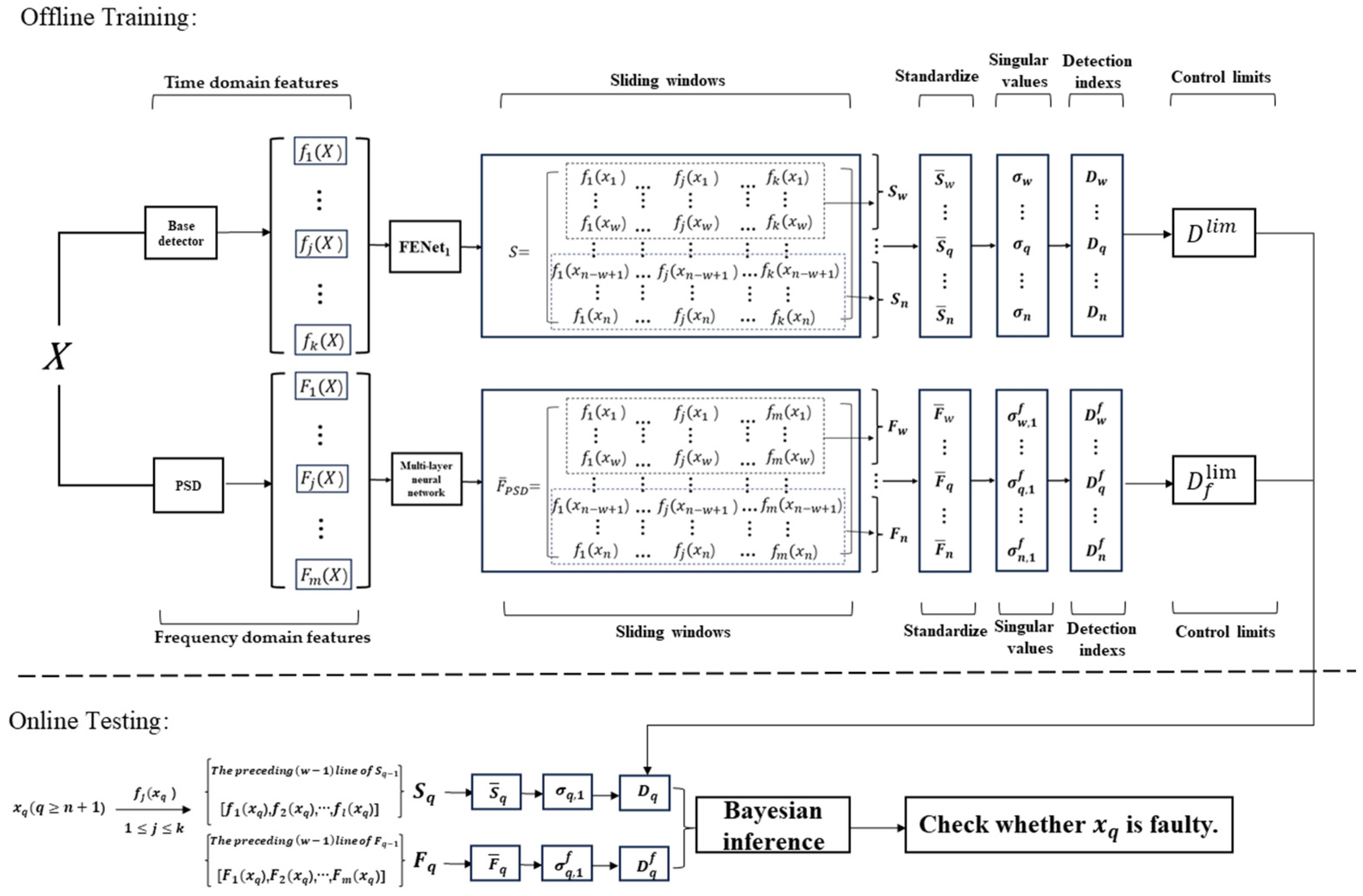
The detailed scheme of time/frequency feature-driven ensemble learning is shown in Figure 1. As stated above, there are two additional key components in time/frequency feature-driven ensemble learning compared with time domain . The first is to introduce a PSD-based feature extraction network in the frequency domain, which provides an alternative way for designing fault detectors. The second is Bayesian inference, which combines fault detection results based on time/frequency domain features. In Figure 1, , represent the time/frequence domain feature vectors on , respectively.
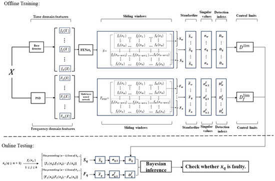
Figure 1.
Overall diagram of time/frequency feature driven ensemble learning.
4.1. Frequency Domain Feature Extraction Network
Here, a frequency domain feature extraction network is developed to capture the frequency domain feature inherent in sample for . This kind of network performs two main tasks: one is to use the power spectral density (PSD) to obtain the SVD-based frequency domain feature matrix, and the other is to transform the frequency domain feature matrix using a multi-layer neural network.
For the SVD-based frequency domain feature matrix, the PSD can be first obtained using the Welch method [23]. Here, the time series is divided into multiple overlapping segments. Each segment has a length of N, and the overlap length between adjacent segments is D. This design of overlapping segments reduces variance in the spectral estimation while improving spectral resolution. A window function w[i] is applied to each segment, such as the Hanning window, defined by
The discrete Fourier transform (DFT) is then performed on each windowed segment to transform it into the frequency domain. The DFT of each segment is referred to as the periodogram of that segment. The periodogram of all segments is averaged to estimate the PSD. Thus, the PSD estimated by the Welch method is given by
here, M is the number of segments, U is the normalization factor to ensure that the estimated energy matches the sample, and denotes the number of frequency bins after applying the DFT to each window segment. Note that each row of corresponds to the -th feature, which represents the PSD value at a particular frequency at a particular segment.
In order to extract key frequency domain features, is first normalized into , represented by
where and represent the mean and standard deviation of feature j, respectively.
For a predefined window size W and step size S, is divided into many small matrices , and the SVD is performed:
with a left singular vector matrix U, a singular value matrix , and a right singular vector matrix . The top singular values from different window segments are then combined to form the final comprehensive frequency domain feature matrix . Therefore, can be represented as the aggregation of these :
where denotes the number of window segments.
For transforming the frequency domain feature matrix , a multi-layer neural network is used. In each layer , a non-linear function (⋅) is applied to to capture the deep frequency domain features. The final output feature is represented as follows:
For , a fully sliding window is applied to extract a submatrix for sample :
where . After scaling to , is decomposed into
Using singular values of , the detection index is computed as follows:
where is the vector of singular values from ,; and are the mean and standard deviation of respectively. The control limit is calculated with a given significance level using KDE [24]. If exceeds the threshold , a fault is detected at sample .
4.2. Bayesian Inference
Here, Bayesian inference is used to combine the fault detection results based on time/frequency domain features. Bayesian inference is fundamentally about updating the probability of a fault based on prior knowledge and samples. For the proposed time/frequency feature-driven ensemble learning, there are two detectors to detect faults. One is the time domain , and the other is the frequency domain feature extraction network, as described above. Here, the statistical features of training and testing data are represented as matrices and , where and denote the number of training and testing samples, respectively.
For each training sample and detector , the likelihood functions under normal conditions for and under faulty conditions are , given by the following:
where is a tuning parameter, and corresponds to the control limit of detector . As stated above, and . The overall likelihood is a combination of the prior probabilities for abnormal and normal conditions:
where is also a tuning parameter.
Using Bayes’ theorem, the posterior probability that a sample belongs to a faulty state is calculated as follows:
From Equation (24), the final statistic is a weighted posterior probability for each detector. The weight is determined by the relative magnitude of the likelihood function under faulty conditions, expressed as follows:
The final statistic is then the sum of the weighted posterior probabilities for two detectors:
By integrating the detection results of in the time domain and the feature extraction network in the frequency domain, the Bayesian inference effectively updates the posterior probability of faults of the sample . This fusion can lead to more accurate fault detection.
4.3. Algorithms
For time/frequency feature-driven ensemble learning, two offline algorithms and one online algorithm are required. Algorithm 1 gives the detailed off-line training procedure of FENet in time domain. In particular, the method utilizes time domain to obtain detection result based on time domain features. Here, . Algorithm 2 presents the off-line training process of the frequency domain feature extraction network. After two off-line training algorithms, Algorithm 3 gives the online testing process of time/frequency feature-driven ensemble learning.
| Algorithm 1: Time domain FENet (Off-line Training) |
| Input: DataSet—training dataset, number of base detectors, window size for sliding windows, maximum feature transformation layers, significance level; Output: the control limit, for to —the set of base detectors, the structure of time domain FENet; 1. Initialize detectors for to by ; 2. Obtain (2); 3. If , then 4. Assign = and skip to step 12; 5. else 6. Set = ; 7. for = 0, 1, 2, …, − 1 do 8. Obtain by (3)–(7); 9. end for 10.end if 11. Obtain ; 12. for do 13. Extract (8) from ; 14. Normalize as (9); 15. Compute of ; 16. end for 17. Calculate (10); 18. Calculate with the significance level . |
| Algorithm 2: Frequency Domain Feature Extraction Network (Off-line Training) |
| Input: frequency-domain sample, segment length, overlap length, window function, size of sliding windows; Output: the control limit, the structure of frequency domain feature extraction network; 1: Divide into segments of length with overlap ; 2: Apply (11) to each segment; 3: for segment length and overlap do 4: Compute DFT; 5: Store periodogram of the segment; 6: end for 7: Average periodograms to estimate PSD, denoted as (12); 8: Normalize to (13); 9: for window size do 10: Divide into (14); 11: Perform SVD on ; 12: Extract first singular values ; 13: Normalize to form ; 14: end for 15: Combine features from different scales to form (15); 16: Process through multi-layer neural network to obtain (16); 17: for do 18. Extract (17) from ; 19. Normalize as (18); 20. Compute of ; 21. end for 22: Calculate (19); 23. Calculate with the significance level . |
| Algorithm 3: Time/Frequency Feature Driven Ensemble Learning (Online Testing) |
| Input: —a new sample, —the control limits, the structure of time domain FENet, the structure of frequency domain feature extraction network; Output: the status (normal or faulty) of ; % The update of time domain feature 1. For , obtain (2); 2. If , then 3. Assign ; 4. else 5. Set ; 6. Update using and (3)–(7); 7. For each layer 8. Calculate ; 9. End for 10. End If 11. Update (8); 12. Normalize to get (9); 13. Calculate singular values of ; 14. Calculate time-domain decision using (10); 15. Obtain the time domain decision on using ; % The update of frequency domain feature 16. For , compute the normalized PSD (12); 17. If , then 18. Assign (13); 19. else 20. Set ; 21. Update using and (14)–(16); 22. For each layer 23. Calculate using ; 24. End for 25. End If 26. Update (17); 27. Normalize to get (18); 28. Calculate singular values of ; 29. Calculate frequency-domain decision using (19); 30. Obtain the frequency domain decision on using ; % Bayesian inference 31. Decide the status of using Bayesian inference (20–25); 32. Return the status of (normal or fault). |
5. Simulations
In this section, the proposed ensemble learning method is verified by the famous benchmark process TEP, which is a highly nonlinear and dynamic process [25]. It is a chemical plant simulation developed by Downs and Vogel of the Eastman Chemical Company [26], and has been widely used to verify the effectiveness of fault detection methods [27]. TEP consists of five main units, namely reactor, separator, stripper, condenser, and compressor. TEP has 53 observed variables, including 22 continuous variables, 19 process variables and 12 operational variables. The 33 variables include 22 continuous variables XMEAS (1)–XMEAS (22) and 11 operational variables XMV (1)–XMV (11), where XMEAS and XMV stand for the abbreviations for ‘measurement’ and ‘measurement variable’, respectively. TEP contains 21 types of faults, among which fault 3 is a step fault, fault 9 is a random variable fault, and fault 15 is a valve sticking fault. These three types of faults are widely considered to be typical incipient faults. Figure 2 shows the system structure of TEP. Table 1 (the second column) gives a detailed description of 21 types of faults.
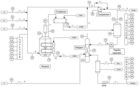
Figure 2.
The system structure of TEP [27].
A closed-loop version of the TEP [28] was used to generate simulation data, available at http://depts.Washington.edu/control/LARRY/TE/download.html (accessed on 22 May 2022). The simulation time for the training dataset and the test dataset were set to 200 h, respectively, and the sampling time was three min. In each test dataset, a fault was introduced after 100 h of simulation. With the exception of fault 6, 4000 training samples and 4000 test faulty samples are obtained for each fault. Note that Fault 0 is a normal dataset, and the last 2000 sampling instants in each testing dataset were calculated to obtain the fault detection rate (FDR). This implies that the FDR of fault 0 indicates the false alarm rate (FAR) of normal data.
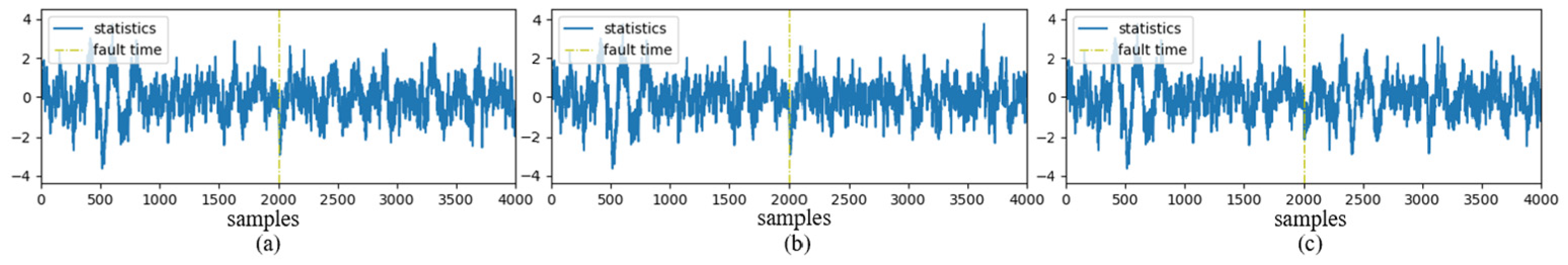
Note that TEP faults 3, 9, and 15 are notably difficult to detect in the field of fault detection [4,5,6,8,9,10,11,12,13,14,15,16,17,18,19,20]. The curves of faults 3, 9, and 15 are shown in Figure 3. Due to their tiny magnitude and susceptibility to contamination by noise or interference, there is virtually no difference between normal and faulty samples. Here, the proposed method can effectively detect these incipient faults.
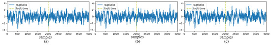
Figure 3.
Time series curves for faults. (a) Fault 3; (b) Fault 9; (c) Fault 15.
In the simulations, the training and test data are first normalized to the sample mean and standard deviation. For time domain , simple detectors (PCA, DPCA, MD) were selected as basic detectors, where the mapping can be described by , like the formulations given in Table 1 in [22]. Three variants of Mahalanobis Distance (MD) are also used as basic detectors, namely , , and , whose input variables are set as 33 variables [XMEAS (1–22) and XMV (1–11)], 22 continuous process variables [XMEAS (1–22), and 11 manipulated variables [XMV(1–11)], respectively. For PCA, DPCA, and MD, the number of basic detectors is . The width of the sliding-window patches is . The significance level of each detector is , and the corresponding control limit is determined by KDE. It can be seen that the FDRs of TEP faults 15, 16, and 21 by time domain are only 61.60%, 72.20%, and 72.60%, respectively. Although it is higher than other well-known ensemble learning strategies such as voting, averaging, and Bayesian inference for the above basis detectors, it is relatively poor compared with the FDRs of other faults in TEP.
For a frequency domain feature extraction network, a multi-layer neural network is used to further extract features from PSD-based frequency domain feature matrix . Here, the number of nodes in the input layer corresponds to the dimensionality of matrix . The network consists of three hidden layers, equipped with 128, 64, and 32 neurons, respectively. For each hidden layer, a rectified linear unit (ReLU) activation function is applied to introduce nonlinearity. In addition, there are two nodes in the output layer, meaning the normal/faulty states of the sample, where the activation function is chosen as the soft maximum (Softmax) function. In this simulation, parameter n (total number of samples) is set to 4000, parameter N (length of each segment) is set to 256, and parameter D (length of overlap between segments) is set to 32.
In this paper, a time/frequency feature-driven ensemble learning is proposed to increase the detection performance. Time domain and frequency domain feature extraction network run in parallel. After the time/frequency domain fault detection decisions, the fault detection results from these two fault detectors can be combined using Bayesian inference. In this simulation, parameters γ and η are chosen to be 0.2 and 0.01, respectively.
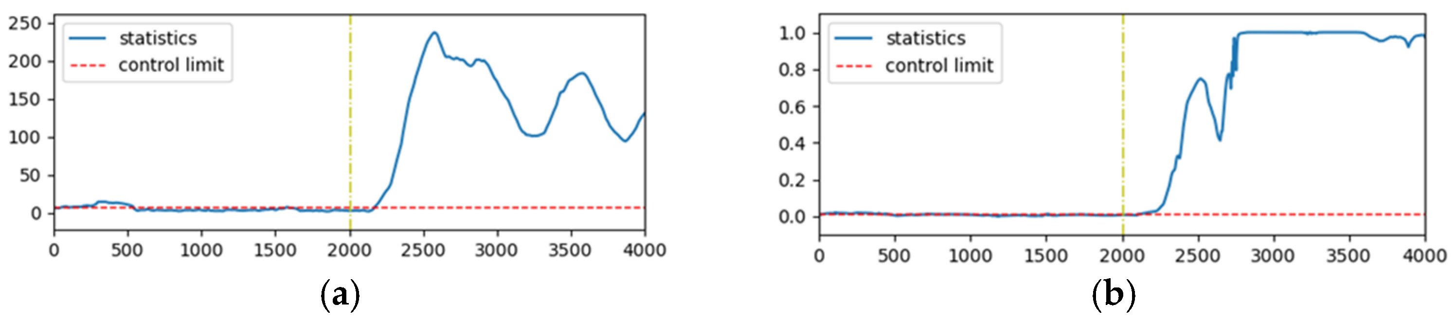
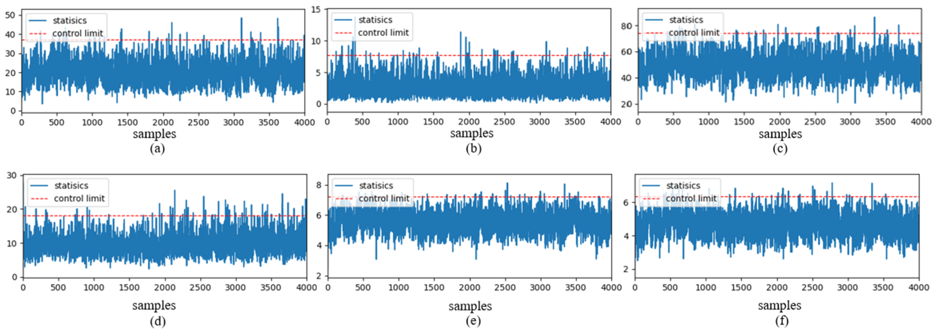
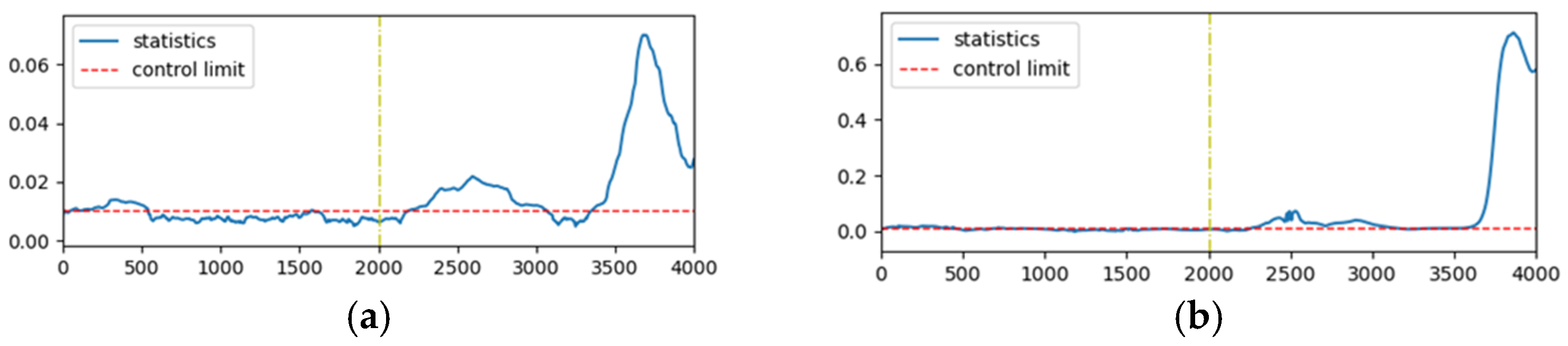
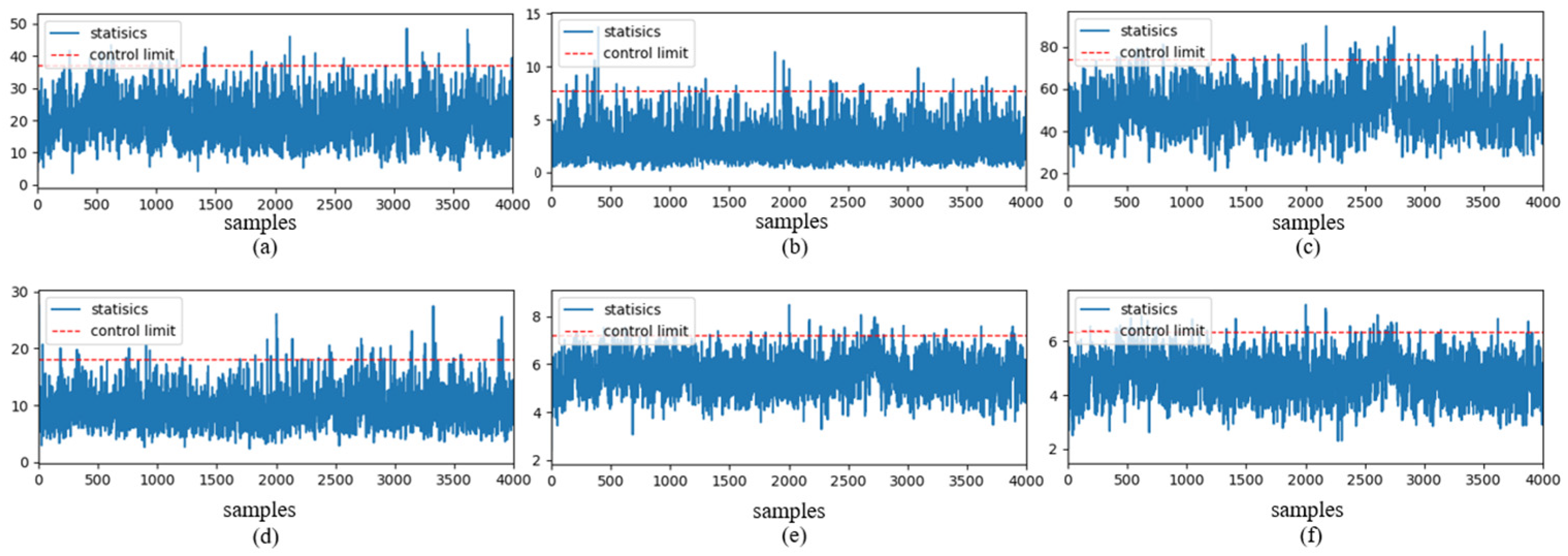
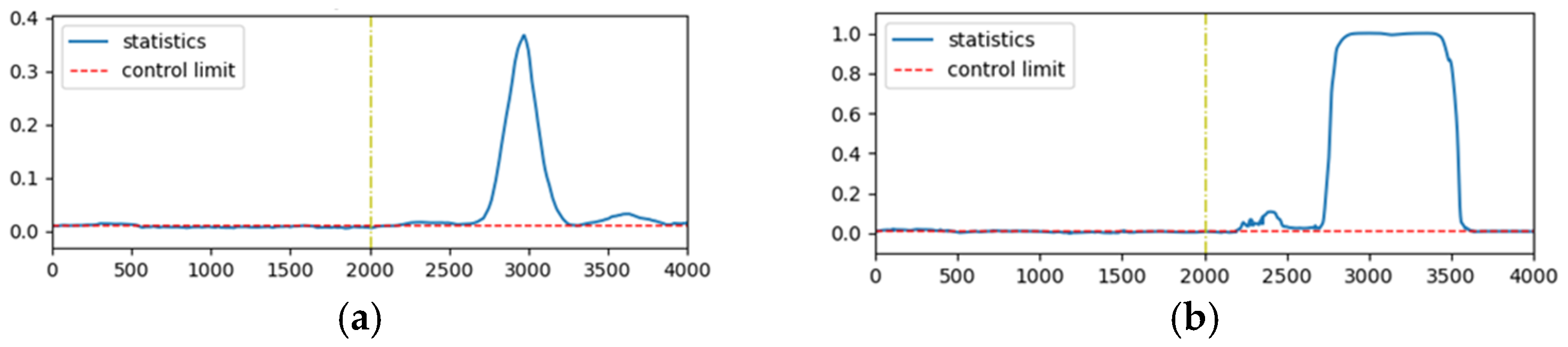
Figure 4, Figure 5, Figure 6 and Figure 7 show the performance curves of incipient faults 3 and 15 in TEP using different detection methods. Since faults 3 and 15 are too tiny, traditional methods such as PCA, DPCA, and MD cannot detect these two faults. From Figure 4 and Figure 6, the performance of traditional methods is low. Although time domain FENet1 can achieve the FDR of 93.25% for fault 3 (Table 1), the proposed method can achieve a higher FDR, namely 94.80%. For incipient fault 15, time domain FENet1 only obtains the FDR of 61.60%. However, the proposed method can achieve the FDR of 84.40%. In addition, the performance of fault 5 is given in Figure 8 and Figure 9. Although fault 5 is not an incipient fault, the FDRs of PCA, DPCA, and MD are less than 4%, while time domain FENet1 only achieves the FDR of 55.65%. In contrast, the proposed method achieves an FDR of 91.55%, considerably higher than those of the contrasting methods.
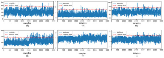
Figure 4.
Detection performance of fault 3 in TEP. (a) PCA (); (b) PCA (); (c) DPCA (); (d) DPCA (); (e) (); (f) ().
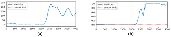
Figure 5.
Detection performance of fault 3 in TEP. (a) Time domain FENet1; (b) The proposed method.
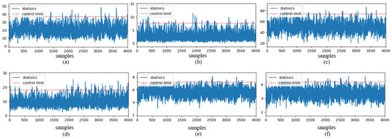
Figure 6.
Detection performance of fault 15 in TEP. (a) PCA (); (b) PCA (); (c) DPCA (); (d) DPCA (); (e) (); (f) ().
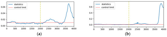
Figure 7.
Detection performance of fault 15 in TEP. (a) Time domain FENet1; (b) The proposed method.

Figure 8.
Detection performance of fault 5 in TEP. (a) PCA (); (b) PCA (); (c) DPCA (); (d) DPCA (); (e) (); (f) ().
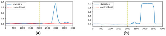
Figure 9.
Detection performance of fault 5 in TEP. (a) Time domain FENet1; (b) The proposed method.
The detailed performance on all kinds of faults in TEP is given in Table 1. Obviously, PCA, DPCA, MD, FENet1, and the proposed method exhibit different performances. PCA and DPCA show very high FDRs for certain fault types. For PCA and DPCA, the FDRs of fault 6 (step) and fault 7 (step) both reach 100.00%. However, for random variation and unknown types of faults (e.g., fault 3 and fault 16), the FDRs of PCA and DPCA drop significantly, down to 5.70% and 1.80%, respectively. As for MD, while it shows high detection capability for certain fault types (e.g., faults 1, 2, 4, and 6), it performs poorly when detecting random variation faults (e.g., faults 9 and 12). This indicates that MD’s sensitivity to faults varies greatly under different conditions. In contrast, FENet1 demonstrates relatively stable detection performance across most fault types, with an FDR close to 99.85% in step faults. Since PCA and DPCA can reach 100% for faults 6 and 7, the FDRs of FENet1 also reach 100% since FENet1 is actually a kind of ensemble learning of PCA and DPCA. However, for FENet1, the FDRs of TEP faults 5, 15, 16, and 21 are only 55.65%, 61.60%, 72.20%, and 72.60%, respectively. Although it is higher than PCA, DPCA, MD, and other famous ensemble learning strategies such as voting, averaging, and Bayesian inference, it is relatively worse, compared with the FDRs of other faults in TEP.
As shown in Table 1, PCA, DPCA, MD, and FENet1 show the similar/slightly better performance than the proposed method when detecting faults 1, 2, 4, 6–8, 10–14, and 17–20. However, when detecting faults 3, 5, 9, 15, 16, and 21, the proposed method shows the bast performance. The average FDR of these faults is 90.63%, much higher than that of 75% by FENet1, and those of about 4% by PCA and DPCA. In fact, incipient faults 3, 9, and 15 are extremely difficult to detect in the field of fault detection [4,5,6,8,9,10,11,12,13,14,15,16,17,18,19,20]. Even for faults 5, 16, and 21, which are not incipient, PCA, DPCA, and MD are indeed ineffective. For FENet1, the FDRs of these faults are less than 72.60%, much lower than those of the proposed method. Since the proposed method is actually the ensemble learning of FENet1 and the frequency domain feature extraction network, the FDRs of faults 6 and 7 are also 100%. As stated above, integrating frequency features with Bayesian inference significantly improves FDRs, especially for incipient and random variation faults.

Table 1.
FDRs () of PCA, DPCA, MD, FENET1, and the proposed method.
Table 1.
FDRs () of PCA, DPCA, MD, FENET1, and the proposed method.
| Fault | Type | PCA | DPCA | MD | FENet1 | The Proposed Method | ||
|---|---|---|---|---|---|---|---|---|
| MD1 | MD2 | MD3 | ||||||
| 0 | Normal | 1.70 | 2.10 | 1.05 | 0.70 | 0.70 | 1.40 | 0.1 |
| 1 | Step | 99.95 | 99.95 | 99.95 | 99.90 | 99.90 | 99.85 | 99.85 |
| 2 | Step | 99.90 | 99.80 | 99.85 | 99.65 | 99.65 | 99.50 | 99.45 |
| 3 | Step | 5.70 | 10.25 | 2.65 | 2.60 | 1.05 | 93.25 | 94.80 |
| 4 | Step | 99.95 | 99.95 | 99.95 | 2.00 | 99.95 | 99.95 | 99.95 |
| 5 | Step | 3.35 | 4.00 | 2.05 | 1.35 | 2.00 | 55.65 | 91.55 |
| 6 | Step | 100.00 | 100.00 | 100.00 | 100.00 | 100.00 | 100.00 | 100.00 |
| 7 | Step | 100.00 | 100.00 | 100.00 | 3.25 | 100.00 | 100.00 | 100.00 |
| 8 | Random variation | 99.65 | 99.65 | 99.65 | 99.65 | 99.60 | 99.50 | 99.50 |
| 9 | Random variation | 7.70 | 12.85 | 5.55 | 3.70 | 1.60 | 94.70 | 95.00 |
| 10 | Random variation | 93.55 | 95.30 | 95.50 | 91.55 | 76.80 | 98.75 | 98.75 |
| 11 | Random variation | 98.70 | 99.45 | 98.95 | 90.20 | 94.45 | 99.90 | 99.90 |
| 12 | Random variation | 46.50 | 61.50 | 51.35 | 46.25 | 22.70 | 99.10 | 99.05 |
| 13 | Slow drift | 97.65 | 97.55 | 97.45 | 97.55 | 97.45 | 97.20 | 97.15 |
| 14 | Sticking | 99.90 | 99.90 | 99.90 | 99.90 | 87.10 | 99.80 | 99.80 |
| 15 | Sticking | 3.05 | 2.50 | 1.25 | 0.90 | 0.80 | 61.60 | 84.40 |
| 16 | Unknown | 1.80 | 2.40 | 0.45 | 0.65 | 0.65 | 72.20 | 89.10 |
| 17 | Unknown | 99.10 | 99.15 | 99.15 | 99.15 | 88.40 | 99.00 | 99.00 |
| 18 | Unknown | 87.05 | 93.20 | 87.10 | 83.35 | 14.85 | 97.80 | 97.80 |
| 19 | Unknown | 99.90 | 99.85 | 99.90 | 58.85 | 99.90 | 99.75 | 99.75 |
| 20 | Unknown | 99.30 | 99.30 | 99.40 | 99.45 | 98.70 | 99.30 | 99.20 |
| 21 | Constant position | 2.90 | 3.65 | 1.65 | 1.45 | 1.60 | 72.60 | 88.90 |
| Average * | - | 4.08 | 5.94 | 2.27 | 1.78 | 1.28 | 75.00 | 90.63 |
* The average FDR of faults 3, 5, 9, 15, 16, and 21.
In summary, the time/frequency feature-driven ensemble learning significantly improves the detection rates by integrating time domain and frequency domain information. Simulation results demonstrate that the proposed method has significant advantages in enhancing the robustness and accuracy of fault detection in complex industrial processes, providing a reliable theoretical and practical foundation for further engineering applications.
6. Discussion
Because no physical model is required, data-driven fault detection is a research topic in the field of fault detection in dynamic processes. From PCA and PLS to various variants, different properties are considered to solve the fault detection problem. Although fault detection has come a long way, the detection of incipient faults is still difficult. Fault 3, fault 9, and fault 15 are typical incipient faults, which are difficult to detect because of their tiny amplitude and they are easy to be polluted by noise or interference. Most data-driven approaches are not effective at detecting these incipient faults.
Generally speaking, data-driven fault detection methods are divided into time domain and frequency domain methods. PCA and PLS fall into the former category, while PSD-based methods fall into the latter. Due to the restriction of data-driven methods for detect incipient faults, the idea of ensemble learning is also used for fault detection. Although ensemble learning can effectively improve the detection performance, it is still a difficult task for most ensemble learning methods to detect TEP faults 3, 9, and 15. For now, only time domain FENet shows excellent ensemble learning performance in dealing with incipient faults including the above faults if the number of feature transformation layers is sufficiently large [22].
However, with the increase in the number of transformation layers, the computational cost of time domain FENet will increase greatly with the increase in the computation amount of SVD. In addition, the performance of time domain FENET1 is relatively poor. The FDRs of TEP faults 15, 16, and 21 by time domain FENET1 are only 61.60%, 72.20%, and 72.60%, respectively. The main contribution of the proposed method is the integration of time domain/frequency-domain features into ensemble learning. The proposed method can effectively detect incipient faults 3, 9, and 15 in TEP, and its performance is better than that of time domain FENET1.
It is worth noting that the proposed ensemble learning method is suitable for stationary processes. However, numerous realistic industrial processes are non-stationary. Is it possible to design ensemble learning method to detect incipient faults? Does frequency domain information help improve the detection performance of non-stationary processes? These problems deserve further study in the future.
7. Conclusions
Since the 1990s, TEP 3, 9, and 15 faults, as typical early faults, have been significantly more difficult to detect in the fault detection field. Even using the idea of ensemble learning, it is difficult to successfully detect these incipient faults. Most data-driven fault detection methods exhibit poor performance in detecting these incipient faults. In this paper, a time/frequency feature-driven ensemble learning is proposed to resolve the detection problem of incipient faults 3, 9, and 15 in TEP. The new feature of this method is that the frequency domain features are integrated into ensemble learning. The time domain FENET1 and the frequency main feature extraction network based on PSD are run in parallel, and the detection results of time-frequency domain information are combined by Bayesian inference. Using frequency domain features, the detection performance is greatly improved. Take TEP fault 15 as an example, the proposed method is obviously superior to the traditional PCA, DPCA, and time domain FENET1. This research shows the superiority of the ensemble of time/frequency domain feature. However, this method mainly solves the problem of fault detection in stationary processes. Therefore, how to use frequency domain characteristics to improve the detection performance of non-stationary processes will be further considered.
Author Contributions
Conceptualization, methodology, software, validation, formal analysis, Y.M., Z.L. and M.C.; investigation, M.C.; resources, data curation, Y.M. and Z.L.; writing—original draft preparation, writing—review and editing, Y.M., Z.L. and M.C.; visualization, supervision, project administration, M.C.; funding acquisition, M.C. All authors have read and agreed to the published version of the manuscript.
Funding
This research was supported in part by the National Natural Science Foundation of China under Grant 62373213, and in part by Science Foundation of China University of Petroleum, Beijing (No. 2462024YJRC0006).
Data Availability Statement
The data are available from the corresponding author on reasonable request.
Conflicts of Interest
The authors declare no conflicts of interest.
References
- Qin, S.J. Statistical process monitoring: Basics and beyond. J. Chemom. 2003, 17, 480–502. [Google Scholar] [CrossRef]
- Geladi, P.; Kowalski, B.R. Partial least-squares regression: A tutorial. Anal. Chim. Acta 1986, 185, 1–17. [Google Scholar] [CrossRef]
- Lee, J.; Yoo, C.; Lee, I. Statistical process monitoring with independent component analysis. J. Process Control 2004, 14, 467–485. [Google Scholar] [CrossRef]
- Ku, W.; Storer, R.H.; Georgakis, C. Disturbance detection and isolation by dynamic principal component analysis. Chemom. Intell. Lab. Syst. 1995, 30, 179–196. [Google Scholar] [CrossRef]
- Kaspar, M.H.; Ray, W.H. Dynamic PLS modelling for process control. Chem. Eng. Sci. 1993, 48, 3447–3461. [Google Scholar] [CrossRef]
- Lee, J.; Yoo, C.; Choi, S.W.; Lee, I.; Lee, C.B. Nonlinear process monitoring using kernel principal component analysis. Chem. Eng. Sci. 2004, 59, 223–234. [Google Scholar] [CrossRef]
- Rosipal, R.; Trejo, L.J. Kernel partial least squares regression in reproducing kernel Hilbert space. J. Mach. Learn. Res. 2001, 2, 97–123. [Google Scholar]
- Li, Z.; Tian, L.; Jiang, Q.; Zhang, H. Distributed-ensemble stacked autoencoder model for non-linear process monitoring. Inf. Sci. 2020, 542, 302–316. [Google Scholar] [CrossRef]
- Martin-Diaz, I.; Morinigo-Sotelo, D.; Duque-Perez, O.; de la Rosa, J.; Garcia-Perez, A. Early fault detection in induction motors using AdaBoost with imbalanced small data and optimized sampling. IEEE Trans. Ind. Appl. 2017, 53, 3066–3075. [Google Scholar] [CrossRef]
- Ge, Z.; Song, Z. Performance-driven ensemble learning ICA model for improved non-Gaussian process monitoring. Chemom. Intell. Lab. Syst. 2013, 123, 1–8. [Google Scholar] [CrossRef]
- Li, Z.; Yan, X. Ensemble learning model based on selected diverse principal component analysis models for process monitoring. J. Chemom. 2018, 32, e3010. [Google Scholar] [CrossRef]
- Tong, C.; Lan, T.; Shi, X. Ensemble modified independent component analysis for enhanced non-Gaussian process monitoring. Control Eng. Pract. 2017, 58, 34–41. [Google Scholar] [CrossRef]
- Cui, P.; Zhan, C.; Yang, Y. Improved nonlinear process monitoring based on ensemble KPCA with local structure analysis. Chem. Eng. Res. Des. 2019, 142, 355–368. [Google Scholar] [CrossRef]
- Li, G.; Zheng, Y.; Liu, J.; Wang, M. An improved stacking ensemble learning-based sensor fault detection method for building energy systems using fault-discrimination information. J. Build. Eng. 2021, 43, 102812. [Google Scholar] [CrossRef]
- Liu, Y.; Ge, Z. Deep ensemble forests for industrial fault classification. IFAC J. Syst. Control 2019, 10, 100071. [Google Scholar] [CrossRef]
- Mian, Z.; Deng, X.; Dong, X.; Tian, Y.; Cao, T.; Chen, K.; Al Jaber, T. A literature review of fault diagnosis based on ensemble learning. Eng. Appl. Artif. Intell. 2024, 127 Pt B, 107357. [Google Scholar] [CrossRef]
- Wang, H.; Wang, S.; Yang, R.; Xiang, J. A numerical simulation enhanced multi-task integrated learning network for fault detection in rotation vector reducers. Mech. Syst. Signal Process. 2024, 217, 111525. [Google Scholar] [CrossRef]
- Li, Z.; Tian, L.; Yan, X. Ensemble monitoring model based on multi-subspace partition of deep features. IEEE Access 2023, 11, 128911–128922. [Google Scholar] [CrossRef]
- Liu, D.; Shang, J.; Chen, M. Principal component analysis-based ensemble detector for incipient faults in dynamic processes. IEEE Trans. Ind. Inform. 2021, 17, 5391–5401. [Google Scholar] [CrossRef]
- Wang, M.; Cheng, F.; Chen, K.; Qiu, G.; Cheng, Y.; Chen, M. Incipient fault detection based on dense ensemble net. Neurocomputing 2024, 601, 128211. [Google Scholar] [CrossRef]
- Wang, M.; Xie, M.; Wang, Y.; Chen, M. A deep quality monitoring network for quality-related incipient faults. IEEE Trans. Neural Netw. Learn. Syst. 2024; ahead of print. [Google Scholar]
- Liu, D.; Wang, M.; Chen, M. Feature ensemble net: A deep framework for detecting incipient faults in dynamical processes. IEEE Trans. Ind. Inform. 2022, 18, 8618–8628. [Google Scholar] [CrossRef]
- Gleeton, G.; Ivanov, P.; Landry, R. Simplified Welch algorithm for spectrum monitoring. Appl. Sci. 2021, 11, 86. [Google Scholar]
- Jones, M.C.; Marron, J.S.; Sheather, S.J. A brief survey of bandwidth selection for density estimation. J. Am. Stat. Assoc. 1996, 91, 401–407. [Google Scholar] [CrossRef]
- Jaffel, I.; Taouali, O.; Harkat, M.F.; Messaoud, H. Moving window KPCA with reduced complexity for nonlinear dynamic process monitoring. ISA Trans. 2016, 64, 184–192. [Google Scholar] [CrossRef] [PubMed]
- Downs, J.J.; Vogel, E.F. A plant-wide industrial process control problem. Comput. Chem. Eng. 1993, 17, 245–255. [Google Scholar] [CrossRef]
- Yin, S.; Ding, S.X.; Haghani, A.; Hao, H.; Zhang, P. A comparison study of basic data-driven fault diagnosis and process monitoring methods on the benchmark Tennessee Eastman process. J. Process Control 2012, 22, 1567–1581. [Google Scholar] [CrossRef]
- Bathelt, A.; Ricker, N.L.; Jelali, M. Revision of the Tennessee Eastman process model. IFAC-Pap. 2015, 48, 309–314. [Google Scholar] [CrossRef]


Disclaimer/Publisher’s Note: The statements, opinions and data contained in all publications are solely those of the individual author(s) and contributor(s) and not of MDPI and/or the editor(s). MDPI and/or the editor(s) disclaim responsibility for any injury to people or property resulting from any ideas, methods, instructions or products referred to in the content. |
© 2024 by the authors. Licensee MDPI, Basel, Switzerland. This article is an open access article distributed under the terms and conditions of the Creative Commons Attribution (CC BY) license (https://creativecommons.org/licenses/by/4.0/).