Research on High-Frequency Torsional Oscillation Identification Using TSWOA-SVM Based on Downhole Parameters

Abstract

The occurrence of downhole high-frequency torsional oscillations (HFTO) can lead to the significant damage of drilling tools and can adversely affect drilling efficiency. Therefore, establishing a reliable HFTO identification model is crucial. This paper proposes an improved whale algorithm optimization support vector machine (TSWOA-SVM) for accurate HFTO identification. Initially, the population is initialized using Fuch chaotic mapping and a reverse learning strategy to enhance population quality and accelerate the whale optimization algorithm (WOA) convergence. Subsequently, the hyperbolic tangent function is introduced to dynamically adjust the inertia weight coefficient, balancing the global search and local exploration capabilities of WOA. A simulated annealing strategy is incorporated to guide the population in accepting suboptimal solutions with a certain probability, based on the Metropolis criterion and temperature, ensuring the algorithm can escape local optima. Finally, the optimized whale optimization algorithm is applied to enhance the support vector machine, leading to the establishment of the HFTO identification model. Experimental results demonstrate that the TSWOA-SVM model significantly outperforms the genetic algorithm-SVM (GA-SVM), gray wolf algorithm-SVM (GWO-SVM), and whale optimization algorithm-SVM (WOA-SVM) models in HFTO identification, achieving a classification accuracy exceeding 97%. And the 5-fold crossover experiment showed that the TSWOA-SVM model had the highest average accuracy and the smallest accuracy variance. Overall, the non-parametric TSWOA-SVM algorithm effectively mitigates uncertainties introduced by modeling errors and enhances the accuracy and speed of HFTO identification. By integrating advanced optimization techniques, this method minimizes the influence of initial parameter values and balances global exploration with local exploitation. The findings of this study can serve as a practical guide for managing near-bit states and optimizing drilling parameters.

1. Introduction

Abnormal vibrations of the drill string can affect drilling efficiency and safety, including axial, lateral, and torsional vibrations [1,2,3]. For torsional vibrations, many researchers have focused on low-frequency stick–slip vibrations [4,5,6,7]. With the advancement of sensor technology, downhole sensors (sampling frequency of over 1000 Hz) can record high-frequency dynamic changes in parameters such as rotations per minute (RPM), weight on bit (WOB), and torque near the bit. Furthermore, the analysis of acquired high-frequency data reveals the phenomenon of high-frequency torsional oscillation (HFTO) [8,9,10]. The fundamental cause of HFTO is generally considered to be the torsional resonance generated at the natural frequency of the bottom hole assembly (BHA), which is excited by bit–rock interactions. When HFTO occurs, 45 degree cracks in drill collars, the loss of connections in electronic components, and other downhole tool failures frequently happen. Moreover, HFTO is difficult to identify on the surface because vibration signals rapidly decay when transmitted to the BHA or lower drill string [11,12].

Therefore, the research on HFTO has received widespread attention in modeling, identification, and mitigation. In terms of HFTO modeling, Shen et al. [13] studied the sensitivity of HFTO to mud motors, drill bit design, and drilling parameters (RPM, WOB) through three-dimensional transient drilling dynamics modeling. They concluded that mud motors with stiffer power sections can reduce the severity of HFTO, and high WOB is more likely to trigger HFTO. Zhang et al. [14] used ANSYS to establish a simplified analysis model of the bottom hole assembly and conducted harmonic response analysis. This paper investigates the impact of drilling parameters on HFTO by changing the WOB and torque. Kulke et al. [15,16] established a finite element model to simulate HFTO, employing the advanced Multiple Scales Lindstedt–Poincaré method to solve the model. The primary advantage of this approach lies in allowing for more precise modeling in different drilling environments. de Souza et al. [17] designed and optimized a BHA structure by analyzing HFTO data from multiple wells. The simulation and validation of the optimized BHA structure were conducted using specialized computational software provided by Baker Hughes. In addition, in [18,19], finite element models developed using commercial software were employed to characterize HFTO effectively.

In terms of identifying and mitigating HFTO, Ichaoui et al. [20] proposed a Kalman filter that combines downhole sensor measurements with information derived from dynamic models to monitor vibrations in the BHA. This paper also explores the accuracy and limitations of this data monitoring technique. Hohl et al. [21] proposed a low-bandwidth mud pulse telemetry technique to detect and mitigate HFTO in heterogeneous formations. Field deployment shows that the downhole HFTO-based stringer detection algorithm has an 80–98% detection success rate. Sugiura and Jones [22] presented their research on HFTO identification using a high-frequency (1600 Hz) continuous recording compact drilling dynamics sensor embedded in the drill bit. Hohl and Kueck [23,24] developed a novel damping tool to mitigate HFTO. The field test shows that the tool effectively reduced HFTO occurrence to 2.1% while improving the rate of penetration (ROP). Hanafy et al. [25] proposed an advanced framework that integrates high-frequency vibration signal analysis with a data-driven decision-making process to optimize drilling operations. This method aims to reduce the likelihood of BHA failures significantly.

Today, most existing methods for identifying and mitigating HFTO rely on costly downhole sensors integrated into BHA and mathematical models. These models may not always be generalized to different BHA configurations, geological conditions, or formations. Therefore, a data-driven model integrating downhole data for rapidly identifying HFTO presents a promising alternative. In [26,27,28], machine learning algorithms such as Support Vector Machines (SVM), Gaussian Mixture Models (GMM), and Random Forests (RF) are used for stick–slip identification and vibration level evaluation. These three algorithms each have their own advantages, completing tasks such as classification and clustering by finding the optimal decision boundary, integrating multiple decision trees, and modeling the probability distribution of data using Gaussian distribution. In [29,30,31], fuzzy logic, active learning, and SVM identify and predict stuck pipe accidents.

However, data-driven methods are currently less applicable to detecting and identifying HFTO. Research on using data-driven approaches to identify and monitor downhole HFTO is limited due to the complexity of the drilling environment. The large volume of high-frequency vibration data, combined with noise and the multitude of variables involved in drilling, increases the difficulty of data cleaning and processing. Additionally, the superposition of low-frequency stick–slip with HFTO can further complicate identification [32]. Furthermore, surface measurement systems face challenges in detecting downhole HFTO due to the rapid attenuation of high-frequency torsional waves propagating along the BHA [33].

Considering this specific and challenging downhole operating condition, this paper aims to achieve the identification of high-frequency torsional vibration (HFTO) downhole. Based on the self-developed downhole near the drill bit engineering parameter measurement tool in the laboratory (sampling frequency of 400 Hz, cumulative working time of 23 h), time-domain and frequency-domain feature analysis was conducted on five types of high-frequency downhole engineering parameters (WOB, RPM, three-axis acceleration) collected at the drill bit. The principal component analysis method was used to select nine principal components with the highest variance interpretation rate as feature vectors. A TSWOA-SVM model is proposed for HFTO identification. The TSWOA-SVM model addresses the challenges, such as the sensitivity of SVM to initial parameter values and the lack of population diversity in the WOA, by incorporating several advanced techniques, including Fuch chaotic mapping and reverse learning strategy [34], the hyperbolic tangent function (tanh) [35], and simulated annealing strategies [36]. These enhancements allow the model to effectively balance global exploration and local exploitation capabilities, reducing the risk of the algorithm becoming trapped in local optima. Compared with GA-SVM, GWO-SVM, and WOA-SVM, TSWOA-SVM shows more vital effectiveness and superiority.

2. The Parameter Optimization Based on Improved Whale Algorithm

Support Vector Machines (SVM) have been widely used for downhole abnormal condition identification. However, SVM are susceptible to the influence of initial parameter values, leading to lower classification accuracy [37]. Therefore, many improved SVM algorithms have emerged [38,39]. Compared to other optimization algorithms, the whale optimization algorithm (WOA) has advantages such as simplicity, few parameter settings, and strong optimization capability [40,41]. Nevertheless, in the later stages of optimization, WOA suffers from reduced population diversity, resulting in slow convergence, low optimization accuracy, and a tendency to become stuck in local optima [42], affecting convergence time and accuracy. Therefore, this section will provide a detailed explanation of the support vector machine (SVM) optimization based on improved whale algorithm.

2.1. Whale Optimization Algorithm

The WOA categorizes sperm whale hunting behavior into three stages based on whale predation behavior. These stages correspond to three different types of position update methods, which include encircling prey, spiral bubble net attack, and random search for prey [43].

(1)

Encircling prey

Whales are able to detect the location of prey and encircle it. Individual whales adjust their locations using the Formulas (1) and (2), assuming that the prey is currently the optimal position in the population.

$$D=|C\cdot X^{*}(t)-X(t)|$$

(1)

$$X(t+1)=X^{*}(t)-A\cdot D$$

(2)

where t is the current iteration; $X^{\ast }$ is the best position obtained so far; A and C represent the coefficient vectors.

$$A=2a\cdot r_1-a$$

(3)

$$C=2\cdot r_2$$

(4)

where a is the convergence factor, which falls linearly from 2 to 0 as the number of iterations rises, as shown in Formula (5). And $r_1$ and $r_2$ represent random vectors between [0,1].

$$a=2-{\displaystyle \frac{2t}{t_{\max }}}$$

(5)

where $t_{\max }$ is the max iterations.

(2)

Bubble net feeding

It is feasible to determine a new position during bubble net feeding that matches the mammal’s spiral motion between the whale’s original position and the current prey by applying the logarithmic spiral updating position approach. The following describes its mathematical model:

$$X(t+1)=D\prime \cdot e^{bl}\cdot \cos (2\pi l)+X^{*}(t)$$

(6)

$$D\prime =|X^{*}(t)-X(t)|$$

(7)

where D′ is the distance between the current searching individual and the target prey; b is an internal parameter that controls the shape of the logarithmic spiral; and l is a random number between [−1,1].

The WOA’s location update formula is as follows, and the chance p of selecting either the bubble net feeding technique or the above encircling prey is both 0.5.

$$X(t+1)=\left\{\begin{array}{l}{X}^{\ast }(t)-A\cdot D \hspace{1em}\hspace{1em}\hspace{1em}\hspace{1em}\hspace{1em}\hspace{1em}\hspace{1em}p<0.5\\ D\prime \cdot e^{bl}\cdot \cos (2\pi l)+X^{\ast }(t)\hspace{1em}\hspace{1em}\hspace{1em}p\ge 0.5\end{array}\right.$$

(8)

where p is a random digit in the interval [0,1].

(3)

Random prey search

Individual whales can randomly search for prey in order to guarantee the convergence of WOA. When $\left|A\right|\ge 1$, individual whales can update their positions based on another randomly selected whale; as shown in Formulas (9) and (10):

$$D=|C\cdot X_{rand}-X|$$

(9)

$$X(t+1)=X_{rand}-A\cdot D$$

(10)

where $X_{rand}$ is a randomly selected location vector of individual whales from the present population.

2.2. Improved Whale Optimization Algorithm

The traditional WOA offers several advantages, including simple principles and powerful global search capabilities. However, the random parameters that determine the WOA position update mechanism introduce uncertainty and randomness into the algorithm, resulting in sluggish convergence rate and susceptibility to local optima in subsequent rounds. This paper suggests three ways that WOA might be improved to meet these problems.

(1)

Fuch chaotic mapping cum reverse learning strategy

Since the WOA initializes population individuals using random methods, the population initialization distribution is uneven, making it easy to achieve local optima. To enhance the quality of population initialization, this research suggests a technique based on Fuch chaotic mapping and reverse learning.

Fuch chaotic mapping provides advantages over typical chaotic mappings like Logistic and Tent, such as insensitivity to initial values, balanced traversal, and faster convergence. The Fuch chaotic mapping has the following mathematical expression:

$$H_{\mathrm{m}+1}=\cos ({\displaystyle \raisebox{1ex}{$1$}\!\left/ \!\raisebox{-1ex}{$H_m^2$}\right.})$$

(11)

where $H_m\in (-1,1)$ and $H_m\ne 0, m\in z^{+}, m=1,2,\dots ,M$, M is the max iterations and m is the number of current iterations.

After initializing the population using Fuch chaotic mapping, the population is optimized using reverse learning. The reverse solution is constructed based on the current feasible solution, as defined in Formula (12). The fitness values of the existing viable and reverse solutions are computed, and individuals with lower fitness values are chosen as initial population individuals. Population updating is performed using Formula (13).

$$\overline{X}(t)=ub+lb-X(t)$$

(12)

$$X_i=\left\{\begin{array}{l}{\overline{X}}_i\hspace{0.33em}\hspace{0.17em}f({\overline{X}}_i)<f(X_i)\\ X_i\hspace{0.33em}\hspace{0.17em}else\end{array}\right.$$

(13)

where $fit()$ is a function of the fitness of the solution, ub and lb are the search space’s upper and lower bounds, respectively, and $\overline{X}(t)$ is the inverse solution based on the reverse learning strategy; reverse learning can effectively increase the diversity of the population, allowing it to transcend the local optimum and explore new areas.

(2)

Hyperbolic tangent function (tanh)

During the whale algorithm’s optimization phase, individuals change their locations in relation to the position of the best individual. As a result, an inertia weight $\omega$ is introduced to the best individual’s position vector during the population iteration update process. The author selects a hyperbolic tangent curve to regulate the change in inertia weight $\omega$, which is a nonlinear control strategy. In the early iterations, a larger weight can enhance the algorithm’s global exploration capability, while a smaller weight in later iterations facilitates fine-tuned local optimization. The inertia weight function is shown in Formula (14):

$$\omega =({\omega }_{\max }+{\omega }_{\min })/2+\tanh (-4+8\times (M-m)/M)({\omega }_{\max }-{\omega }_{\min })/2$$

(14)

where ${\omega }_{\max }$ and ${\omega }_{\min }$ are the maximum and minimum values of the inertia weight coefficient, with ${\omega }_{\max }=0.98$ and ${\omega }_{\min }=0.45$ in this paper. m represents the current iteration number, and M represents the max iterations.

When inertia weights controlled by the tanh function are introduced, the formulas for updating the position of encircling prey and random prey search become the following:

$$X(t+1)=\omega \cdot X^{*}(t)-A\cdot \left|C\cdot X^{*}(t)-X(t)\right|$$

(15)

$$X(t+1)=\omega \cdot X_{rand}(t)-A\cdot \left|C\cdot X_{rand}(t)-X(t)\right|$$

(16)

In bubble net feeding, the logarithmic spiral position update formula becomes the following:

$$X(t+1)=D\prime \cdot e^{bl}\cdot \cos (2\pi l)+\omega \cdot X^{*}(t)$$

(17)

(3)

Simulated Annealing Strategy

The WOA tends to slip into local optimum in the later stages, while the simulated annealing (SA) algorithm has inherent advantages in solving this problem. Thus, introducing the simulated annealing strategy can further optimize the WOA.

The fundamental idea behind the simulated annealing approach is to use the Metropolis criterion to accept worse solutions with a certain probability. The Metropolis criterion can be expressed by Formula (18):

$$P=\left\{\begin{array}{l}1 \hspace{1em}\hspace{1em}\hspace{1em}\hspace{1em}\hspace{1em}\hspace{1em},\hspace{0.33em}\hspace{0.17em}f(X_{new})<f(X_{old})\\ e^{-{\displaystyle \frac{f(t)-f(t-1)}{T_t}}},\hspace{0.33em}\hspace{0.17em}f(X_{new})>f(X_{old})\end{array}\right.$$

(18)

where $f(X_{new})$ is the individual’s fitness function value in the new population; $f(X_{old})$ is the individual’s fitness function value in the previous generation of the population; and $T_t$ is the temperature, expressed as

$$T_{t+1}=\beta T_t$$

(19)

where $\beta$ is the simulated annealing rate, which generally takes the value of 0.8 to 0.99.

The annealing temperature T has a beginning temperature of $T_{start}$ and a termination temperature of $T_{end}$. The algorithm terminates when $T\le T_{end}$.

The new population is obtained by generating a random population of the same size as the current population after each iteration of WOA. By comparing the fitness of individuals from two populations and updating the whale population using the Metropolis criterion, the search range within the predefined space is expanded, thereby improving the capacity to break free from local optima.

(4)

Description of the improved whale optimization algorithm (TSWOA)

As shown in Figure 1, the specific steps of TSWOA are as follows:

Step 1: Determine the whale population size, set search ranges for the penalty factor C and kernel parameter g, and specify related parameters such as the max iterations M.

Step 2: Use the Fuch chaotic map to initialize the whale population.

Step 3: Optimize the initialized population using the opposition-based learning strategy. Calculate the opposition solutions according to Formula (12), compare the current feasible solutions and the opposition solutions, and select individuals with smaller fitness values as the initial population using Formula (13) to start the iteration.

Step 4: Update the whales’ current position. Determine how to update the whale positions based on the values of $\left|A\right|$ and p. If $\left|A\right|\ge 1$, use Formula (16) to update the whale positions; if $\left|A\right|<1$, and p < 0.5, use Formula (15); otherwise, use Formula (17). Calculate each generation’s fitness value and choose the best individual of each generation.

Step 5: Enter the simulated annealing stage. Define a new whale population, randomize its position information, then calculate the new population’s fitness values.

Step 6: Evaluate each member of the new population by comparing their fitness values to those of the original population. The whales’ positions in the original population should be replaced with those in the new population if the fitness values of the new population are better; otherwise, accept the new population positions with the probability p given in Formula (18).

Step 7: Update the temperature T and perform slow cooling according to Formula (19).

Step 8: Check if the iteration number m meets the max iterations M. If so, output the best outcome; if not, go back to Step 4.

Figure 1. Flow chart of improved whale optimization algorithm.

Figure 1. Flow chart of improved whale optimization algorithm.

2.3. Support Vector Machine Optimization Based on Improved Whale Algorithm

The original purpose of the support vector machine (SVM) was mainly linear classification. The main idea is to minimize structural risk by mapping data from the original linear space to a high-dimensional feature space. An optimal hyperplane is built in this high-dimensional feature space to divide the data, maximizing the separation between the closest data points (support vectors) and the hyperplane. The objective function and constraints are as follows [44]:

$$\left\{\begin{array}{l}\underset{\omega ,b}{\min }{\displaystyle \frac{1}{2}}{‖\omega ‖}^2+C{\displaystyle \sum _{i=1}^N{\xi }_i}\\ s.t.\hspace{0.33em}y(\omega \hspace{0.17em}\cdot \hspace{0.17em}{x}_i+b)\ge 1-\xi ,i=1,2,\dots ,N\end{array}\right.$$

(20)

where $\omega$ is the weight vector, b is the bias term, m is the relaxation variable and is used to modify the maximum interval hyperplane, N is the number of samples, and C is the penalty parameter.

After introducing the Lagrange multiplier ${\alpha }_{\mathrm{i}}(i=1,2,\dots ,N)$, the Lagrangian function for this problem can be written as Formula (21), and the partial derivatives of $\omega$ and b in Formula (21) are 0.

$$L(\omega ,b,\alpha )={\displaystyle \frac{1}{2}}{\left|\omega \right|}^2+{\displaystyle \sum _{i=1}^m{\alpha }_i[1-y_i({\omega }^T{x}_i+b)]}$$

(21)

Therefore, its dual form is

$$\left\{\begin{array}{l}\max {\displaystyle \sum _{i=1}^n{\alpha }_i-\frac{1}{2}{\displaystyle \sum _{i,j=1}^n{y}_i{y}_j{\alpha }_i{\alpha }_j}}\\ s.t.\hspace{0.33em}{\displaystyle \sum _{i=1}^n{\alpha }_i{y}_i=0, 0\le {\alpha }_i\le C, i=1,\dots ,N}\end{array}\right.$$

(22)

After solving the above formula, the corresponding decision function is obtained as follows:

$$f(x)=\mathrm{sgn}({\displaystyle \sum _{i=1}^n{\alpha }_i{y}_{i}K(x_i,x)}+b)$$

(23)

where $K(x_i,x)$ is the kernel function, and for the nonlinear classification problem, it needs to be made linearly separable by the kernel function. Generally, the radial basis function (RBF) is commonly used, and the formula is as follows:

$$K(x_i,x)=\exp (-g{‖x_i-x‖}^2)$$

(24)

Among them, g is the kernel parameter in the kernel function. The parameters C and g are crucial as they determine the SVM model’s classification accuracy.

Therefore, the TSWOA-SVM classification technique is given in this paper, which selects the RBF as the kernel function of SVM and uses TSWOA to optimize the parameters C and g of SVM. As shown in Figure 2.

3. The Characteristics Analysis of HFTO

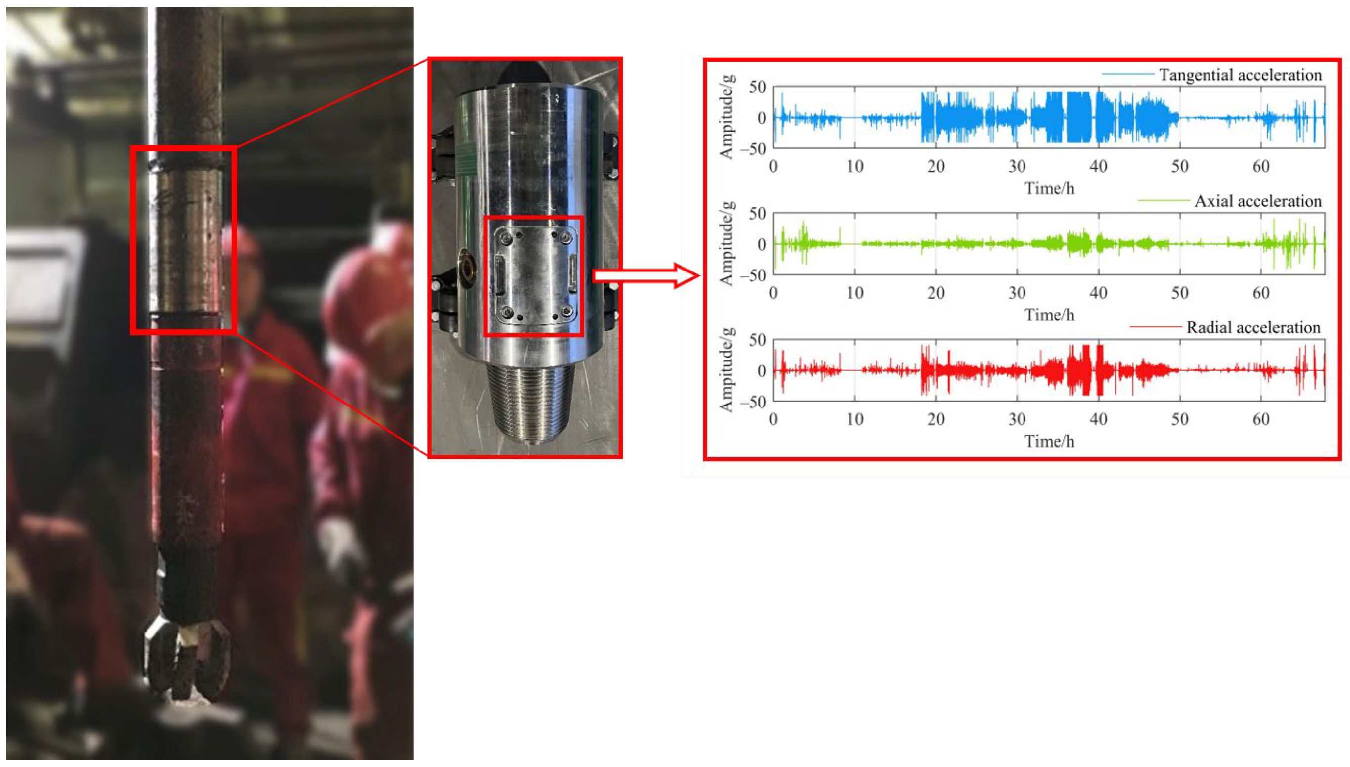
3.1. Source of Downhole Measured Datasets

The analytical experiments in this study were based on drilling datasets from 5449 to 5635 m. These data come from the vertical section of a well in the Fuman block of Tarim Oilfield, China. The lithology is Carboniferous and Devonian. Figure 3 and Figure 4 show that the near-bit measurement tool consists of the following parameters: φ215.9 mm PDC bit + φ172 mm torque impactor + φ178 mm near-bit measurement sub. It is worth noting that these data were obtained through near-bit measurement. During the field test, the near-bit measurement sub operated continuously for 30 h with a sampling frequency of 400 Hz. The near-bit measurement sub is equipped with a triaxial accelerometer, gyroscope, temperature sensor, etc. It can measure and continuously store time series data of downhole three-axis vibration (±40 g, g is gravity acceleration), rotation per minute (±333 r/min), weight on bit (±300 kN), torque (±30 kN·M), temperature (150 °C), etc. Therefore, the data obtained from the near-bit measurement sub can be used to approximate the working state of the bit and further analyze the downhole conditions. Here, the triaxial accelerometer is eccentrically mounted, and the measurement equation is as follows:

$$\left\{\begin{array}{l}X=a_x+r{\displaystyle \frac{\mathrm{d}\omega }{dt}}\\ Y=a_y+r{\omega }^2\\ Z=a_z\end{array}\right.$$

(25)

The measured X, Y, and Z are the tangential, radial, and axial accelerations, respectively. $a_x$ and $a_y$ are the lateral acceleration components of the drill string near the drill bit, $a_z$ is the axial acceleration component, r is the eccentric distance, and $\omega$ is the angular velocity.

Figure 3. Near-bit measuring tool.

Figure 3. Near-bit measuring tool.

Figure 4. Field application diagram of near-bit measuring tool.

Figure 4. Field application diagram of near-bit measuring tool.

In particular, four types of data—normal drilling, stick–slip, HFTO, and HFTO coupled with stick–slip vibration—are selected from the field data for comparison. Furthermore, time-domain and frequency-domain analysis techniques are used to process the data for a more intuitive observation of the characteristics of HFTO.

Figure 5 shows the triaxial vibration data measured on the field. During phase t1, the drilling is normal and there is no periodic fluctuation in the triaxial acceleration. Additionally, the triaxial acceleration’s amplitude is relatively small. During phase t2, compared to normal drilling, the amplitudes of triaxial vibration acceleration show a synchronous increase. Notably, the increase in tangential acceleration amplitude is particularly pronounced, exceeding 40 g. Existing research has suggested that high tangential acceleration amplitudes indicate HFTO occurring downhole. Additionally, the limited bandwidth of the triaxial accelerometers results in a flat-topped waveform in the tangential acceleration amplitude, which means that the actual downhole HFTO may be more severe than measured.

Figure 6 shows the triaxial vibration data during stick–slip vibration. The stick–slip vibration exhibits an apparent periodic fluctuation with approximately 9 s. The stick phase is kept for 3 s, as shown in t1, and the slip phase is kept for 6 s, as shown in t2.

Figure 7 shows the triaxial vibration data during HFTO coupled with stick–slip vibration. It is clear that the stick and slip phases are still present. The vibration amplitudes in different directions increase significantly during the slip phase. It can be highlighted that the tangential acceleration amplitude is much higher than that of only stick–slip vibration due to the torque generated by the bit–rock interaction being regarded as an external excitation source for HFTO. During the stick phase, this force temporarily disappears, resulting in a rapid decrease in tangential acceleration.

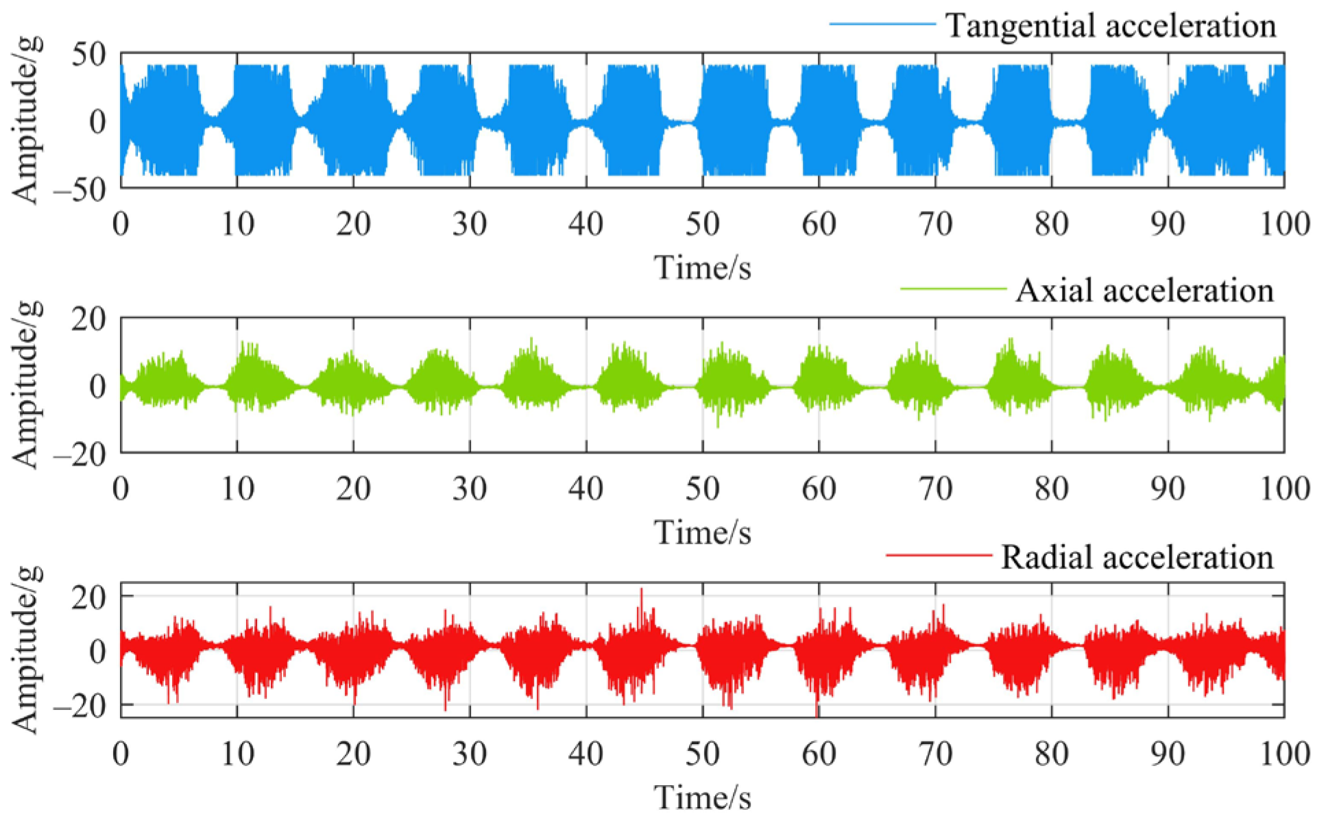
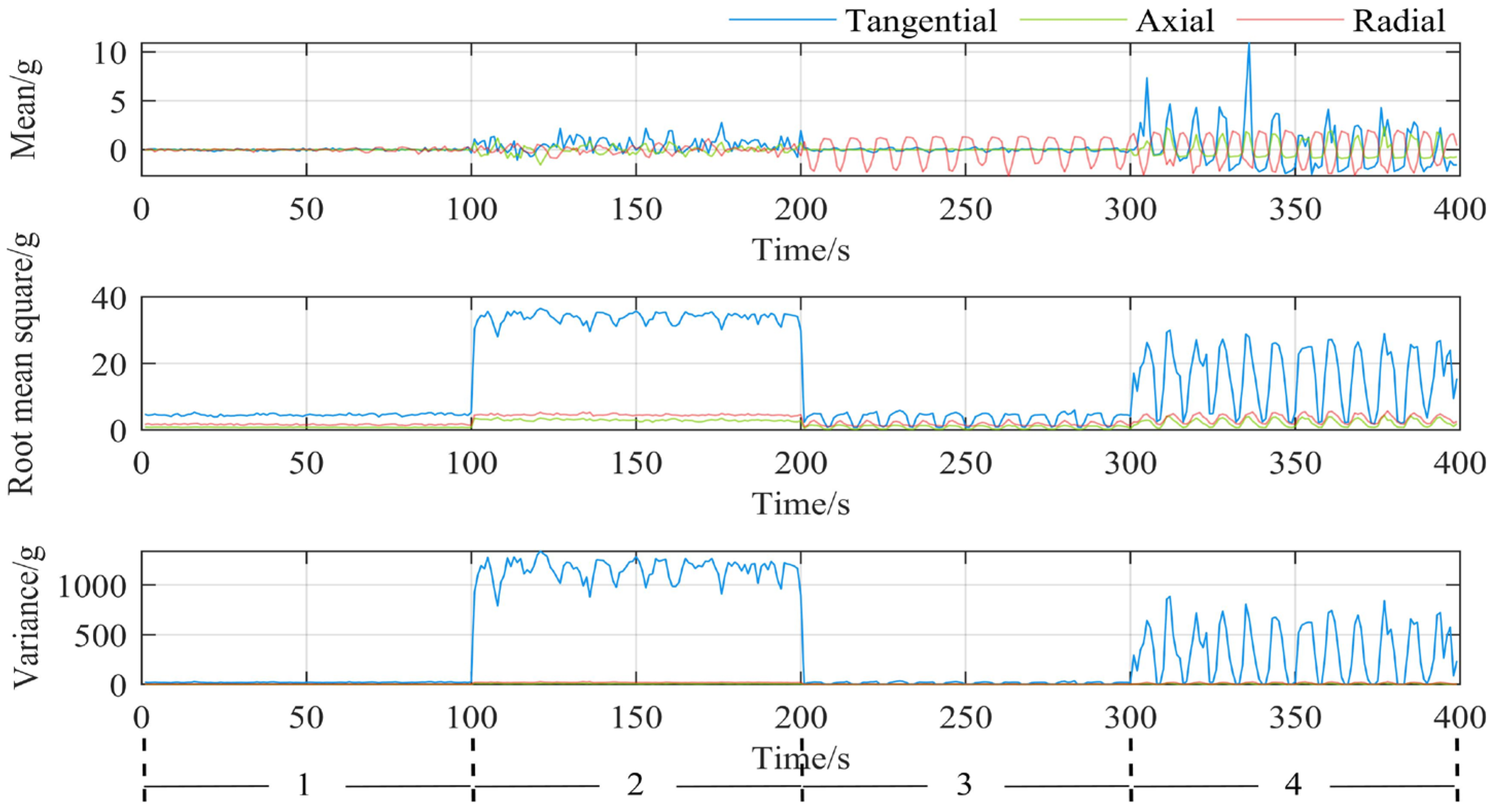
3.2. Time Domain Analysis

Figure 8 depicts the curves for the mean, variance, and root mean square (RMS) of triaxial acceleration. Region 1 represents normal drilling data, region 2 represents HFTO data, region 3 represents stick–slip vibration data, and region 4 represents data where HFTO is coupled with stick–slip vibration. It can be observed that when HFTO occurs, the RMS value and variance of the tangential acceleration are elevated, indicating that tangential acceleration more accurately captures the characteristics of HFTO. Compared to regions 2 and 3, region 4 shows that the trend observed in the curve follows the behavior of stick–slip and HFTO. On the one hand, the curves show periodic fluctuations; on the other hand, the RMS value and variance of tangential acceleration are significantly higher than stick–slip alone. Notably, the mean value of the tangential acceleration is greater than that of the radial acceleration during coupling vibrations, which is opposite to stick–slip. Therefore, the result can serve as a distinguishing criterion from stick–slip vibration.

3.3. Time Frequency Domain Analysis

Figure 9 shows the time-frequency diagrams for three conditions: stick–slip, HFTO, and the coupling of HFTO with stick–slip. Figure 9a displays a dominant frequency of 0.128 Hz in the spectrum of the radial acceleration, which is consistent with the characteristics of energy concentration at low frequencies during stick–slip occurrence. Therefore, the enhancement of low-frequency components in the radial vibration spectrum can be considered an essential characteristic of stick–slip. As shown in Figure 9b, when HFTO occurs, the tangential and radial vibration spectrum exhibits a dominant frequency of 177 Hz during HFTO, which then shifts to 61 Hz. This phenomenon is related to the changes in WOB observed in field data. Additionally, the tangential acceleration’s amplitude in the spectrum is noticeably larger than the radial acceleration’s. Figure 9c shows that when HFTO is coupled with stick–slip vibration, the tangential acceleration exhibits a dominant frequency of 61 Hz. Notably, the radial acceleration displays dominant frequencies of 61 Hz and 0.128 Hz. This means that the coupled vibration spectrum contains dominant frequencies of both HFTO and stick–slip.

4. Experimentation and Analysis

4.1. Improved Whale Algorithm Performance Test

The TSWOA’s performance is validated via a comparative experiment with the WOA. Each of the four benchmark test functions in

Table 1. Test function information table.

Number	Function Name	Dimension	Search Space
F1	Schwefel 2.22	30	[−100,100]
F2	Quartic Function	30	[−1.28,1.28]
F3	Ackley’s Function	30	[−32,32]
F4	Penalized Function	30	[−50,50]

is run independently 30 times, with the mean and standard deviation as test metrics. Finally, the images of the optimization process of the functions and test results are obtained. Among them, the relevant parameters included population size of 30 and maximum iterations of 1000.

Figure 10 shows the 3D images of the four benchmark test functions and the convergence curves of the algorithms. The colors in the 3D image are typically associated with the Z-axis coordinate value. As the Z-axis values gradually increase, the colors transition from blue and green to yellow and orange. For Function F1, the convergence speed of TSWOA is significantly faster than that of WOA, indicating superior performance. For functions F2 to F4, TSWOA reaches the optimal value first, demonstrating that its optimization accuracy, speed, and global search capability are all superior to those of WOA.

The outcomes of the benchmark function testing are shown in

Table 2. Benchmark function test results.

Test Function	Algorithm	Average Value	Standard Deviation
Schwefel 2.22	WOA	1.00 × 10−106	3.69 × 10−122
	TSWOA	0	0
Quartic Function	WOA	5.96 × 10−3	8.82 × 10−19
	TSWOA	9.87 × 10−7	4.31 × 10−22
Ackley’s Function	WOA	7.99 × 10−15	0
	TSWOA	8.88 × 10−16	0
Penalized Function	WOA	1.16 × 10−3	8.82 × 10−19
	TSWOA	2.56 × 10−24	3.74 × 10−40

. For Function F1, from the mean and standard deviation, it can be seen that TSWOA always finds the theoretical extreme value of 0, while WOA can only find a value approaching 0. The result shows that the TSWOA exhibits better stability and optimization performance. For functions F2 to F4, both the mean and standard deviations of TSWOA are more minor than those of WOA, indicating superior optimization accuracy and stronger global search optimization power for the TSWOA.

4.2. Experiment for Identifying HFTO

4.2.1. Data Preprocessing

The selected experimental data include four conditions: stick–slip, HFTO, normal drilling, and the coupling of HFTO with stick–slip. In this study, numbers 1, 2, 3, and 4 are, respectively, used to represent the four conditions as data labels. The numbering of data labels and the distribution of the dataset are shown in

Table 3. Distribution of data label numbers and datasets.

Working Condition	Labels	Sample Size of the Dataset (Group)
Stick–slip	1	300
HFTO	2	300
Normal drilling	3	300
Coupled vibration	4	300

. Due to factors such as the complex downhole environment and errors inherent in sensors, high-frequency vibration data often contain noise, which can affect the training results of the model. Therefore, a three-level wavelet decomposition method is used to denoise the raw data before feature extraction, and the denoised signal is reconstructed using the wavelet function db3.

As shown in Figure 6, the stick–slip vibration exhibits periodic oscillations for 9 s. Therefore, a data segment is selected every 10 s to ensure that each segment contains at least one complete cycle of the stick and slip phases. Ultimately, each operating condition includes 300 sets of data, with each set including RPM, torque, and triaxial vibration.

The triaxial vibration data are analyzed in the time domain, yielding eight time-domain features: mean, standard deviation, root mean square, kurtosis, skewness, waveform factor, pulse factor, and kurtosis factor. Fast Fourier Transform is applied to each set of data to obtain five frequency-domain features for rotational speed, torque, and triaxial vi-bration, including mean amplitude, centroid frequency, frequency variance, root mean square frequency, and frequency standard deviation. In total, 25 time-domain features and 24 frequency-domain features are obtained.

For the problem of high dimensionality in the 49-dimensional data and the presence of certain correlations between features, the principal component analysis (PCA) is used in this study to create new composite variables and decrease the dimensionality of the feature data [45,46]. The method of calculating the cumulative percent variance (CPV) is as follows:

$$CP{V}_{\mathrm{k}}={\displaystyle \sum _{i=1}^{k}P{V}_i={\displaystyle \sum _{i=1}^k\left(\frac{{\lambda }_i}{{\displaystyle \sum _{j=1}^m{\lambda }_j}}\right)}}$$

(26)

where $P{V}_i$ is the contribution rate of the variance, $P{V}_i={\displaystyle \frac{{\lambda }_i}{{\displaystyle \sum _{j=1}^m{\lambda }_j}}}$.

The 49 eigenvalues are used as input variables; the variance is explained and the cumulative variance interpretation rate for these variables is calculated in Figure 11.

Figure 11 shows that when the feature dimension of vibration signal after dimensionality reduction is 9, the cumulative explanatory variance contribution rate reaches over 95%, and after which the contribution rate curve begins to stabilize. This indicates that using the first nine principal components in this study can achieve effective classification and recognition of HFTO.

4.2.2. TSWOA-SVM Downhole Drilling Conditions Recognition Model

To validate the superiority of the established TSWOA-SVM model in identifying HFTO, three other algorithmic models—GA-SVM, GWO-SVM, and WOA-SVM—are considered for comparison. The models are built using the same training set and tested for their ability to recognize HFTO using a test set. The flowchart for identifying downhole drill string vibration patterns (including HFTO) using the TSWOA-SVM model is shown in Figure 12. The next section will introduce and discuss in detail the results of performance comparison among all models.

4.2.3. Analysis of Results

This study uses accuracy, recall, precision, and F1 score as performance indicators to evaluate the classification identification results of the algorithm model for downhole drilling column vibration patterns (including HFTO). In comparison to other models, the corresponding model performs better in terms of prediction the higher the value of the aforementioned index. Their calculation methods are as follows:

$$Accuracy=(TP+TN)/N$$

(27)

$$Precision=TP/(TP+FP)$$

(28)

$$Recall=TP/(TP+FN)$$

(29)

$$F1={\displaystyle \frac{2\ast Precision\ast Recall}{Precision+Recall}}$$

(30)

The variables in the above indicators are based on a confusion matrix. When using a classification model to identify the categories of test data, there are four possible outcomes (assuming the two categories are True and False), defined as follows.

True Positive (TP): The classifier identifies as True, and it is actually True; False Positive (FP): The classifier identifies as True, but it is actually False; True Negative (TN): The classifier identifies as False, and it is actually False; False Negative (FN): The classifier identifies as False, but it is actually True.

The TSWOA-SVM algorithm model’s evaluation results are shown in

Table 4. Evaluation metrics for the TSWOA-SVM model.

Confusion Matrix					Precision	Recall	F1 Score
True Label	Prediction Label
	Stick–Slip	HFTO	Normal Drilling	Coupled Vibration
Stick–slip	87	1	2	0	0.989	0.967	0.978
HFTO	0	89	1	0	0.989	0.989	0.989
Normal drilling	1	0	89	0	0.937	0.989	0.962
Coupled vibration	0	0	3	87	1.000	0.967	0.983

. The TSWOA-SVM algorithm model has a precision of more than 93%, and the recall rate and F1-score are both overall above 96%.

To better demonstrate the TSWOA-SVM algorithm model’s effectiveness and superiority in the classification and detection of HFTO, other algorithm models are used to identify downhole drilling column vibration patterns (including HFTO) for comparison. GA-SVM, GWO-SVM, and WOA-SVM algorithm models are trained and tested using the same dataset. The consistency between the predicted classification of the test set by the comparative algorithm model and the actual classification of the test set is regarded as a way for evaluating the accuracy of the model prediction. Therefore, the comparison graphs of the predicted test set types and the actual types by TSWOA-, WOA-, GWO-, and GA-optimized SVM models are, respectively, plotted, as shown in Figure 13. According to the test results shown in the figures, the classification accuracies of the four classification models are 97.8% (352/360), 96.1% (346/360), 95.8% (345/360), and 92.8% (334/360), respectively. Obviously, the TSWOA-SVM model’s classification performance is significantly better than the latter three, and the classification accuracy is improved by 1.7% compared to WOA-SVM model. The aforementioned findings show that the TSWOA-SVM model has a high accuracy and can effectively identify downhole HFTO.

Additionally,

Table 5. Model evaluation comparison.

Model	Model Evaluation Indicators
	Precision/%	Recall/%	F1-Score	Accuracy/%
GA-SVM	92.778	92.778	0.928	92.778
GWO-SVM	95.958	95.833	0.958	95.833
WOA-SVM	96.235	96.111	0.961	96.111
TSWOA-SVM	97.859	97.778	0.978	97.778

also shows that the TSWOA-SVM model outperforms other algorithms mentioned above in terms of accuracy, precision, recall, and F1 score on the test set. This means that the model performs better. As a result, TSWOA proves to be a more fitting choice for the parameter optimization of the SVM applied to HFTO recognition.

Furthermore, to assess the algorithm’s generalization ability, a 5-fold cross-validation method is employed [34]. The specific steps involve randomly shuffling the original dataset and dividing it into five equal-sized subsets. One subset is used as the test set and the remaining four subsets are used as the training set, repeating the process five times. The accuracy of each iteration is calculated and the average as the result of cross-validation is taken. Figure 14 shows the 5-fold cross-validation’s average accuracy and accuracy variance. The average cross-validation accuracy of the TSWOA-SVM algorithm is 96.75%, which is an improvement of 1.67%, 3.33%, and 7.5% over the WOA-SVM, GWO-SVM, and GA-SVM algorithms, respectively. In addition, the accuracy variance of TSWOA-SVM is also the smallest. This means that the TSWOA-SVM model has a strong generalization ability and provides more accurate and stable classification results compared to other algorithms. In summary, the proposed TSWOA-SVM model demonstrates superior performance in the identification of HFTO.

5. Conclusions

(1)

An improved whale algorithm (TSWOA) is presented in this research. The innovations of the TSWOA compared to the traditional WOA lies in its utilization of the Fuch chaotic mapping with a reverse learning strategy to enhance population quality; furthermore, it introduces a simulated annealing strategy and hyperbolic tangent function to improve the algorithm’s ability to search globally. The benchmark function test results show that the TSWOA has a faster rate of convergence and effectively avoids local optima.

(2)

Using the downhole near-bit engineering parameter measurement tool to collect downhole engineering data, 400 sets of data were selected for each of the four states downhole. Each sample includes parameters such as RPM, torque, and three-axis vibration. These data provide support for the analysis and identification of downhole HFTO. The TSWOA is used for parameter optimization in SVM, and a TSWOA-SVM algorithm model is established for HFTO recognition. The TSWOA-SVM algorithm model’s classification performance is compared to that of GA-SVM, GWO-SVM, and WOA-SVM algorithm models. It is found that the TSWOA-SVM algorithm model overall outperformed the other algorithms significantly, with an accuracy of 97.8%. Therefore, TSWOA-SVM has good application prospects in high-frequency torsional vibration recognition.

(3)

To further validate the effectiveness and stability of the TSWOA-SVM, we conducted a 5-fold cross-validation experiment comparing this algorithm with GA-SVM, GWO-SVM, and WOA-SVM. The experimental results show that the TSWOA-SVM algorithm achieves a higher average cross-validation accuracy compared to the other three algorithms and has the smallest accuracy variance. This indicates that TSWOA-SVM performs more stably on different subsets of data. Therefore, TSWOA-SVM has better generalization ability and robustness.

(4)

The primary limitation of this study lies in its reliance on downhole data for feature extraction. Future research should prioritize effective extraction of latent features from both surface low-frequency data and downhole high-frequency data, thereby comprehensively integrating relationships between these datasets. Furthermore, subsequent investigations should consider incorporating transfer learning methodologies alongside the proposed TSWOA-SVM model. This approach would enhance applicability to the fused dataset and allow for the adjustment of model parameters to better accommodate characteristics of the new data. Employing test data for rigorous model validation and performance evaluation will be crucial to ensuring the stability and generalizability of the model. Ultimately, the objective is to leverage subtle variations in surface data to accurately identify HFTO.

References

1. Cai, M.; Mao, L.; Xing, X.; Zhang, H.; Li, J. Analysis on the nonlinear lateral vibration of drillstring in curved wells with beam finite element. Commun. Nonlinear Sci. Numer. Simul. 2022, 104, 106065. [Google Scholar] [CrossRef]
2. Rajabali, F.; Moradi, H.; Vossoughi, G. Coupling analysis and control of axial and torsional vibrations in a horizontal drill string. J. Petrol. Sci. Eng. 2020, 195, 107534. [Google Scholar] [CrossRef]
3. Caballero, E.F.; Lobo, D.M.; Di Vaio, M.V.; Silva, E.; Ritto, T.G. Support vector machines applied to torsional vibration severity in drill strings. J. Braz. Soc. Mech. Sci. Eng. 2021, 43, 386. [Google Scholar] [CrossRef]
4. Shen, Y.; Zhang, Z.; Zhao, J.; Chen, W.; Hamzah, M.; Harmer, R.; Downton, G. The Origin and Mechanism of Severe Stick-Slip. In Proceedings of the SPE Annual Technical Conference and Exhibition, San Antonio, TX, USA, 9–11 October 2017. [Google Scholar] [CrossRef]
5. Nordin, M.H.; Looi, L.K.; Slagel, P.; Othman, M.H.; Affandi, A.R.; Zurhan, M.S. Minimising Torsional Vibration Due to Stick Slip Using Z Technology for Drilling Energy Efficiency in Multiple Hard Stringers Field in Offshore Malaysia. In Proceedings of the International Petroleum Technology Conference, Virtual, 23 March–1 April 2021. [Google Scholar] [CrossRef]
6. Hu, J.; Guo, Q.; Sun, Z.; Yang, D. Study on low-frequency torsional vibration suppression of integrated electric drive system considering nonlinear factors. Energy 2023, 284, 129251. [Google Scholar] [CrossRef]
7. Sharma, A.; Abid, K.; Srivastava, S. A review of torsional vibration mitigation techniques using active control and machine learning strategies. Petroleum 2024, 10, 411–426. [Google Scholar] [CrossRef]
8. Jain, J.R.; Oueslati, H.; Hohl, A.; Reckmann, H.; Ledgerwood, L.W.; Tergeist, M.; Ostermeyer, G.P. High-frequency torsional dynamics of drilling systems: An analysis of the bit-system interaction. In Proceedings of the IADC/SPE Drilling Conference and Exhibition, Fort Worth, TX, USA, 4–6 March 2014. [Google Scholar] [CrossRef]
9. Eli, E.; Armin, K.; Xu, H.; Sui-Long, L.; Dennis, H.; Hanno, R.; John, B. Testing and Characterization of High-Frequency Torsional Oscillations in a Research Lab to Develop New HFTO Suppressing Solutions. In Proceedings of the SPE/IADC International Drilling Conference and Exhibition, Stavanger, Norway, 7–9 March 2023. [Google Scholar] [CrossRef]
10. Zhang, Y.; Zhang, H.; Chen, D.; Ashok, P.; van Oort, E. Comprehensive review of high frequency torsional oscillations (HFTOs) while drilling. J. Pet. Sci. Eng. 2023, 220, 111161. [Google Scholar] [CrossRef]
11. Lines, L.A.; Stroud, D.R.; Coveney, V.A. Torsional resonance—An understanding based on field and laboratory tests with latest generation point-the-bit rotary steerable system. In Proceedings of the SPE/IADC Drilling Conference, Amsterdam, The Netherlands, 5–7 March 2013. [Google Scholar] [CrossRef]
12. Zhang, Z.; Shen, Y.; Chen, W.; Shi, J.; Bonstaff, W.; Tang, K.; Smith, D.L.; Arevalo, Y.I.; Jeffryes, B. Continuous high frequency measurement improves understanding of high frequency torsional oscillation in North America land drilling. In Proceedings of the SPE Annual Technical Conference and Exhibition, San Antonio, TX, USA, 9–11 October 2017. [Google Scholar] [CrossRef]
13. Shen, Y.; Chen, W.; Zhang, Z.; Bowler, A.; Jeffryes, B.; Chen, Z.; Carrasquilla, M.N.; Smith, D.; Skoff, G.; Panayirci, H.M.; et al. Drilling dynamics model to mitigate high frequency torsional oscillation. In Proceedings of the IADC/SPE International Drilling Conference and Exhibition, Galveston, TX, USA, 3–5 March 2020. [Google Scholar] [CrossRef]
14. Xie, X.; Zhang, T.; Lin, Z.; Xu, C.; Li, Y.; Guo, H. Analysis on downhole high-frequency torsional oscillation of bottom hole assembly. China Pet. Mach. 2022, 50, 79–84. [Google Scholar] [CrossRef]
15. Kulke, V.; Thunich, P.; Schiefer, F.; Ostermeyer, G.P. A method for the design and optimization of nonlinear tuned damping concepts to mitigate self-excited drill string vibrations using multiple scales lindstedt-poincaré. Appl. Sci. 2021, 11, 1559. [Google Scholar] [CrossRef]
16. Kulke, V.; Ostermeyer, G.P. Energy transfer through parametric excitation to reduce self-excited drill string vibrations. J. Vib. Control 2022, 28, 3344–3351. [Google Scholar] [CrossRef]
17. de Souza, R.L.B.; Fadhel, H.A.; Malik, K.A. Drilling Optimization using High Frequency Data Measuring Torsional Oscillations (HFTO) and Corresponding Frequencies Provided by Downhole Tools, Supported by Extensive Scientific Pre-Job BHA Modeling Allows to Reduce Downhole Tool Failures and Improve Performance. In Proceedings of the International Petroleum Technology Conference, Dhahran, Saudi Arabia, 12 February 2024. [Google Scholar] [CrossRef]
18. Hohl, A.; Tergeist, M.; Oueslati, H.; Herbig, C.; Ichaoui, M.; Ostermeyer, G.P.; Reckmann, H. Prediction and mitigation of torsional vibrations in drilling systems. In Proceedings of the IADC/SPE Drilling Conference and Exhibition, Fort Worth, TX, USA, 1–3 March 2016. [Google Scholar] [CrossRef]
19. Sugiura, J.; Jones, S. Simulation and measurement of high-frequency torsional oscillation (HFTO)/High-frequency axial oscillation (HFAO) and downhole HFTO mitigation: Knowledge gains continue using embedded high-frequency drilling dynamics sensors. SPE Drill. Complet. 2020, 35, 553–575. [Google Scholar] [CrossRef]
20. Ichaoui, M.; Ostermeyer, G.P.; Tergeist, M.; Hohl, A. Estimation of high-frequency vibration loads in deep drilling systems using augmented Kalman filters. In Proceedings of the ASME 2020 International Mechanical Engineering Congress and Exposition, Virtual, 16–19 November 2020. [Google Scholar] [CrossRef]
21. Hohl, A.; MacFarlane, D.; Larsen, D.S.; Olsnes, K.; Grymalyuk, S.; Gatzen, M.; Hovda, S. Utilizing downhole sampled high-frequency torsional oscillation measurements for identifying stringers and minimizing operational invisible lost time ILT. In Proceedings of the SPE Annual Technical Conference and Exhibition, Dubai, United Arab Emirates, 21–23 September 2021. [Google Scholar] [CrossRef]
22. Sugiura, J.; Jones, S. A drill bit and a drilling motor with embedded high-frequency (1600 Hz) drilling dynamics sensors provide new insights into challenging downhole drilling conditions. SPE Drill. Complet. 2019, 34, 223–247. [Google Scholar] [CrossRef]
23. Hohl, A.; Kulke, V.; Ostermeyer, G.P.; Kueck, A.; Peters, V.; Reckmann, H. Design and field deployment of a torsional vibration damper. In Proceedings of the IADC/SPE International Drilling Conference and Exhibition, Galveston, TX, USA, 8–10 March 2022. [Google Scholar] [CrossRef]
24. Kueck, A.; Hohl, A.; Schepelmann, C.; Lam, S.-L.; Heinisch, D.; Herbig, C.; Kulke, V.; Ostermeyer, G.-P.; Reckmann, H.; Peters, V. Break-through in elimination of high-frequency torsional oscillations through new damping tool proven by field testing in the US. In Proceedings of the Offshore Technology Conference, Houston, TX, USA, 2–5 May 2022. [Google Scholar] [CrossRef]
25. Hanafy, A.; Kueck, A.; Pauli, A.; Huang, X.; Bomidi, J. The Benefit of In-Bit Sensing For Efficient Drilling of Deep Reach Lateral Wells in HFTO Prone Interbedded Abrasive Lithologies in North America Land. In Proceedings of the International Petroleum Technology Conference, Dhahran, Saudi Arabia, 12–13 February 2024. [Google Scholar] [CrossRef]
26. Millan, E.; Ringer, M.; Boualleg, R.; Li, D. Real-time Drillstring Vibration Characterization Using Machine Learning. In Proceedings of the SPE/IADC International Drilling Conference and Exhibition, The Hague, The Netherlands, 5–7 March 2019. [Google Scholar] [CrossRef]
27. Hegde, C.; Millwater, H.; Gray, K. Classification of drilling stick slip severity using machine learning. J. Pet. Sci. Eng. 2019, 179, 1023–1036. [Google Scholar] [CrossRef]
28. Gupta, S.; Chatar, C.; Celaya, J.R. Machine learning lessons learnt in stick-slip prediction. In Proceedings of the Abu Dhabi International Petroleum Exhibition & Conference, Abu Dhabi, United Arab Emirates, 11–14 November 2019. [Google Scholar] [CrossRef]
29. Naraghi, M.; Ezzatyar, P.; Jamshidi, S. Prediction of drilling pipe sticking by active learning method (ALM). J. Pet. Gas Eng. 2013, 4, 173–183. [Google Scholar] [CrossRef]
30. Chamkalani, A.; Pordel Shahri, M.; Poordad, S. Support vector machine model: A new methodology for stuck pipe prediction. In Proceedings of the SPE Unconventional Gas Conference and Exhibition, Muscat, Oman, 28–30 January 2013. [Google Scholar] [CrossRef]
31. Fu, H.; Zhang, T.; Li, Y.; Liu, Y. Research on PCA-SVM stuck prediction based on downhole parameters. Comput. Simul. 2021, 38, 386–390. [Google Scholar]
32. Hohl, A.; Kulke, V.; Kueck, A.; Herbig, C.; Reckmann, H.; Ostermeyer, G.P. The Nature of the Interaction Between Stick/Slip and High-Frequency Torsional Oscillations. In Proceedings of the IADC/SPE International Drilling Conference and Exhibition, Galveston, TX, USA, 3–5 March 2020. [Google Scholar] [CrossRef]
33. Oueslati, H.; Jain, J.R.; Reckmann, H.; Ledgerwood, L.W.; Pessier, R.; Chandrasekaran, S. New insights into drilling dynamics through high-frequency vibration measurement and modeling. In Proceedings of the SPE Annual Technical Conference and Exhibition, New Orleans, LA, USA, 30 September–2 October 2013. [Google Scholar] [CrossRef]
34. Chen, X.; Zhang, S.; Yang, P. Prediction on hot rolled strip width based on improved BOA-ELM. Forg. Stamp. Technol. 2024, 49, 101–106+126. [Google Scholar]
35. Li, C.; Mi, X.; Cui, X. Optimization of cold chain logistics distribution routing based on improved ant colony algorithm with hyperbolic tangent function. J. Highw. Transp. Res. Dev. 2023, 40, 236–244+258. [Google Scholar]
36. Huang, Y.; Yuan, B.; Xu, S. Fault diagnosis of permanent magnet synchronous motor of coal mine belt conveyor based on digital twin and ISSA-RF. Processes 2022, 10, 1679. [Google Scholar] [CrossRef]
37. Zhang, J.; Wang, L. Fault diagnosis of hydraulic pumps based on support vector machine optimized by beetle antennae search. Noise Vib. Control 2022, 42, 105–109. [Google Scholar]
38. Eskandari, A.; Milimonfared, J.; Aghaei, M. Autonomous monitoring of line-to-line faults in photovoltaic systems by feature selection and parameter optimization of support vector machine using genetic algorithms. Appl. Sci. 2020, 10, 5527. [Google Scholar] [CrossRef]
39. Li, C.; Zhou, J.; Du, K.; Dias, D. Stability prediction of hard rock pillar using support vector machine optimized by three metaheuristic algorithms. Int. J. Min. Sci. Technol. 2023, 33, 1019–1036. [Google Scholar] [CrossRef]
40. Rana, N.; Latiff, M.S.A.; Abdulhamid, S.M.; Chiroma, H. Whale optimization algorithm: A systematic review of contemporary applications, modifications and developments. Neural Comput. Appl. 2020, 32, 16245–16277. [Google Scholar] [CrossRef]
41. Uzer, M.S.; Inan, O. Application of improved hybrid whale optimization algorithm to optimization problems. Neural Comput. Appl. 2023, 35, 12433–12451. [Google Scholar] [CrossRef]
42. Chakraborty, S.; Sharma, S.; Saha, A.K.; Saha, A. A novel improved whale optimization algorithm to solve numerical optimization and real-world applications. Artif. Intell. Rev. 2022, 55, 4605–4716. [Google Scholar] [CrossRef]
43. Nadimi-Shahraki, M.H.; Zamani, H.; Asghari Varzaneh, Z.; Mirjalili, S. A systematic review of the whale optimization algorithm. theoretical foundation, improvements, and hybridizations. Arch. Comput. Methods Eng. 2023, 30, 4113–4159. [Google Scholar] [CrossRef]
44. Shi, Q.; Zhang, H. Fault Diagnosis of an Autonomous Vehicle With an Improved SVM Algorithm Subject to Unbalanced Datasets. IEEE Trans. Ind. Electron. 2021, 68, 6248–6256. [Google Scholar] [CrossRef]
45. Pule, M.; Matsebe, O.; Samikannu, R. Application of PCA and SVM in fault detection and diagnosis of bearings with varying speed. Math. Probl. Eng. 2022, 1, 5266054. [Google Scholar] [CrossRef]
46. Kumar, A.; Gandhi, C.P.; Vashishtha, G.; Kundu, P.; Tang, H.; Glowacz, A.; Shukla, R.K.; Xiang, J. VMD based trigonometric entropy measure: A simple and effective tool for dynamic degradation monitoring of rolling element bearing. Meas. Sci. Technol. 2021, 33, 014005. [Google Scholar] [CrossRef]
Figure 2. Flow chart of TSWOA optimizing SVM.
Processes 12 02153 g002
Figure 5. Variation curve of triaxial vibration during normal drilling and HFTO.
Processes 12 02153 g005
Figure 6. Variation curve of triaxial vibration during stick–slip.
Processes 12 02153 g006
Figure 7. Variation curve of triaxial vibration during coupled vibration.
Processes 12 02153 g007
Figure 8. The curve of mean, root mean square, and variance of triaxial acceleration.
Processes 12 02153 g008
Figure 9. Time-frequency diagram.
Processes 12 02153 g009
Figure 10. Convergence curves of WOA and TSWOA under different test functions. (a) Function F1 image and convergence curve; (b) Function F2 image and convergence curve; (c) Function F3 image and convergence curve; (d) Function F4 image and convergence curve.
Processes 12 02153 g010
Figure 11. Changes in variance explained and cumulative variance interpretation rate of principal components.
Processes 12 02153 g011
Figure 12. Flowchart of HFTO recognition based on TSWOA-SVM model.
Processes 12 02153 g012
Figure 13. Classification effect of model on test set. (a) TSWOA-SVM; (b) WOA-SVM; (c) GWO-SVM; (d) GA-SVM.
Processes 12 02153 g013
Figure 14. Average accuracy and accuracy variance of 5-fold cross validation for different algorithms.
Processes 12 02153 g014