
Integrated Waterflooding Effect Evaluation Methodology for Carbonate Fractured–Vuggy Reservoirs Based on the Unascertained Measure–Mahalanobis Distance Theory

Abstract
:1. Introduction
2. Literature Review
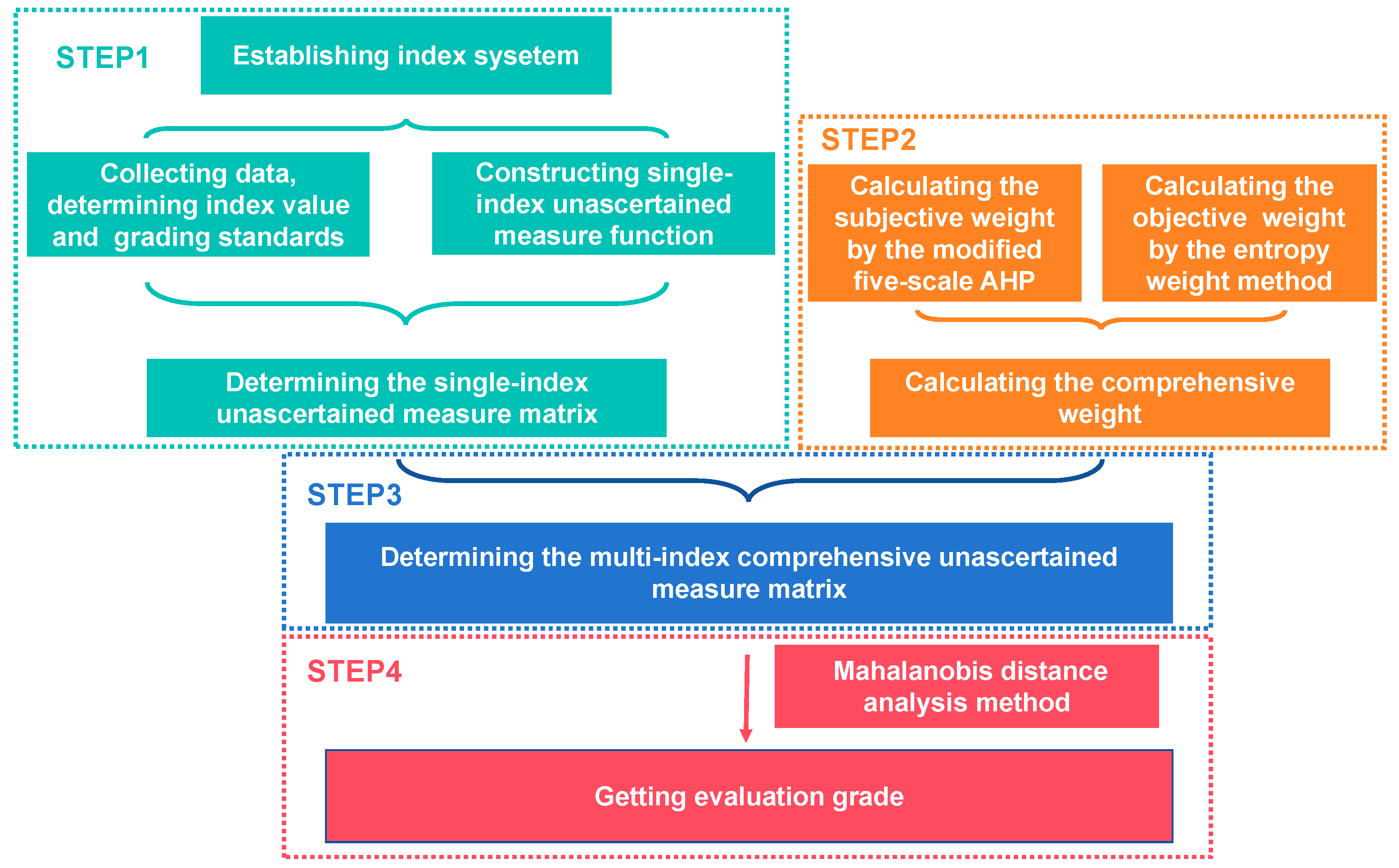
3. Model Development Procedures
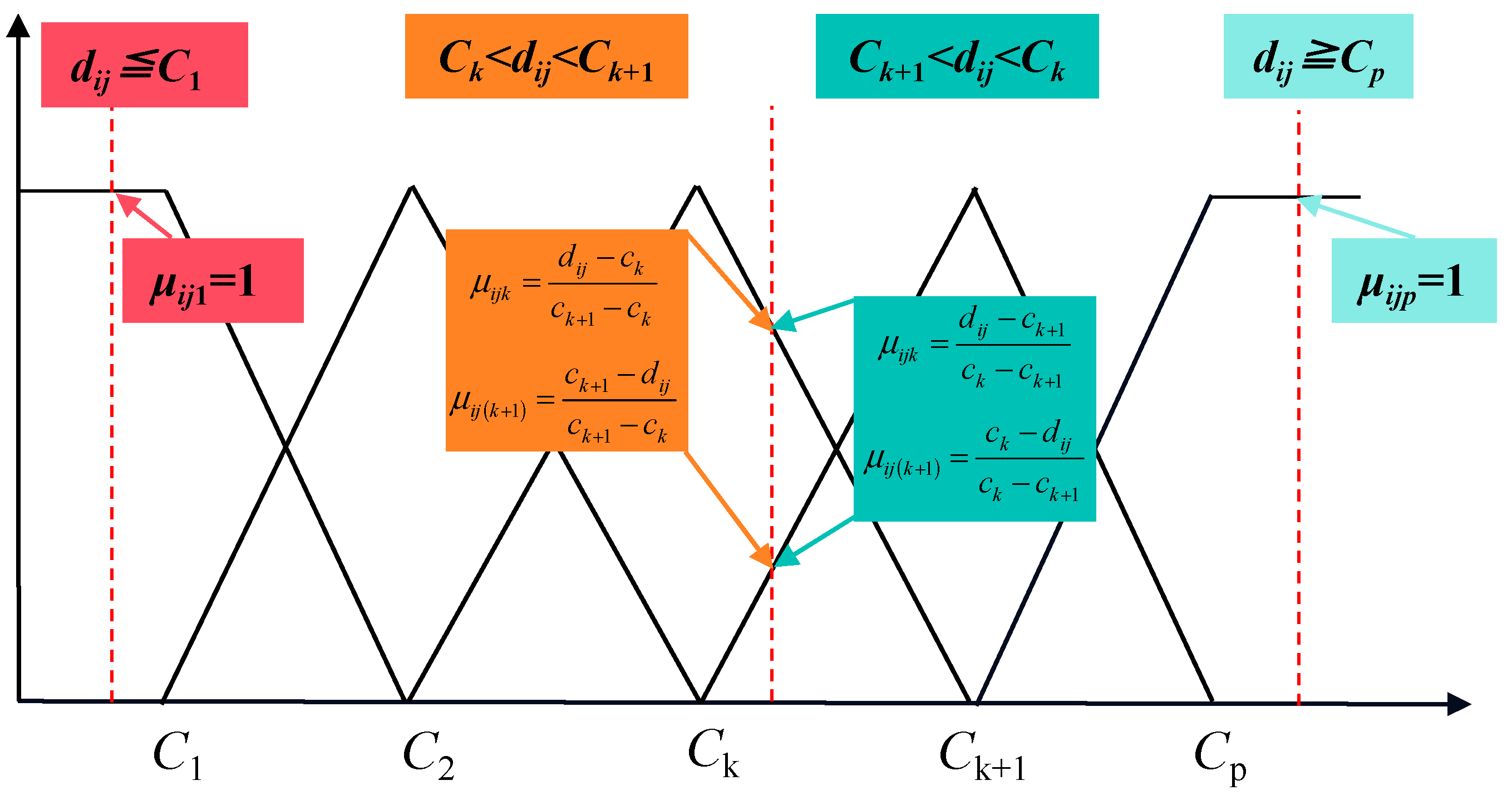
3.1. Single-Index Unascertained Measure Definition
3.2. Comprehensive Index Weight Determination
3.3. Multi-index Comprehensive Unascertained Measure Calculation
3.4. Grade Evaluation with the Mahalanobis Distance Method
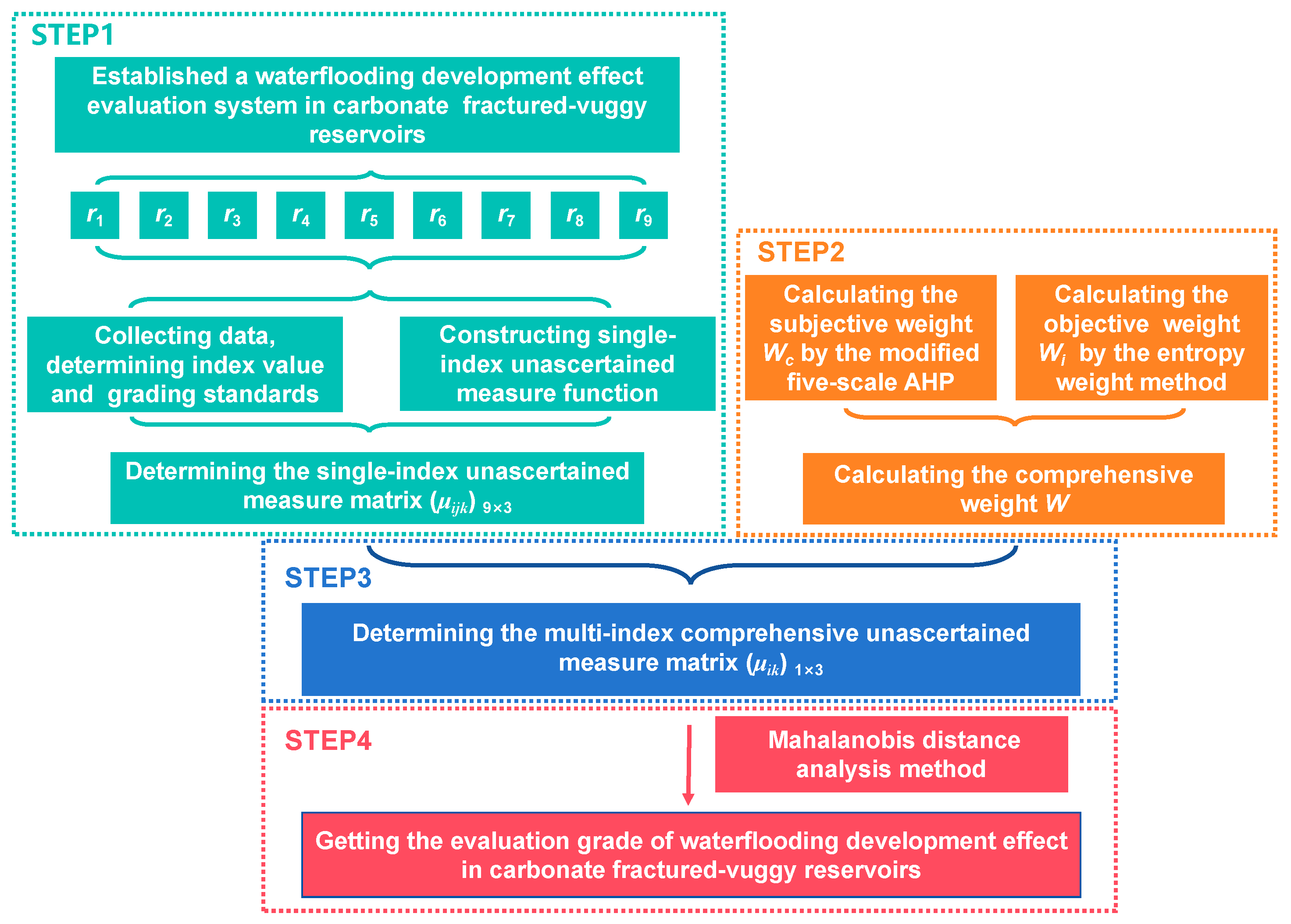
4. Waterflooding Development Effect Evaluation of the Fractured–Vuggy Carbonate Reservoir
4.1. Establishment of the Waterflooding Development Effect Evaluation System
4.2. Waterflooding Development Effect Evaluation Based on the Unascertained Measure
4.2.1. Single-Index Unascertained Measure Calculation
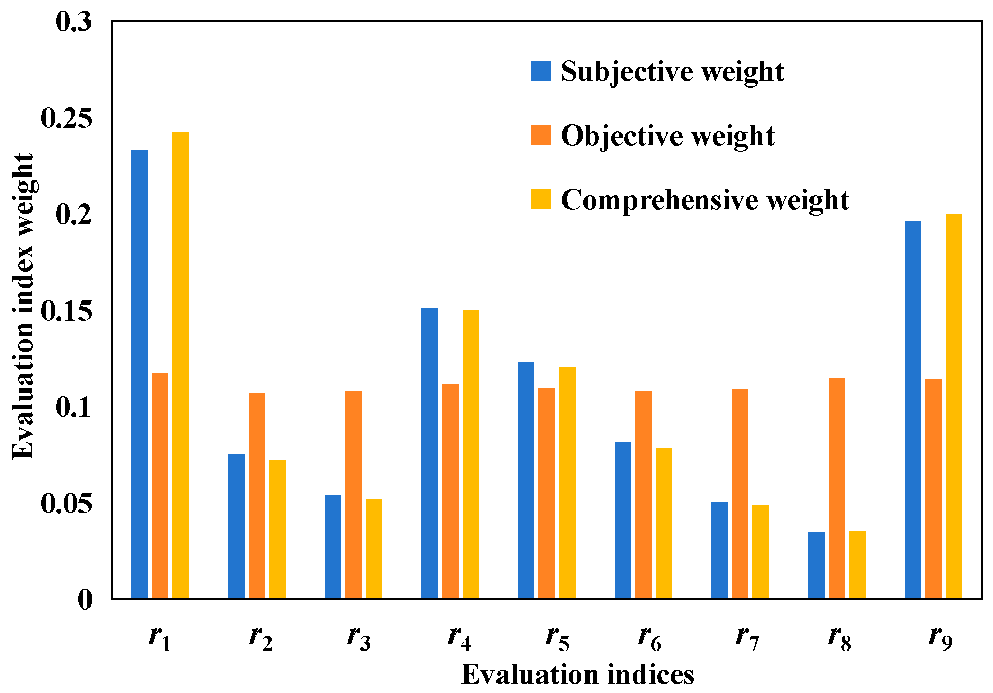
4.2.2. Comprehensive Index Weight Calculation
4.2.3. Multi-Index Comprehensive Unascertained Measure Calculation
4.2.4. Model Calculation Results with Validations
5. Conclusions
Author Contributions
Funding
Data Availability Statement
Conflicts of Interest
References
- Li, Y. The Theory and Method for Development of Carbonate Fractured-Cavity Reservoirs in T Oilfield. Acta Pet. Sin. 2013, 34, 115–121. [Google Scholar]
- Wang, D.; Sun, J. Oil Recovery for Fractured-Vuggy Carbonate Reservoirs by Cyclic Water Huff and Puff: Performance Analysis and Prediction. Sci. Rep. 2019, 9, 15231. [Google Scholar] [CrossRef]
- Li, Y.; Kang, Z.; Xue, Z.; Zheng, S. Theories and Practices of Carbonate Reservoirs Development in China. Pet. Explor. Dev. 2018, 45, 669–678. [Google Scholar] [CrossRef]
- Bois, C.; Bouche, P.; Pelet, R. Global Geologic History and Distribution of Hydrocarbon Reserves. AAPG Bull. 1982, 66, 1248–1270. [Google Scholar] [CrossRef]
- Lu, G.; Zhang, L.; Liu, Q.; Xu, Q.; Zhao, Y.; Li, X.; Deng, G.; Wang, Y. Experiment Analysis of Remaining Oil Distribution and Potential Tapping for Fractured-Vuggy Reservoir. J. Pet. Sci. Eng. 2022, 208, 109544. [Google Scholar] [CrossRef]
- Ji, B.; Zheng, S.; Gu, H. On the Development Technology of Fractured-Vuggy Carbonate Reservoirs: A Case Study on T Oilfield and Shunbei Oil and Gas Field. Oil Gas Geol. 2022, 43, 1459–1465. [Google Scholar]
- Luo, J.; Lu, X.; Wu, B.; He, X.; Li, X.; Wang, L. A Water Breakthrough Warning System of High-Yield Wells in Fractured-Vuggy Reservoirs in T Oilfield. Pet. Explor. Dev. 2013, 40, 501–506. [Google Scholar] [CrossRef]
- Guthrie, R.; Greenberger, M. The Use of Multiple Correlation Analyses for Interpreting Petroleum-Engineering Data. In Drilling and Production Practice; American Petroleum Institute: Washington, DC, USA, 1955; pp. 135–137. [Google Scholar]
- Rogers, J.B.; Terry, R.E. Applied Petroleum Reservoir Engineering, 3rd ed.; Pearson Education: Beijing, China, 2015. [Google Scholar]
- Zhang, J. Evaluation Methods of Development Effect for Water Drive Oilfield and Development Trend. Lithol. Reserv. 2012, 24, 118–122. [Google Scholar]
- Zhi, L. Using System Analysis Method to Evaluate Waterflooding Effect of Waterflooding Oilfield. In Proceedings of the International Conference on Frontier Computing, Singapore, 10–13 July 2020. [Google Scholar]
- Zhang, J.; Wang, M.; Gong, P.; Yang, Z.; Liu, X. Study on Water Injection Formula by Grey Correlation Method for Offshore Water Flooding Reservoir. J. Geosci. Environ. Prot. 2018, 6, 1–11. [Google Scholar] [CrossRef]
- Jia, H.; Li, P.; Lv, W.; Ren, J.; Cheng, C.; Zhang, R.; Zhou, Z.; Liang, Y. Application of Fuzzy Comprehensive Evaluation Method to Assess Effect of Conformance Control Treatments on Water-Injection Wells. Petroleum, 2022; in press. [Google Scholar] [CrossRef]
- Zhang, P.; Feng, G. Application of Fuzzy Comprehensive Evaluation to Evaluate the Effect of Water Flooding Development. J. Pet. Explor. Prod. Technol. 2018, 8, 1455–1463. [Google Scholar] [CrossRef]
- Chen, L.; Li, C.; Li, Z.; Shi, Y.; Wan, L.; Wang, J.; Wang, Z.; Zhao, A. Quantitative Evaluation Method for Development of Water Flooding in Reservoir, Involves Establishing Evaluation Degree of Membership Degree Matrix to Evaluate Development Effect of Water Flooding in Infiltration Complex Block Reservoir. China Patent CN107038516-A, 11 August 2017. [Google Scholar]
- Guo, M.; Jiang, S.; Li, J.; Liu, L.; Liu, M.; Peng, D.; Shi, D.; Tang, X.; Tian, T.; Zhai, L.; et al. Tracer Technology Based Offshore Reservoir Water Injection Development Result Quantitatively Evaluating Method, Involves Adding Tracers in Water Wells, and Evaluating Balanced Displacement of Waterflood Development Process. China Patent CN106285647-A, 4 January 2017. [Google Scholar]
- Makhotin, I.; Orlov, D.; Koroteev, D. Machine Learning to Rate and Predict the Efficiency of Waterflooding for Oil Production. Energies 2022, 15, 1199. [Google Scholar] [CrossRef]
- Khormali, A.; Ahmadi, S. Prediction of Barium Sulfate Precipitation in Dynamic Tube Blocking Tests and Its Inhibition for Waterflooding Application Using Response Surface Methodology. J. Pet. Explor. Prod. Technol. 2023, 13, 2267–2281. [Google Scholar] [CrossRef]
- Bruce, W.A. An Electrical Device for Analyzing Oil-Reservoir Behavior. Trans. AIME 1943, 151, 112–124. [Google Scholar] [CrossRef]
- Holanda, R.; Gildin, E.; Jensen, J.; Lake, L.; Kabir, C. A State-of-the-Art Literature Review on Capacitance Resistance Models for Reservoir Characterization and Performance Forecasting. Energies 2018, 11, 3368. [Google Scholar] [CrossRef]
- Yousef, A.; Lake, L.; Jensen, J. Analysis and Interpretation of Interwell Connectivity from Production and Injection Rate Fluctuations Using a Capacitance Model. In Proceedings of the SPE/DOE Symposium on Improved Oil Recovery, Tulsa, OK, USA, 22 April 2006. [Google Scholar]
- Yousef, A.; Gentil, P.; Jensen, J.; Lake, L. A Capacitance Model to Infer Interwell Connectivity from Production and Injection Rate Fluctuations. SPE Reserv. Eval. Eng. 2006, 9, 630–646. [Google Scholar] [CrossRef]
- Sayarpour, M.; Zuluaga, E.; Kabir, C.; Lake, L. The Use of Capacitance–Resistance Models for Rapid Estimation of Waterflood Performance and Optimization. J. Pet. Sci. Eng. 2009, 69, 227–238. [Google Scholar] [CrossRef]
- Liang, X.; Weber, D.; Edgar, T.; Lake, L.; Sayarpour, M.; Al-Yousef, A. Optimization of Oil Production Based on A Capacitance Model of Production and Injection Rates. In Proceedings of the Hydrocarbon Economics and Evaluation Symposium, Dallas, TX, USA, 1 April 2007. [Google Scholar]
- Yang, X.; Hao, Z.; Liu, K.; Tao, Z.; Shi, G. An Improved Unascertained Measure-Set Pair Analysis Model Based on Fuzzy AHP and Entropy for Landslide Susceptibility Zonation Mapping. Sustainability 2023, 15, 6205. [Google Scholar] [CrossRef]
- Zhang, G.; Wang, E.; Zhang, C.; Li, Z.; Wang, D. A Comprehensive Risk Assessment Method for Coal and Gas Outburst in Underground Coal Mines Based on Variable Weight Theory and Uncertainty Analysis. Process Saf. Environ. Prot. 2022, 167, 97–111. [Google Scholar] [CrossRef]
- Ma, L.; Zhang, J.; Xu, C.; Lai, X.; Luo, Q.; Liu, C.; Li, K. Comprehensive Evaluation of Blast Casting Results Based on Unascertained Measurement and Intuitionistic Fuzzy Set. Shock Vib. 2021, 2021, 8864618. [Google Scholar] [CrossRef]
- Sheng, K.; Lai, X.; Chen, Y.; Jiang, J.; Zhou, L. Risk Assessment of Urban Gas Pipeline Based on Different Unknown Measure Functions. Teh. Vjesn. Tech. Gaz. 2021, 28, 1605–1614. [Google Scholar] [CrossRef]
- Zhou, J.; Chen, C.; Wang, M.; Khandelwal, M. Proposing a Novel Comprehensive Evaluation Model for the Coal Burst Liability in Underground Coal Mines Considering Uncertainty Factors. Int. J. Min. Sci. Technol. 2021, 31, 799–812. [Google Scholar] [CrossRef]
- Dong, L.; Zhou, Y.; Deng, S.; Wang, M.; Sun, D. Evaluation Methods of Man-Machine-Environment System for Clean and Safe Production in Phosphorus Mines: A Case Study. J. Cent. South Univ. 2021, 28, 3856–3870. [Google Scholar] [CrossRef]
- Liu, Z.; Chen, J.; Zhao, Y.; Yang, S. A Novel Method for Predicting Rockburst Intensity Based on an Improved Unascertained Measurement and an Improved Game Theory. Mathematics 2023, 11, 1862. [Google Scholar] [CrossRef]
- Zhou, J.; Chen, C.; Khandelwal, M.; Tao, M.; Li, C. Novel Approach to Evaluate Rock Mass Fragmentation in Block Caving Using Unascertained Measurement Model and Information Entropy with Flexible Credible Identification Criterion. Eng. Comput. 2022, 38, 3789–3809. [Google Scholar] [CrossRef]
- Li, Q.; Yu, Y. Durability Evaluation of Concrete Bridges Based on the Theory of Matter Element Extension—Entropy Weight Method—Unascertained Measure. Math. Probl. Eng. 2021, 2021, 2646723. [Google Scholar] [CrossRef]
- Qu, X.; Shi, L.; Han, J. Spatial Evaluation of Groundwater Quality Based on Toxicological Indexes and Their Effects on Ecology and Human Health. J. Clean. Prod. 2022, 377, 134255. [Google Scholar] [CrossRef]
- Zhong, Y.; Liang, X. A Hybrid Evaluation of Information Entropy Meta-Heuristic Model and Unascertained Measurement Theory for Tennis Motion Tracking. Adv. Nano Res. 2022, 12, 263–279. [Google Scholar]
- Zhan, J.; Su, Z.; Fan, C.; Li, X.; Ma, X. Suitability Evaluation of CO2 Geological Sequestration Based on Unascertained Measurement. Arab. J. Sci. Eng. 2022, 47, 11453–11467. [Google Scholar] [CrossRef]
- Arbogast, T.; Lehr, H.L. Homogenization of a Darcy–Stokes System Modeling Vuggy Porous Media. Comput. Geosci. 2006, 10, 291–302. [Google Scholar] [CrossRef]
- Popov, P.; Qin, G.; Bi, L.; Efendiev, Y.; Ewing, R.; Kang, Z.; Li, J. Multiscale Methods for Modeling Fluid Flow Through Naturally Fractured Carbonate Karst Reservoirs. In Proceedings of the SPE Annual Technical Conference and Exhibition, Anaheim, CA, USA, 11 November 2007. [Google Scholar]
- Arbogast, T.; Brunson, D.S. A Computational Method for Approximating a Darcy–Stokes System Governing a Vuggy Porous Medium. Comput. Geosci. 2007, 11, 207–218. [Google Scholar] [CrossRef]
- Pal, M. A Unified Approach to Simulation and Upscaling of Single-phase Flow through Vuggy Carbonates. Int. J. Numer. Methods Fluids 2012, 69, 1096–1123. [Google Scholar] [CrossRef]
- Pal, M.; Jadhav, S. An Efficient Workflow for Meshing Large Scale Discrete Fracture Networks for Solving Subsurface Flow Problems. Pet. Sci. Technol. 2022, 40, 1945–1978. [Google Scholar] [CrossRef]
- Ding, L.; Jouenne, S.; Gharbi, O.; Pal, M.; Bertin, H.; Rahman, M.A.; Economou, I.G.; Romero, C.; Guérillot, D. An Experimental Investigation of the Foam Enhanced Oil Recovery Process for a Dual Porosity and Heterogeneous Carbonate Reservoir under Strongly Oil-Wet Condition. Fuel 2022, 313, 122684. [Google Scholar] [CrossRef]
- Pal, M. A Microscale Simulation Methodology for Subsurface Heterogeneity Quantification Using Petrographic Image Analysis with Multiscale Mixed Finite Element Method. Pet. Sci. Technol. 2021, 39, 582–611. [Google Scholar] [CrossRef]
- Wang, G. Unascertained Information and Its Mathematical Treatment. Harbin Archit. Civ. Eng. Inst. 1990, 23, 1–8. [Google Scholar]
- Li, W.; Li, Q.; Liu, Y.; Li, H.; Pei, X. Construction Safety Risk Assessment for Existing Building Renovation Project Based on Entropy-Unascertained Measure Theory. Appl. Sci. 2020, 10, 2893. [Google Scholar] [CrossRef]
- Saaty, T.L. Decision Making with the Analytic Hierarchy Process. Int. J. Serv. Sci. 2008, 1, 83. [Google Scholar] [CrossRef]
- Saaty, T.L. How to Make a Decision: The Analytic Hierarchy Process. Eur. J. Oper. Res. 1990, 48, 9–26. [Google Scholar] [CrossRef]
- Saaty, T.L. The Analytic Hierarchy Process: Planning, Priority Setting, Resource Allocation; McGraw-Hill: New York, NY, USA, 1980. [Google Scholar]
- Karahalios, H. The Application of the AHP-TOPSIS for Evaluating Ballast Water Treatment Systems by Ship Operators. Transp. Res. Part D Transp. Environ. 2017, 52, 172–184. [Google Scholar] [CrossRef]
- Okada, H.; Styles, S.W.; Grismer, M.E. Application of the Analytic Hierarchy Process to Irrigation Project Improvement. Agric. Water Manag. 2008, 95, 205–210. [Google Scholar] [CrossRef]
- Wang, X.; Duan, Q. A Method for Calculating the Weight of Oil and Gas Pipeline Risk Factor Based on Improved Analytic Hierarchy Process. Oil Gas Storage Transp. 2019, 38, 1227–1231. [Google Scholar]
- Yeager, M.; Gregory, B.; Key, C.; Todd, M. On Using Robust Mahalanobis Distance Estimations for Feature Discrimination in a Damage Detection Scenario. Struct. Health Monit. 2019, 18, 245–253. [Google Scholar] [CrossRef]
- Su, Z. The Study of Interwell Connectivity in Fracture-Vuggy Carbonate Reservoirs by Dynamic Data. Master’s Thesis, Xi’an Shiyou University, Xi’an, China, 2018. [Google Scholar]
- Zhong, J.; Mao, C.; Li, Y.; Yuan, X.; Wang, S.; Niu, Y. The Characteristics of Ordovician Carbonate Reservoir Storage Space in the Tarim Basin; Petroleum Industry Press: Beijing, China, 2014. [Google Scholar]
- Hou, J.; Hu, X.; Li, Y.; Li, Y. Geological Modeling of Paleokarst Carbonate Reservoirs; China University of Petroleum Press: Beijing, China, 2017. [Google Scholar]
- Wang, X.; You, L.; Zhu, B.; Tang, H.; Qu, H.; Feng, Y.; Zhong, Z. Numerical Simulation of Bridging Ball Plugging Mechanism in Fractured-Vuggy Carbonate Reservoirs. Energies 2022, 15, 7361. [Google Scholar] [CrossRef]
- SY/T 6219-1996; Oilfield Development Grading. China National Petroleum Corporation (CNPC): Beijing, China, 1996.
- Lei, Y. Comprehensive Evaluation of Water Injection Effect of the Fracture-Cavern Reservoirs in the 4 District of T Oil Field. Master’s Thesis, Southwest Petroleum University, Chengdu, China, 2017. [Google Scholar]
- Wang, J.; Hu, B.; Li, J.; Chang, J.; Cui, A.; Cui, K. Slope Stability Evaluation and Application of Open-Pit Mine Based on Uncertainty Measurement Theory. Chin. J. Nonferrous Met. 2021, 31, 1388–1394. [Google Scholar]


| Scale | Importance Degree |
|---|---|
| 1 | |
| 3 | |
| 5 | |
| 2, 4 | the median of adjacent judgments |
| Derivatives | —the comparison of index i and index j —the comparison of index j and index i |
| Evaluation Index | Terminology Description | Calculation Method |
|---|---|---|
| Enhanced oil recovery (r1) | The ratio of newly recoverable reserves after waterflooding to the total geological reserves. | |
| Rate of decline in production (r2) | The variation of the oil production decline rates before and after waterflooding in the different stages. | |
| Water-cut increasing rate (r3) | The water-cut increment value with a 1% geological reserve production. | |
| Energy-retention degree (r4) | The ratio of the current reservoir pressure to the initial reservoir pressure. | |
| Waterflooding reserve utilization degree (r5) | The ratio of waterflooding recoverable reserves to the total geological reserves of the reservoir. | Calculated via the unit recoverable reserves by pressure transient testing |
| Waterflooding reserves control degree (r6) | The ratio of reserves within the area with waterflooding under the existing well-pattern conditions to the total recoverable geological reserves of the reservoir. | |
| Injection–withdrawal ratio (r7) | The ratio of the downhole injection volume over a specific time to the downhole production volume in the same time range. | |
| Water storage rate (r8) | The ratio of the cumulative water volume difference between the injection and production to the cumulative water injection volume. | |
| Square water–oil exchange rate (r9) | The required water injection volume per ton of oil produced. |
| Evaluation Index | Grading Criteria | ||
|---|---|---|---|
| Excellent | Fair | Moderate | |
| r1 | >7% | 3~7% | <3% |
| r2 | <10% | 10~40% | >40% |
| r3 | <−5% | −5~8% | >8% |
| r4 | >92% | 80~92% | <80% |
| r5 | >55% | 25~55% | <25% |
| r6 | >75% | 50~75% | <50% |
| r7 | >0.75 | 0.2~0.75 | <0.2 |
| r8 | >60% | 30~60% | <30% |
| r9 | >60% | 20~60% | <20% |
| No. | r1 | r2 | r3 | r4 | r5 | r6 | r7 | r8 | r9 |
|---|---|---|---|---|---|---|---|---|---|
| 1 | 7% | 19% | 0% | 96% | 54% | 86% | 0.09 | 80% | 75% |
| 2 | 6% | 8% | 5% | 92% | 27% | 88% | 0.07 | 70% | 127% |
| 3 | 4% | 7% | 0% | 85% | 68% | 92% | 0.41 | 58% | 28% |
| 4 | 8% | −19% | −10% | 97% | 45% | 89% | 1.93 | 90% | 1% |
| 5 | 8% | −20% | 2% | 93% | 22% | 80% | 0.28 | 50% | 8% |
| 6 | 6% | 1% | −2% | 95% | 32% | 100% | 0.61 | 55% | 5.8% |
| 7 | 7% | 17% | 5% | 93% | 25% | 35% | 0.04 | 61% | 4% |
| 8 | 6% | 2% | 0% | 95% | 30% | 54% | 0.05 | 48% | 7% |
| 9 | 7% | 21% | 1% | 92% | 68% | 77% | 0.16 | 63% | 12% |
| 10 | 7% | 8% | 0% | 87% | 23% | 95% | 0.14 | 80% | 2% |
| 11 | 8% | −4% | −1% | 93% | 40% | 91% | 0.11 | 77% | 37% |
| 12 | 3% | 7% | −32% | 94% | 15% | 39% | 0.01 | 38% | 87% |
| 13 | 2% | 18% | −5% | 91% | 23% | 100% | 1.59 | 50% | 4% |
| 14 | 6% | 53% | −10% | 94% | 68% | 99% | 1.27 | 80% | 6% |
| 15 | 5% | 11% | −2% | 90% | 26% | 100% | 0.17 | 77% | 8% |
| 16 | 6% | 13% | −7% | 92% | 41% | 85% | 0.27 | 38% | 31% |
| 17 | 8% | 16% | −1% | 96% | 20% | 38% | 0.24 | 50% | 28% |
| 18 | 9% | 6% | 2% | 93% | 23% | 44% | 0.06 | 25% | 48% |
| 19 | 4% | 9% | −3% | 92% | 30% | 99% | 1.21 | 40% | 2% |
| 20 | 9% | 44% | −5% | 91% | 59% | 84% | 0.44 | 55% | 23% |
| 21 | 2% | 45% | 1% | 96% | 68% | 92% | 0.08 | 48% | 1% |
| 22 | 1% | 24% | −29% | 81% | 30% | 78% | 1.07 | 52% | 17% |
| 23 | 10% | 32% | 4% | 95% | 40% | 65% | 0.07 | 63% | 20% |
| 24 | 3% | 24% | 1% | 95% | 0% | 2% | 0.03 | 80% | 1% |
| 25 | 6% | 21% | 1% | 80% | 36% | 76% | 0.09 | 77% | 35% |
| 26 | 6% | 36% | −2% | 88% | 23% | 68% | 0.21. | 61% | 70% |
| Evaluation Index | UM Function | Evaluation Index | UM Function |
|---|---|---|---|
| Enhanced oil recovery (r1) | 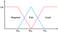 | Production decline rate (r2) | 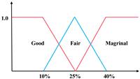 |
| Water-cut increasing rate (r3) | 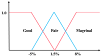 | Energy-retention degree (r4) | 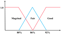 |
| Waterflooding reserves utilization degree (r5) |  | Waterflooding reserves control degree (r6) |  |
| Injectionwithdrawal ratio (r7) |  | Water storage rate (r8) |  |
| Square water–oil exchange rate (r9) |  |
| No. | Single-Index UM Matrix | No. | Single-Index UM Matrix | No. | Single-Index UM Matrix |
|---|---|---|---|---|---|
| 1 | 2 | 3 | |||
| 4 | 5 | 6 | |||
| 7 | 8 | 9 | |||
| 10 | 11 | 12 | |||
| 13 | 14 | 15 | |||
| 16 | 17 | 18 | |||
| 19 | 20 | 21 | |||
| 22 | 23 | 24 | |||
| 25 | 26 |
| r1 | r2 | r3 | r4 | r5 | r6 | r7 | r8 | r9 | R | |
|---|---|---|---|---|---|---|---|---|---|---|
| r1 | 1 | 1 | 2 | 1 | 1 | 1 | 3 | 5 | 1 | 19 |
| r2 | 1 | 1 | 1 | 0.5 | 0.5 | 1 | 2 | 3 | 0.5 | 10 |
| r3 | 0.5 | 1 | 1 | 0.5 | 0.5 | 0.5 | 1 | 2 | 0.5 | 7.5 |
| r4 | 1 | 2 | 2 | 1 | 1 | 1 | 2 | 4 | 1 | 15 |
| r5 | 1 | 2 | 2 | 1 | 1 | 1 | 2 | 3 | 0.5 | 13.5 |
| r6 | 1 | 1 | 2 | 1 | 1 | 1 | 1 | 2 | 0.5 | 11.5 |
| r7 | 0.33 | 0.5 | 1 | 0.5 | 0.5 | 1 | 1 | 2 | 0.25 | 7 |
| r8 | 0.2 | 0.33 | 0.5 | 0.25 | 0.33 | 0.5 | 0.5 | 1 | 0.25 | 3.86 |
| r9 | 1 | 2 | 2 | 1 | 2 | 2 | 4 | 4 | 1 | 17 |
| r1 | r2 | r3 | r4 | r5 | r6 | r7 | r8 | r9 | |
|---|---|---|---|---|---|---|---|---|---|
| r1 | 1.0000 | 3.3316 | 3.9793 | 2.0362 | 2.4249 | 2.943 | 4.1088 | 4.9223 | 1.5181 |
| r2 | 0.3001 | 1.0000 | 1.6477 | 0.4357 | 0.5244 | 0.7201 | 1.7772 | 2.5907 | 0.3554 |
| r3 | 0.2513 | 0.6069 | 1.0000 | 0.3398 | 0.3915 | 0.4910 | 1.1295 | 1.9430 | 0.2889 |
| r4 | 0.4911 | 2.2953 | 2.9430 | 1.0000 | 1.3886 | 1.9067 | 3.0725 | 3.886 | 0.6587 |
| r5 | 0.4124 | 1.9067 | 2.5544 | 0.7201 | 1.0000 | 1.5181 | 2.6839 | 3.4974 | 0.5244 |
| r6 | 0.3397 | 1.3886 | 2.0363 | 0.5245 | 0.6587 | 1.0000 | 2.1658 | 2.9793 | 0.4124 |
| r7 | 0.2434 | 0.5626 | 0.8853 | 0.3254 | 0.3726 | 0.4617 | 1.0000 | 1.8134 | 0.2785 |
| r8 | 0.2031 | 0.3860 | 0.5167 | 0.2573 | 0.2859 | 0.3357 | 0.5514 | 1.0000 | 0.2271 |
| r9 | 0.6587 | 2.8134 | 3.4611 | 1.5181 | 1.9067 | 2.4249 | 3.5907 | 4.4041 | 1.0000 |
| r1 | r2 | r3 | r4 | r5 | r6 | r7 | r8 | r9 | |
|---|---|---|---|---|---|---|---|---|---|
| r1 | 0.0000 | 0.5227 | 0.5998 | 0.3088 | 0.3847 | 0.4688 | 0.6137 | 0.6922 | 0.1813 |
| r2 | −0.5227 | 0.0000 | 0.2169 | −0.3608 | −0.2803 | −0.1426 | 0.2497 | 0.4134 | −0.4493 |
| r3 | −0.5998 | −0.2169 | 0.0000 | −0.4688 | −0.4073 | −0.3089 | 0.0529 | 0.2885 | −0.5393 |
| r4 | −0.3088 | 0.3608 | 0.4688 | 0.0000 | 0.1426 | 0.2803 | 0.4875 | 0.5895 | −0.1813 |
| r5 | −0.3847 | 0.2803 | 0.4073 | −0.1426 | 0.0000 | 0.1813 | 0.4288 | 0.5437 | −0.2803 |
| r6 | −0.4689 | 0.1426 | 0.3088 | −0.2803 | −0.1813 | 0.0000 | 0.3356 | 0.4741 | −0.3847 |
| r7 | −0.6137 | −0.2498 | −0.0529 | −0.4876 | −0.4288 | −0.3356 | 0.0000 | 0.2585 | −0.5552 |
| r8 | −0.6923 | −0.4134 | −0.2868 | −0.5896 | −0.5438 | −0.4740 | −0.2585 | 0.0000 | −0.6438 |
| r9 | −0.1813 | 0.4492 | 0.5392 | 0.1813 | 0.2803 | 0.3847 | 0.5552 | 0.6439 | 0.0000 |
| r1 | r2 | r3 | r4 | r5 | r6 | r7 | r8 | r9 | |
|---|---|---|---|---|---|---|---|---|---|
| r1 | 1.0000 | 3.2840 | 4.6079 | 1.6397 | 2.0149 | 2.6614 | 2.7618 | 7.1233 | 1.2652 |
| r2 | 0.3045 | 1.0000 | 1.4031 | 0.4993 | 0.6135 | 0.8104 | 1.5017 | 2.1691 | 0.3853 |
| r3 | 0.2170 | 0.7127 | 1.0000 | 0.3558 | 0.4373 | 0.5776 | 1.0703 | 1.5459 | 0.2746 |
| r4 | 0.6099 | 2.0030 | 2.8104 | 1.0000 | 1.2289 | 1.6232 | 3.0079 | 4.3446 | 0.7717 |
| r5 | 0.4963 | 1.6299 | 2.2869 | 0.8137 | 1.0000 | 1.3209 | 2.4477 | 3.5354 | 0.6279 |
| r6 | 0.3757 | 1.2339 | 1.7314 | 0.6161 | 0.6281 | 1.0000 | 0.6660 | 2.6765 | 0.4754 |
| r7 | 0.2028 | 0.6659 | 0.9343 | 0.3325 | 0.4085 | 0.5396 | 1.0000 | 1.4444 | 0.2565 |
| r8 | 0.1404 | 0.4610 | 0.6469 | 0.2302 | 0.2829 | 0.3736 | 0.6923 | 1.0000 | 0.1776 |
| r9 | 0.7904 | 2.5956 | 3.6419 | 1.2959 | 1.5925 | 2.1035 | 3.8979 | 5.6301 | 1.0000 |
| r1 | r2 | r3 | r4 | r5 | r6 | r7 | r8 | r9 | |
|---|---|---|---|---|---|---|---|---|---|
| r1 | 0.0404 | 0.1346 | 0.1608 | 0.0823 | 0.0980 | 0.1189 | 0.1660 | 0.1989 | 0.0613 |
| r2 | 0.0334 | 0.1112 | 0.1832 | 0.0484 | 0.0583 | 0.0800 | 0.1976 | 0.2880 | 0.0395 |
| r3 | 0.0408 | 0.0986 | 0.1625 | 0.0552 | 0.0636 | 0.0798 | 0.1836 | 0.3158 | 0.0470 |
| r4 | 0.0289 | 0.1352 | 0.1733 | 0.0589 | 0.0818 | 0.1123 | 0.1809 | 0.2288 | 0.0388 |
| r5 | 0.0289 | 0.1334 | 0.1787 | 0.0504 | 0.0700 | 0.1062 | 0.1878 | 0.2447 | 0.0367 |
| r6 | 0.0306 | 0.1252 | 0.1836 | 0.0473 | 0.0594 | 0.0901 | 0.1952 | 0.2686 | 0.0372 |
| r7 | 0.0430 | 0.0993 | 0.1563 | 0.0574 | 0.0658 | 0.0815 | 0.1765 | 0.3201 | 0.0492 |
| r8 | 0.0574 | 0.1092 | 0.1461 | 0.0728 | 0.0809 | 0.0949 | 0.1559 | 0.2828 | 0.0642 |
| r9 | 0.0317 | 0.1354 | 0.1666 | 0.0731 | 0.0918 | 0.1167 | 0.1728 | 0.2120 | 0.0481 |
| Weight | r1 | r2 | r3 | r4 | r5 | r6 | r7 | r8 | r9 |
|---|---|---|---|---|---|---|---|---|---|
| Subjective weight | 0.2328 | 0.0756 | 0.0539 | 0.1514 | 0.1232 | 0.0816 | 0.0503 | 0.0349 | 0.1963 |
| Objective weight | 0.1171 | 0.1073 | 0.1084 | 0.1115 | 0.1097 | 0.1080 | 0.1090 | 0.1148 | 0.1143 |
| Comprehensive weight | 0.2427 | 0.0722 | 0.0520 | 0.1503 | 0.1203 | 0.0784 | 0.0489 | 0.0356 | 0.1996 |
| No. | Multi-Index Comprehensive UM Matrix | No. | Multi-Index Comprehensive UM Matrix |
|---|---|---|---|
| 1 | (μ1k)1×3 = [0.8597, 0.0914, 0.0489] | 14 | (μ14k)1×3 = [0.6069, 0.1213, 0.2718] |
| 2 | (μ2k)1×3 = [0.6575, 0.1614, 0.1811] | 15 | (μ15k)1×3 = [0.3095, 0.3297, 0.3118] |
| 3 | (μ3k)1×3 = [0.3140, 0.4482, 0.2378] | 16 | (μ16k)1×3 = [0.4679, 0.3892, 0.1429] |
| 4 | (μ4k)1×3 = [0.7202, 0.0802, 0.1996] | 17 | (μ17k)1×3 = [0.4800, 01994, 0.1216] |
| 5 | (μ5k)1×3 = [0.5555, 0.0859, 0.3586] | 18 | (μ18k)1×3 = [0.5450, 0.1678, 0.2872] |
| 6 | (μ6k)1×3 = [0.4979, 0.2382, 0.2637] | 19 | (μ19k)1×3 = [0.3858, 0.2012, 0.4130] |
| 7 | (μ7k)1×3 = [0.4671, 0.0577, 0.4752] | 20 | (μ20k)1×3 = [0.6423, 0.1096, 0.2481] |
| 8 | (μ8k)1×3 = [0.4124, 0.2056, 0.3820] | 21 | (μ21k)1×3 = [0.3601, 0.0766, 0.5634] |
| 9 | (μ9k)1×3 = [0.6505, 0.1080, 0.2485] | 22 | (μ22k)1×3 = [0.2007, 0.1514, 0.7199] |
| 10 | (μ10k)1×3 = [0.5661, 0.0651, 0.3688] | 23 | (μ23k)1×3 = [0.4443, 0.2535, 0.3022] |
| 11 | (μ11k)1×3 = [0.6001, 0.3211, 0.0788] | 24 | (μ24k)1×3 = [0.1947, 0.1154, 0.6899] |
| 12 | (μ12k)1×3 = [0.4741, 0.0166, 0.5093] | 25 | (μ25k)1×3 = [0.2586, 0.4722, 0.2812] |
| 13 | (μ13k)1×3 = [0.3548, 0.0826, 0.5626] | 26 | (μ26k)1×3 = [0.4691, 0.3531, 0.1868] |
| No. | Results from Lei [58] | Mahalanobis Distance | Minkowski Distance | Euclidean Distance |
|---|---|---|---|---|
| 1 | 89.10 | excellent | excellent | excellent |
| 2 | 81.94 | excellent | excellent | excellent |
| 3 | 79.46 | fair | fair | fair |
| 4 | 66.35 | excellent | excellent | excellent |
| 5 | 76.78 | excellent | excellent | excellent |
| 6 | 80.45 | excellent | excellent | excellent |
| 7 | 74.25 | moderate | moderate | moderate |
| 8 | 72.31 | excellent | excellent | excellent |
| 9 | 90.09 | excellent | excellent | excellent |
| 10 | 89.4 | excellent | excellent | excellent |
| 11 | 75.42 | excellent | excellent | excellent |
| 12 | 71.11 | moderate | moderate | moderate |
| 13 | 76.60 | moderate | moderate | moderate |
| 14 | 83.01 | excellent | excellent | excellent |
| 15 | 70.39 | fair | fair | fair |
| 16 | 64.17 | excellent | excellent | excellent |
| 17 | 78.29 | excellent | excellent | excellent |
| 18 | 81.22 | excellent | excellent | excellent |
| 19 | 67.35 | moderate | moderate | moderate |
| 20 | 82.79 | excellent | excellent | excellent |
| 21 | 64.31 | moderate | moderate | moderate |
| 22 | 62.97 | moderate | moderate | moderate |
| 23 | 51.30 | excellent | excellent | excellent |
| 24 | 42.23 | moderate | moderate | moderate |
| 25 | 59.37 | fair | fair | fair |
| 26 | 81.21 | excellent | excellent | excellent |
Disclaimer/Publisher’s Note: The statements, opinions and data contained in all publications are solely those of the individual author(s) and contributor(s) and not of MDPI and/or the editor(s). MDPI and/or the editor(s) disclaim responsibility for any injury to people or property resulting from any ideas, methods, instructions or products referred to in the content. |
© 2024 by the authors. Licensee MDPI, Basel, Switzerland. This article is an open access article distributed under the terms and conditions of the Creative Commons Attribution (CC BY) license (https://creativecommons.org/licenses/by/4.0/).
Share and Cite
Su, Z.; Gao, S.; Li, Z.; Li, T.; Kang, N. Integrated Waterflooding Effect Evaluation Methodology for Carbonate Fractured–Vuggy Reservoirs Based on the Unascertained Measure–Mahalanobis Distance Theory. Processes 2024, 12, 274. https://doi.org/10.3390/pr12020274
Su Z, Gao S, Li Z, Li T, Kang N. Integrated Waterflooding Effect Evaluation Methodology for Carbonate Fractured–Vuggy Reservoirs Based on the Unascertained Measure–Mahalanobis Distance Theory. Processes. 2024; 12(2):274. https://doi.org/10.3390/pr12020274
Chicago/Turabian StyleSu, Zezhong, Shihui Gao, Zhiyuan Li, Tiantai Li, and Nan Kang. 2024. "Integrated Waterflooding Effect Evaluation Methodology for Carbonate Fractured–Vuggy Reservoirs Based on the Unascertained Measure–Mahalanobis Distance Theory" Processes 12, no. 2: 274. https://doi.org/10.3390/pr12020274