Abstract
As a device for cooling charged air before it enters the cylinder, the intercooler is an indispensable part of the regular operation of a booster diesel engine. To solve the problem of the insufficient cooling performance of an intercooler for a high-power supercharged diesel engine, in this study, the flow field in the intercooler is simulated using the computational fluid dynamics (CFD) model of porous media, and the performance data measured using the steady flow test bench are used to provide boundary conditions for the calculation. The effects of the charged air mass flow rate and the tube bundle’s transverse spacing on the heat dissipation performance of the intercooler are analyzed and compared. The calculation results show that, under the condition of satisfying the regular operation of the diesel engine, the heat transfer coefficient of the intercooler heat dissipation belt increases with the increase in air mass flow and the spacing of cooling pipes, and the heat transfer coefficient can be increased by up to 57%. Still, excessive spacing of the cooling water pipes increases pressure loss in the charged air. Finally, the transverse spacing of the tube bundle is set to 17 mm, ensuring the pressure drop in the charged air, and the heat dissipation performance of the intercooler is increased by 6.04%. This paper provides a feasible solution for further optimizing the heat dissipation performance of intercoolers. Finally, grey correlation theory is used to study the correlation between air mass flow, cooling water pipe spacing, and intercooler heat dissipation performance. The correlation values are 0.8464 and 0.8497, respectively, indicating a significant relationship between air mass flow, cooling water pipe spacing, and intercooler heat dissipation performance.
1. Introduction
To meet the requirements of increasingly stringent emission regulations, the widespread use of supercharging technology in internal combustion engines has become an inevitable development trend [1,2]. However, the high-temperature and high-pressure intake air generated by a turbocharger dramatically increases the thermal and mechanical load of the internal combustion engine [3,4]. To solve the negative impact of turbocharging, engineers have developed a charge intercooler system, by placing an intercooler between the outlet of the compressor and the inlet of the engine, which could reduce the inlet temperature and increase the air density, thus improving the combustion efficiency [5,6,7]. The experiment has proven that the charge intercooling system could significantly improve engine dynamics, economy, and cleanliness without increasing the mechanical and thermal load of the engine [8]. However, at present, the intercooler applied in high-power supercharged diesel engines generally has the problem of an insufficient heat dissipation performance. It cannot meet the heat dissipation demands of the supercharged diesel engine. Therefore, optimizing the intercooler’s heat dissipation performance is necessary [9].
At present, in the process of optimizing the performance of intercoolers, the most commonly used method is the experimental method. Dong et al. [10], based on a wind tunnel experiment, studied the heat dissipation performance of a wave-fin radiator, and the numerical relationship between the airflow rate’s heat transfer performance and the pressure drop of the radiator was demonstrated. Jang et al. [11], based on an experimental analysis, analyzed the correlation between the heat exchanger’s Reynolds number, the heat transfer performance, and the air pressure drop, and their results showed that the airflow rate is directly proportional to the heat transfer and that the air pressure drop is inversely proportional to the Reynolds number. Wen [12] and Habib [13], among others, experimentally studied the influence of the flow distribution’s non-uniformity on the plate-fin intercooler’s heat dissipation performance, and, as a result, the arrangement of the cooler bundle was improved. Kays et al. [14] comprehensively studied the effects of different structural parameters on the thermal–hydraulic performance of a shutter wing using experimental methods. With the development of computer technology, computational fluid dynamics (CFD) simulation technology can be widely used in the numerical simulation of flow field states in intercoolers [15,16]. Through the analysis of the three-dimensional flow field of a model, a suitable structural optimization scheme can be found which would provide a new method for the structural optimization of intercoolers. Djemel et al. [9] used numerical simulation to study the effects of the Reynolds number and engraving shape of the internal airflow of an intercooler on the heat transfer performance of the intercooler, and they proposed a bionic model that improved thermal efficiency by 97.66% compared to the traditional simulation model. Huang et al. [17] used the multi-scale thermal analysis method to study an intercooler for automobiles. In their study, the flow field in the intercooler was analyzed using mesh refinement and data interpolation techniques; the research results provide a reference for the grid setting of the 3D model of the intercooler in this paper. Ali et al. [18] used numerical simulation to study the influence of structural parameters on thermal–hydraulic performance and proposed the flow rate and heat transfer rate correlation formula. Huminic et al. [19] used numerical methods to study the cooling effect of flat tubes, elliptical tubes, and nanofluid concentrations on gas flow. Their results show that the shape of the cooling tube has a more noticeable impact on gas flow and heat transfer than the concentration of nanofluids.
As the critical structure behind heat transfer in an intercooler, it is necessary to improve the simulation accuracy of heat dissipation fins, and a porous media model, with a high precision and small calculation requirements, is often applied to simulate the structure of such heat dissipation fins. Xin et al. [20,21] used a porous media model to simulate an aero-engine intercooler’s internal heat dissipation structure and studied the external pressure loss and heat transfer characteristics. Liu et al. [22] simulated the internal structure of an intercooler for turbocharged diesel engines using a porous media model, and the physical characteristics of the internal flow field of the integrated intercooler were studied, and the superiority of the integrated intercooler structure was verified. Masri et al. [23] simulated a plate-fin heat sink using a porous media model, predicting the temperature distribution of a full-size plate-fin heat sink.
The above-mentioned work mainly focuses on the influence of the heat dissipation fin’s structure and the airflow state in an intercooler on the heat dissipation performance of the intercooler, and there are few studies on the influence of the distribution state of the cooling water pipe and the airflow rate on the heat dissipation performance of the intercooler. Most of the current research objects are intercoolers for automobiles and aero engines, and there are few studies on intercoolers for the high-power supercharged diesel engines used in locomotives and ships.
This study aims to improve the heat dissipation performance of an intercooler for high-power supercharged diesel engines to meet the heat dissipation requirements of said engines. In this paper, the intercooler’s heat transfer and airflow state are calculated using the Ansys Fluent simulation platform. The effects of the transverse spacing of the tube bundle and the pressurized air mass flow rate on the heat dissipation performance of the intercooler were studied. A feasible scheme was provided for further optimizing the intercooler’s heat dissipation performance by analyzing internal airflow contours such as temperature, pressure, and velocity changes and the average heat transfer coefficient of the intercooler.
2. Numerical Approaches
2.1. Governing Equation
To facilitate the calculation, the following four assumptions exist in computational fluid dynamics: (1) the physical properties of fluids and solids are constants; (2) there is no slippage of the fluid on the wall; (3) the flow is constant; and (4) the effects of natural convection and radiative heat transfer are ignored [24]. The governing equation is as follows.
2.1.1. Continuity Equation
For a control element based on meshing, the continuity equation can be expressed as the amount of fluid mass flowing into the control element equal to the increase in the fluid mass in the control element within a specified calculation step [25]. Its integral form can be expressed as:
2.1.2. Equation for Conservation of Momentum
For a control element based on meshing, the acceleration law can be applied in the x, y, and z coordinate directions to obtain the momentum conservation equation; the sum of the momentum produced by all kinds of forces in the control unit is equal to the value of the increased momentum in the fluid. Its integral form can be expressed as:
2.1.3. Equation for Conservation of Energy
Following the conservation of energy principle is the most fundamental principle of all heat exchange systems [26,27]. The equation can be expressed as such that the energy added to the control element equals the net heat flowing into the control element and the sum of the work carried out by the various forces. Introducing Fourier’s law of heat conduction into the equation, we can obtain the equation for the conservation of energy related to the temperature T and the specific enthalpy h of the fluid:
where is the portion of the mechanical energy converted to heat due to viscous action, which is called the dissipation function. The calculation formula is as follows:
2.2. The Turbulence Models
In fluid mechanical turbulence, a gas’s velocity, pressure, and temperature all change randomly with time and space [28]. At present, the numerical calculation methods of turbulence can be broadly divided into the following three categories: Direct Numerical Simulation (DNS) [29,30], Large Eddy Simulation (LES), and Reynolds Average Numerical Simulation (RANS) [31]. RANS introduces solutions for various turbulence model correction parameters by assuming the time-average value of turbulence ripples. The basic idea of this method is to use the sum of the mean and the pulsation value to represent the state value of the turbulence [32], and the turbulence is regarded as the superposition of the mean and the fluctuating field. This method only needs the time-homogeneous Reynolds equation to be solved instead of the instantaneous Navier–Stokes equation [33]. It has the characteristics of high computational stability and low requirements of computer resources.
Therefore, in this paper, the standard k-ε two-equation model belonging to the Reynolds average numerical simulation method is used to numerically simulate the turbulent flow state inside the intercooler, where k is the turbulent flow energy and ε is the dissipation rate of the turbulent flow energy, and the calculation formula is as follows:
where , is an empirical constant of 0.09, is the coordinate component along the three directions of the Cartesian coordinate system, and is the velocity component along the three directions of the Cartesian coordinate system. The value of is in the range of (1, 2, 3).
In the standard model, and are the two fundamental unknowns and the corresponding transport equations are as follows:
where , , and are the empirical constants, and the model constants are = 1.43, = 1.94, and = 0.09, respectively [34].
2.3. Calculation of Heat Transfer
In the heat calculation process of the intercooler, the heat exchange between water and air in the intercooler is calculated by the following two sets of equations [35]:
3. Construction of the Experimental Platform
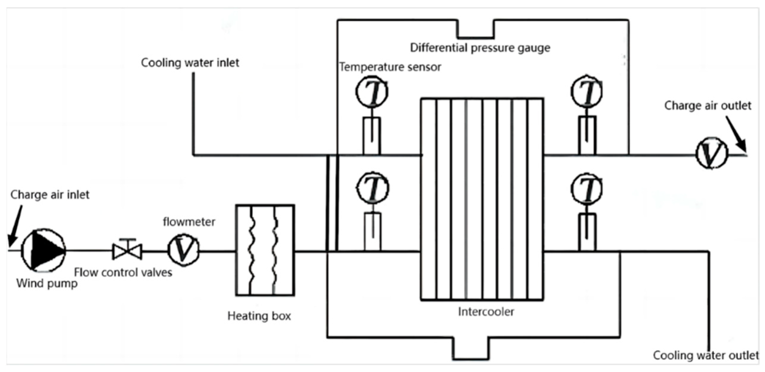
The structural principle of the steady flow test bench used in this paper is shown in Figure 1. The instruments and equipment used mainly include four thermometers (JM222 digital thermometer, resolution of 0.1 K), two flow meters (LZB series glass rotameter with a resolution of 0.001 m3/s), two U-shaped tube pressure difference gauges, one air pump, one air heating box (400 W), and a flow control valve, plus one finned tube intercooler used in this study. High-temperature charge air is generated by an air pump and air heating box, and the mass flow of air into the intercooler is precisely controlled using flow control valves and flow meters. The measurement data of the steady flow test bench are listed in Table 1. The data will be used to set the boundary conditions for the simulation model calculation and to calculate the experimental value of the heat dissipation of the intercooler.
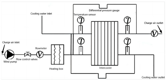
Figure 1.
Schematic diagram of the steady flow test bench.

Table 1.
Intercooled performance test results.
4. CFD Model Details
4.1. Physical Model
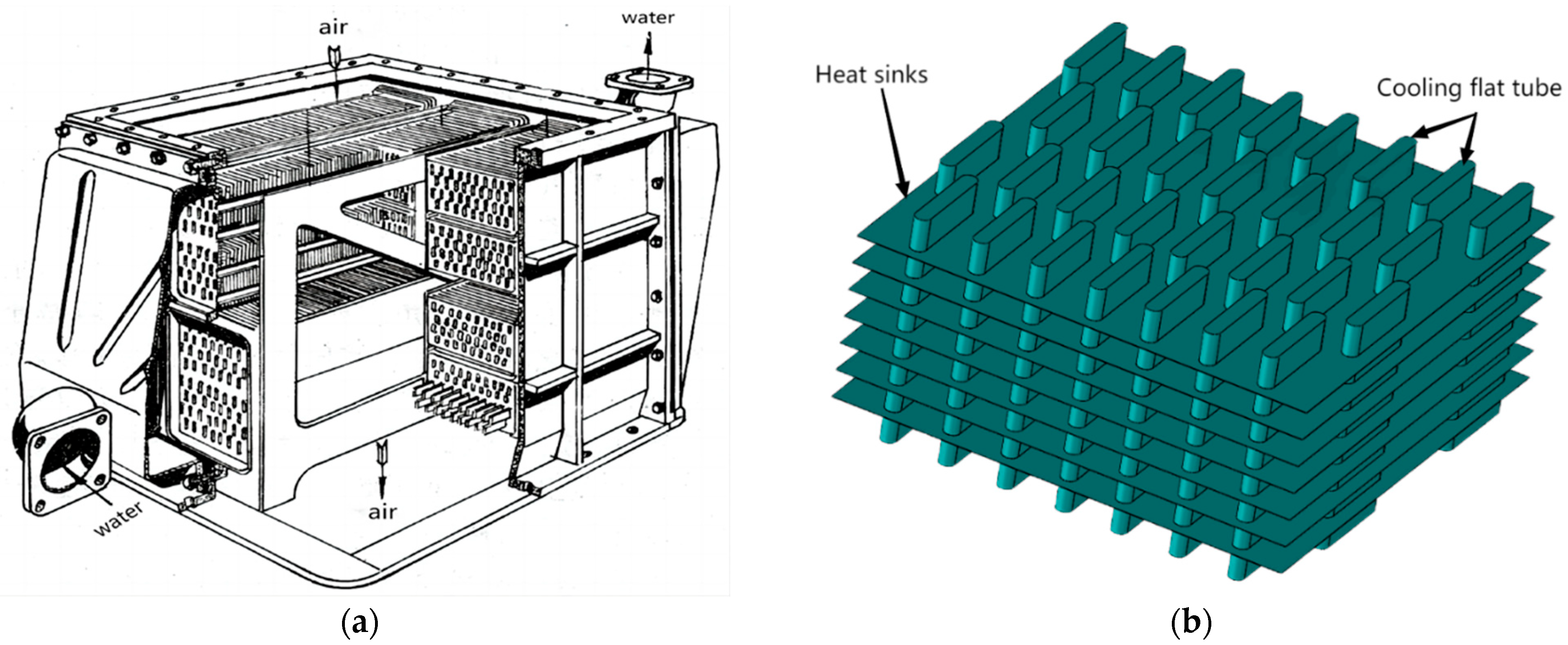
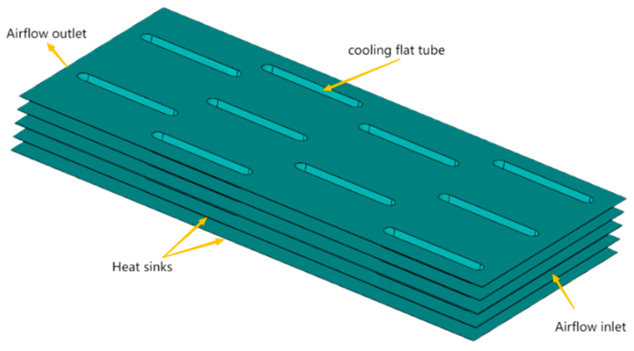
The intercooler in this study belongs to the finned tube intercooler; the cooling core is a structure with multi-layer heat sinks on the cooling flat tube, and a plurality of cooling cores are arranged in a cross manner. Then, the cooling cores are welded together by tin–lead soldering. Figure 2 is a schematic diagram of the intercooler and cooling core structure for the supercharged diesel engine, and some structural parameters are shown in Table 2.

Figure 2.
Diagram of the structure: (a) intercooler, (b) cooling core.
Table 2.
Part structural parameters of intercooler for diesel engines.
4.2. Three-Dimensional Simulation Model and Grid Settings
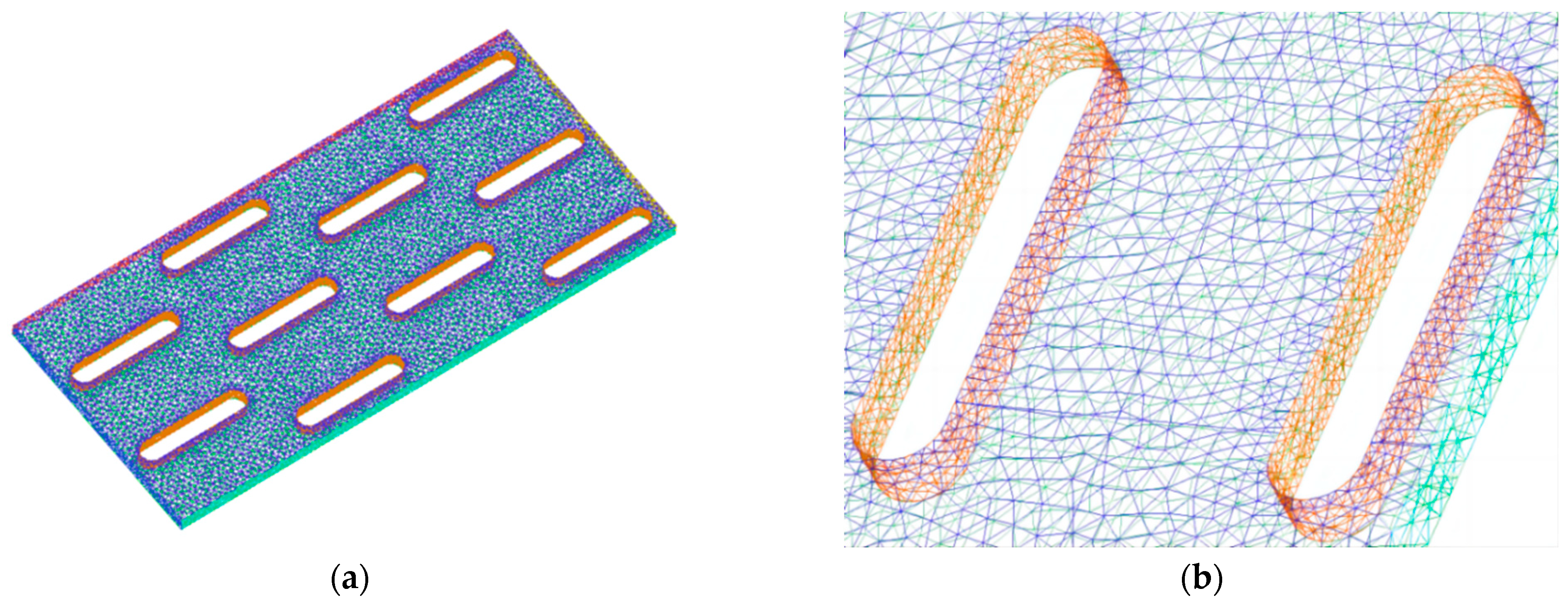
The simulation model is established according to the basic parameters of the physical model of the intercooler. To simplify the calculation, it is assumed that the airflow channels between the cooling fins are evenly distributed, the distance between the cooling water pipes is equal, and the influence of the cooling skylight of the cooling fins of the intercooler on the airflow heat transfer efficiency is ignored. Considering that the intercooler element has a large number of repetitive symmetrical structures, although the overall modeling can improve part of the calculation accuracy, it will also significantly prolong the calculation time. Therefore, in this paper, the cooling core of the middle vertical plane part is selected in the length direction of the cooling pipe for calculation and study. Figure 3 is a simplified 3D model of the intercooler. The fin material in the model is aluminum, and the thermal conductivity is 237 W·K·m−2; the heat dissipation pipe is made of copper, and the thermal conductivity is 401W·K·m−2; and the working fluids in the intercooler are air and water, and the water flow rate is 0.71 m2/s. The heat transfer coefficient of the cooling water was set at 0.52 W·K·m−2, and the heat transfer coefficient of the air was set to 0.0244 W·K·m−2, ignoring changes in the heat transfer coefficients of water and air.

Figure 3.
Simplified 3D model of the intercooler.
Setting the calculation grid is one of the most critical tasks in numerical calculation, and it critically impacts the accuracy of numerical calculation. The intercooler mainly exchanges heat with the pressurized air in the wall area of the cooling water pipe. The mechanical characteristics of the airflow in this area change more drastically. The finite volume method of the block-structured mesh is used to set the calculation grid, and the calculation model is divided into two modules: the wall area of the cooling water pipe and the other area. A common edge joins two modules. A smaller mesh size is used to divide the wall area of the cooling water pipe in detail to improve the mesh quality of the module. The other regions are meshed with a uniform mesh size, and a tetrahedral mesh is used to set up the calculation mesh of the cooler’s 3D model. The total number of computing grids is 186,681, and the total number of computing nodes is 32,243. The 3D model after setting up the calculation mesh is shown in Figure 4a, locally enlarged view of the cooling water pipe area is shown in Figure 4b.

Figure 4.
(a) Three-dimensional model after setting up the calculation mesh; (b) locally enlarged view of the cooling water pipe area.
4.3. Boundary Conditions
To solve the governing equations of the flow field in the calculation model, the boundary conditions of the governing equations must be set, and the boundary conditions of the governing equations are set as follows:
- Inlet boundary condition: the charge air inlet in the intercooler is set to the velocity boundary condition, which means that air velocity is specified.
- Outlet boundary condition: the charge air outlet in the intercooler is set to the pressure outlet boundary condition, which means that pressure and backflow are defined.
- Handling of cooling fins: to reduce the amount of computation, the cooling fins were simulated using a porous media model. The porosity of the porous region is set to be 0.9, and the viscous resistance coefficient and inertial resistance coefficient of the porous media model are calculated by the following equation:where and are the viscous resistance coefficients and inertial resistance coefficients of the porous media model, respectively [36].
The average thermal conductivity of the heat dissipation fin can be equivalent to the effective thermal conductivity of the porous media model, which is calculated as follows:
where is the porosity of the porous medium, is the heat transfer coefficient of the fluid medium in the intercooler, and is the heat transfer coefficient of the solid medium in the intercooler [37,38].
The boundary conditions of the intercooler simulation model will be set according to the intercooler performance test results in Table 1 to ensure the simulation model’s reliability and calculation accuracy.
4.4. Reliability Verification of Simulation Models
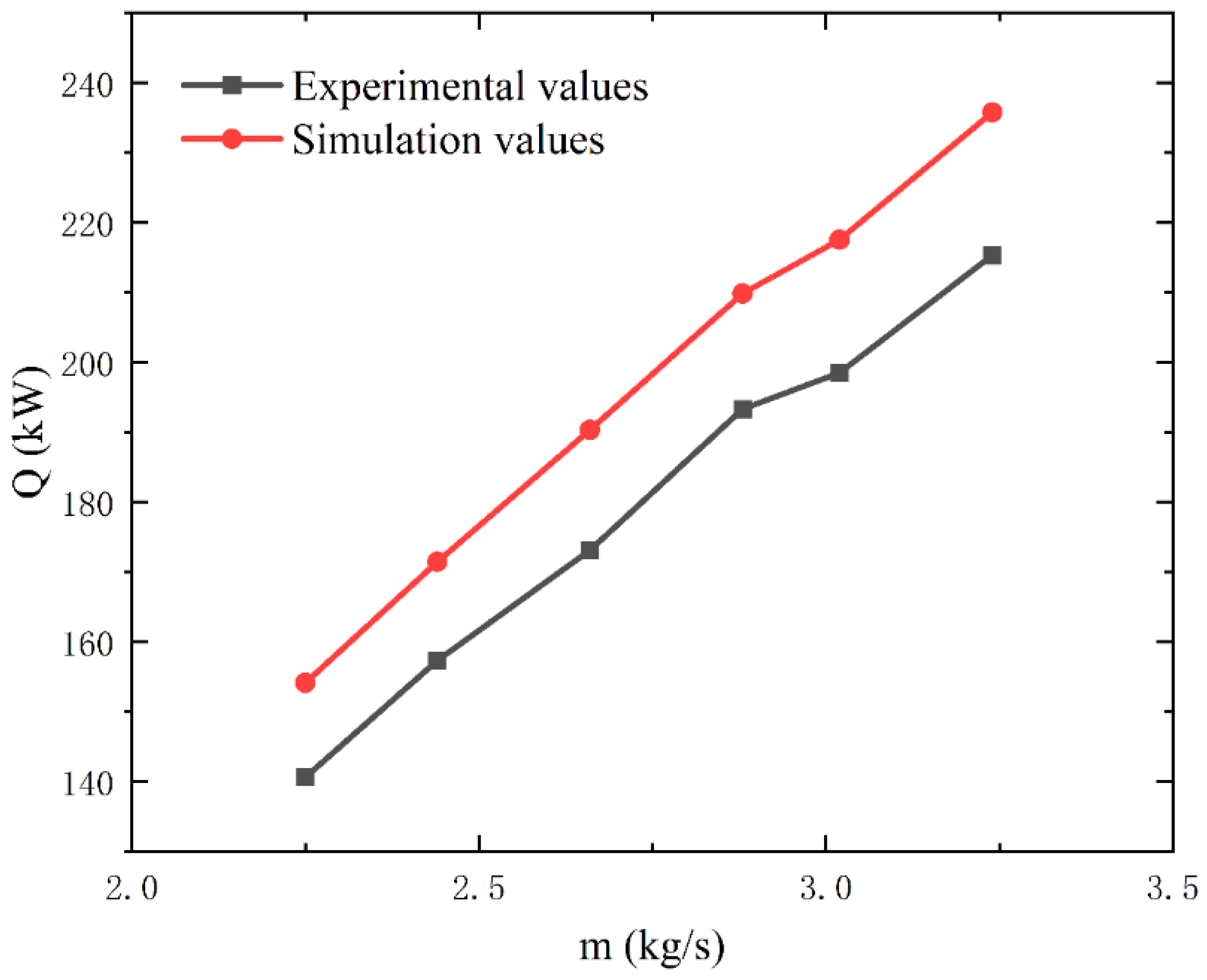
The experimental calculated value of the heat dissipation rate of the intercooler is obtained by using the relevant data measured using the steady flow test bench built in Figure 1 and combined with the calculation Formula (13) of the heat dissipation rate of the intercooler. The simulation results of the heat dissipation rate of the intercooler are compared with the experimental results, as shown in Figure 5, and the results of Figure 5 show that the heat dissipation of the intercooler calculated by simulation is higher than that of the experimental measurement, because in this study only the cooling core of the middle vertical part in the direction of the length of the cooling water pipe of the intercooler is simulated, and it is assumed that the heat dissipation rate of each part of the cooling core along the length of the cooling water pipe in the intercooler is equal. The simulation calculation results in the heat dissipation rate value of the cooling core of the selected section divided by the ratio of that part to the overall cooling core. Under experimental conditions, the heat dissipation rate of the cooling core of each part along the length of the cooling water pipe in the intercooler is not uniformly distributed. The heat dissipation rate of the cooling core close to the intercooler box is significantly lower than that of the cooling core in the middle part. Hence, the heat dissipation rate measured by the experiment is smaller than the heat dissipation rate calculated by simulation, but the changing trend of the two is the same. The maximum error between the simulated and experimental values is 9.93%. The minimum error is 8.54%, which is within the acceptable range, and the model can be used for further research.
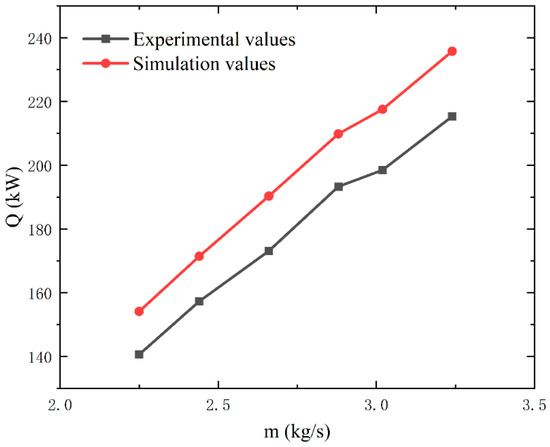
Figure 5.
Comparison of experimental and simulation data.
5. Results and Discussion
5.1. Effect of Charged Air Mass Flow on the Flow Field in the Intercooler
This study numerically simulated the intercooler’s flow and heat transfer performance under different charge air mass flows. Considering the normal working range of the supercharged diesel engine and the relevant engineering experience, the optimization scheme of the charged air mass flow of the intercooler was set to 2.25 kg/s, 2.44 kg/s, 2.66 kg/s, and other values, and the details of the flow field in the intercooler are as follows.
Figure 6 shows the temperature distribution of hot air in the intercooler as it flows through the radiator ducts; the heat is exchanged between the high-temperature air and the cooling water through the tube walls. As expected, the temperature on the air side of the intercooler shows a precise gradient distribution along the airflow direction: the maximum temperature is achieved at the inlet, and the charged air temperature gradually decreases through the layer-by-layer cooling of the cooling water pipe. The cooling effect of the intercooler on the charged air is the best in the area of the second layer of cooling water pipes; because the cooling water pipes are staggered, the area of the flow channel area of the charged air changes sharply when it flows into the channel between the second layer of cooling pipes and a large number of vortices are generated at the apex of the second layer of cooling water pipes. The convection heat exchange between the air and the water pipe in this area increases, so the charged air temperature is rapidly reduced. Hence, the cooling effect of the intercooler in this area is the most obvious. Comparing (a)–(c) in Figure 6, it can be found that the high-temperature area gradually increases with the increase in charged air mass flow. As the air mass flow increases, the newly added hot air mixes with the air that cools after heat transfer, increasing the average temperature in the heat dissipation zone area. At the same time, the increase in air mass flow will also aggravate the temperature gradient change of the charged air, which can be expressed as the drastic degree of the temperature change of the charged air per unit of time and the more severe the temperature change, the higher the convection heat transfer between the air and the water pipe in the intercooler, thus indicating that increasing the mass flow of the charged air can improve the heat transfer performance of the intercooler. This conclusion can be further demonstrated in Section 5.3.
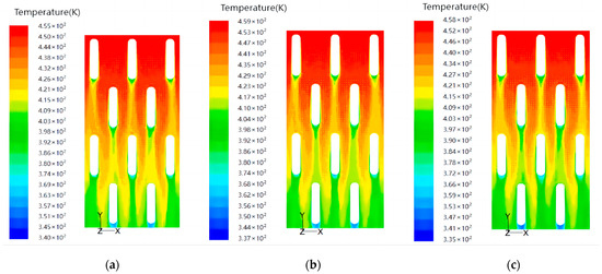
Figure 6.
Temperature contour distribution: (a) air mass flow rate 3.24 kg/s, (b) air mass flow rate 2.88 kg/s, (c) air mass flow rate 2.44 kg/s.
5.2. Effect of Tube Bundle Transverse Spacing on the Flow Field in the Intercooler
By studying the internal airflow organization of the intercooler, it was found that increasing the internal airflow disturbance of the intercooler can effectively improve the heat transfer coefficient of the intercooler and enhance its cooling effect. A large number of studies have shown that the comprehensive performance of the intercooler can be effectively improved by optimizing the spacing of the cooling pipes of the intercooler. By summarizing many previous engineering experiences, it is concluded that the best heat transfer effect will be obtained when the feasible domain of the transverse spacing of the cooling pipe of the intercooler is 14~18 mm. This paper analyses the three-dimensional flow field information in the intercooler under different cooling water pipe spacing and charged air mass flow levels to investigate the optimal transverse spacing of the cooling tube bundle in the feasible domain. In one case (air mass flow rate of 2.88 kg/s; spacing of the cooling pipes is 14, 16, and 18, respectively), the distribution characteristics of the internal pressure and velocity of the intercooler are obtained as follows.
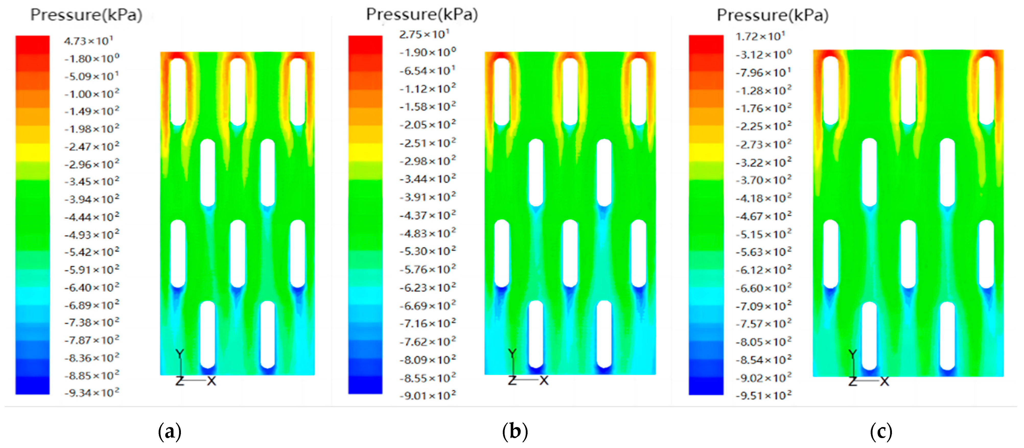
Figure 7 and Figure 8 show the pressure and velocity distribution of the air in the intercooler as it flows through the radiator duct, respectively. It can be seen that during the flow of air from the inlet to the outlet, the pressure and velocity values of the charged air flowing through the intercooler gradually decrease due to the resistance of the water pipe wall and fins, which is very similar to the changing trend of temperature. When the air comes into contact with the apex of the front arc of a water pipe, the pressure value reaches the maximum, and the velocity value is reduced to zero, forming a forward stagnation point. Then, the airflow flows around the wall of the cooling water pipe. When the airflow flows through the apex of the arc surface behind the cooling water pipe, the airflow velocity decreases to zero again due to the boundary separation effect of the airflow at that position, resulting in a rear stagnation point. There is a vortex zone behind the rear stagnation point, which reduces the cooling effect of the intercooler due to the boundary separation of the airflow flowing through this area. As the airflow flows through the passage between the cooling water pipes, the airflow rate increases, the pressure decreases, and the maximum air velocity value is obtained in this area. Due to the cross arrangement of water pipes, the air will enter the channel between the two water pipes after flowing around a certain water pipe. Hence, the flow cross-sectional area decreases, and the flow velocity increases, so the convection heat transfer between the air and the water pipe increases. Comparing the diagrams (a)–(c) in Figure 7 and Figure 8, respectively, it can be found that with the increase in the tube bundle transverse spacing, the value of pressure of the charged air at the entrance of the intercooler area selected by the simulation will gradually decrease, and the value of velocity will gradually increase. The reason is that with the increase in the transverse spacing of the cooling water pipe, the channel between the two cooling water pipes will steadily expand, and the longitudinal flow area of the airflow will increase, due to the longitudinal spacing of the cooling water pipe not changing; the change in the flow area of the airflow is more drastic when the airflow passes through the forward stagnation point, and the airflow disturbance of the charged air is increased, increasing the pressure loss of the charged air in the area. In addition, due to the squeezing effect of the change in the flow area, the flow velocity of the air when it enters the passage between the two water pipes after passing through the water pipe will be increased so that the convective heat exchange between the air and the water pipe increases. In other words, the increase in the transverse spacing of the cooling water pipes will improve the heat dissipation performance of the intercooler. This conclusion can be further demonstrated in Section 5.3.

Figure 7.
Pressure contour distribution: (a) tube bundle transverse spacing 14 mm, (b) tube bundle transverse spacing 16 mm, (c) tube bundle transverse spacing 18 mm.
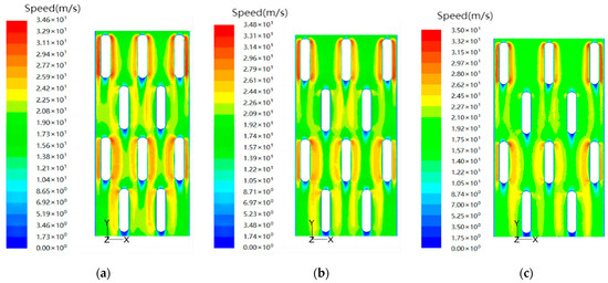
Figure 8.
Speed contour distribution: (a) tube bundle transverse spacing 14 mm, (b) tube bundle transverse spacing 16 mm, (c) tube bundle transverse spacing 18 mm.
5.3. Summary and Analysis of Results
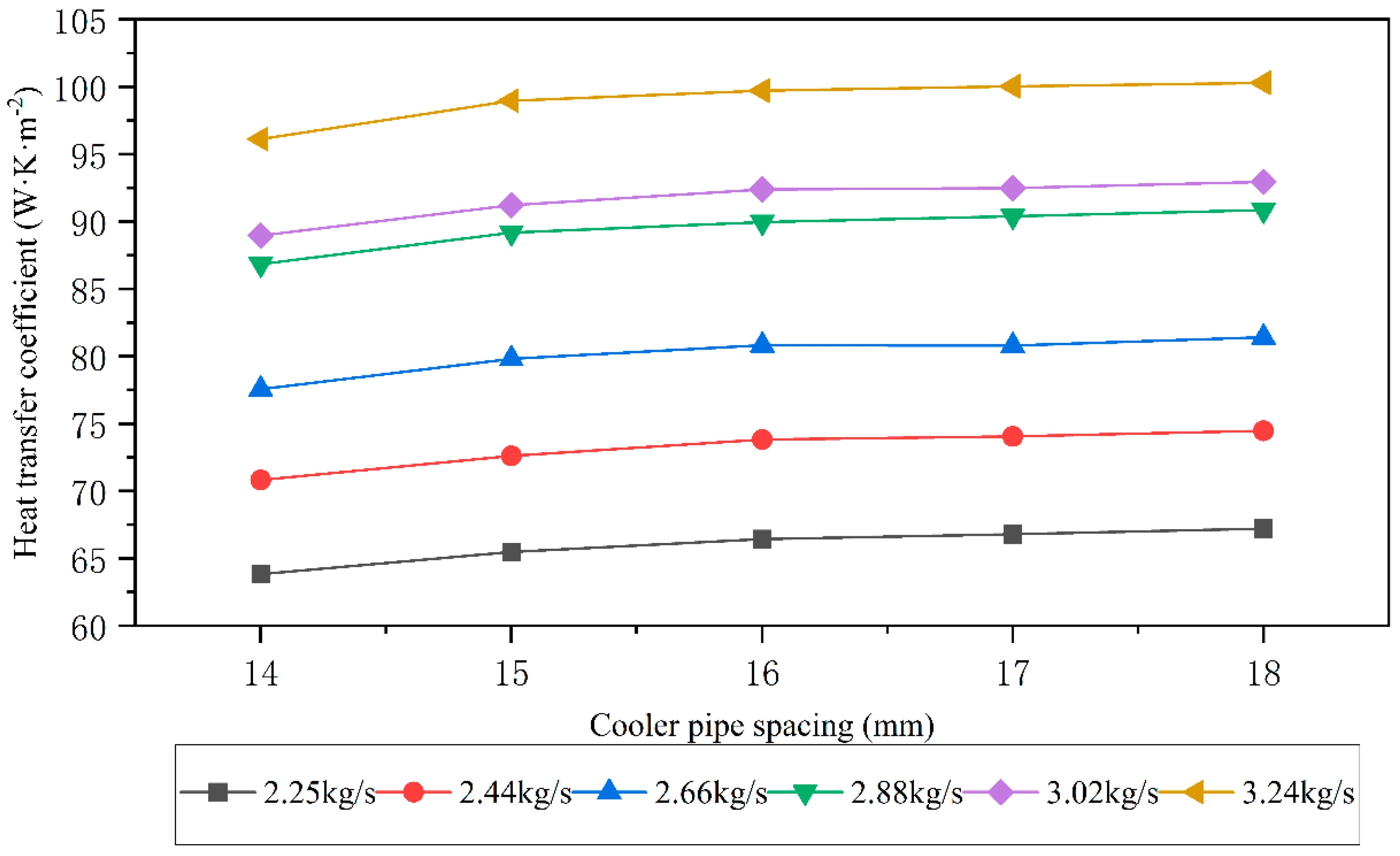
The heat transfer in the intercooler is mainly divided into the following three parts: First is the charged air and cooling water being exchanged for heat through the cooling flat tube; the second is the heat exchange between the high-temperature air and the heat dissipation belt; and last is the mixed heat exchange process between the cold and hot gases in the intercooler. In the heat transfer process of these three parts, the thermal conductivity of cooling water and high-temperature air is related to its physical properties. It has little impact on the heat transfer performance of the intercooler, so the heat dissipation performance can only be enhanced by increasing the heat transfer coefficient of the heat dissipation belt. To further study the influence of the charged air mass flow rate and tube bundle transverse spacing on the heat dissipation performance of the intercooler, the effective thermal conductivity of the porous media region is used to characterize the average heat transfer coefficient of the intercooler heat dissipation fins. Since the heat transfer process between the airflow in the intercooler and the heat dissipation band is mainly concentrated on the heat dissipation fins, the heat transfer coefficient of the heat dissipation band can be approximated by using the average heat transfer coefficient of the heat dissipation fins. The average heat transfer coefficient of the intercooler heat dissipation fins is calculated by combining the simulation data and Equation (18) to introduce different mass flow rates of charged air and change the transverse spacing of the cooling water pipes. The calculated results are shown in Figure 9.
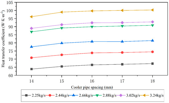
Figure 9.
The average heat transfer coefficient of the cooling fins corresponds to different cooling water pipe spacing and air mass flow rates.
As can be seen from Figure 9, under the condition of satisfying the normal operation of the supercharged diesel engine, the heat transfer coefficient of the intercooler heat dissipation belt increases with the increase in air mass flow and the spacing of cooling pipes, and the heat transfer coefficient can be increased by up to 57%. The results show that increasing the pressurized air mass flow into the intercooler and expanding the transverse spacing of the cooling pipes can effectively improve the heat dissipation performance of the intercooler. The reason why increasing the mass flow rate of charged air can improve the heat dissipation performance of the intercooler under the same cooling pipe spacing is that when the airflow rate is low, that is, the Reynolds number is small, the air flows mainly in the direction of parallel heat dissipation fins, and a boundary layer is formed at the wall surface of the heat dissipation fins, which hinders the air from contacting the heat dissipation fins. With the increase in the Reynolds number, the lateral flow of air is enhanced, the boundary layer is thinned, and the contact area between the charged air and the heat dissipation fins increases to improve the intercooler’s heat dissipation performance. As the airflow rate increases, the amount of air flowing through the channel between the two cooling pipes per unit of time increases, increasing the charged air velocity. Therefore, the heat transfer coefficient of the intercooler heat dissipation belt gradually increases.
Summarizing the above simulation data, it can be seen that expanding the tube bundle transverse spacing can effectively improve the heat dissipation performance of the intercooler within a given range of transverse spacing of the cooling water pipes. However, excessive cooling water pipe spacing will increase the pressure loss of the charged air. Since the intercooler is a crucial device for cooling the charged air, the pressure loss of the charged air should be reduced as much as possible while obtaining a sufficient cooling effect. The tube bundle transverse spacing is 17 mm.
5.4. Comparison of Optimization Results
Under the conditions of different mass flow rates of charged air, the average heat dissipation of the cooling fins obtained by the simulation calculation of the optimization scheme with a spacing of 17 mm of cooling pipes is compared with the calculated value of the average heat dissipation of the cooling fins of the original scheme, as shown in Figure 10. As can be seen from Figure 10, the heat dissipation of the improved scheme is higher than that of the original scheme under the conditions of different pressurized air mass flow, and the average heat dissipation of the two schemes increases gradually with the increase in the flow rate of the pressurized air mass, and when the mass flow rate of the charged air was 2.25 kg/s, the heat dissipation of the optimized solution increased by 6.04%. The feasibility of the structural optimization scheme is fully proven.
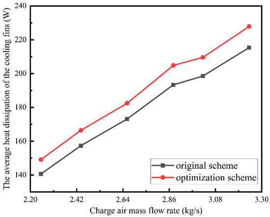
Figure 10.
Comparison of the average heat dissipation of the improved solution with the original solution.
6. Gray Correlation Analysis
Fuzzy Cluster Analysis (FCA) is a multivariate statistical analysis method. It is a commonly used method for multivariate analysis in statistics [39]. This method analyses the fuzzy correlation between multiple parameters in the multivariate problem using specific mathematical methods to objectively classify the correlation between each parameter and the principal factor. Grey correlation analysis (GRA) is a research method that determines the degree of similarity between multiple factors by comparing the degree of approximation of geometric figures, and the degree of influence of each factor can be ranked using gray correlation analysis [40]. In this paper, the grey correlation analysis method is used to study the correlation between each factor and the heat transfer coefficient of the heat dissipation band of the intercooler, and the main calculation steps are as follows.
- (1)
- Determine the calculation sequence.
The calculation sequence of the grey correlation analysis method mainly includes the reference series that reflect the characteristics of the system behavior and the comparison series that affect the behavior of the system [41]. A grey correlation calculation sequence is generally composed of a feature sequence and multiple reference sequences, which together form the calculation matrix of the grey correlation problem. By calculating the correlation of the parameters in the matrix, the correlation ranking of the parameters in the system can be displayed. The reference sequence for the grey correlation problem is as follows:
where is the reference series for computational problems, and is the data in the reference series. The above series shows the variation of the reference data.
For a system affected by m factors and n states, the combination of the data can be used to obtain a comparison matrix that affects the behavior of the system, and the result is as follows:
where is denoted as the computational problem comparison matrix, and is the data in the comparison matrix. The matrix shows the variation in the m comparison series.
In this paper, the reference sequence is expressed as the heat transfer coefficient of the heat dissipation band of the intercooler. Comparison sequences – are expressed as the mass flow of charged air, the tube bundle transverse spacing, and the pressure drop on the air side of the intercooler, respectively. The sequence matrix for each factor used for calculation in this study is as follows:
- (2)
- Normalization.
In practical problems, different data may have different properties and dimensions, and to make the original data meet the requirements of fuzzy clustering, the original data matrix needs to be normalized. It was found that the parameters selected in this paper have different physical meanings and dimensions, and to ensure calculation accuracy, they should be normalized and processed by the translation-range transformation method.
- (3)
- Calculation of grey relevance.
The grey correlation coefficient of the reference series and each comparison series is solved using the following formula. The parameterized measure of the correlation degree between the comparison and reference series can be obtained by calculating the arithmetic mean of the gray correlation coefficient at each time. The ranking of the correlation degrees of each parameter in the system can be obtained by comparing the size of the value.
where is the resolution coefficient. The value of is inversely proportional to the value of resolution, and generally is taken as a value between 0 and 1 depending on the situation. In this example, the value is 0.6.
In order to simplify the calculation process and improve the accuracy, this paper uses the 2022 version of MATLAB software for calculation. The calculation results show that the grey correlation degrees of the mass flow rate of the charged air, the transverse spacing of the cooling water pipe, and the pressure drop on the air side of the intercooler are 0.8464, 0.8497, and 0.8039, respectively. Therefore, the transverse spacing of the cooling water tube has the greatest influence on the heat transfer coefficient of the heat sink band of the intercooler, followed by the mass flow of charged air, and the pressure drop on the air side of the intercooler has the least effect. However, the gray correlation values of the above three parameters are all greater than 0.8, indicating that the three parameters have a large degree of correlation with the reference values. The heat dissipation performance of the intercooler can be improved by optimizing the above three parameter values.
7. Conclusions
In this study, the internal flow field state of an intercooler for a high-power supercharged diesel engine was numerically simulated, the performance test data of the intercooler measured by the steady flow test bench was used as the boundary condition for simulation calculation, and the heat dissipation fin structure of the intercooler was simulated by using the porous media model. The effects of the mass flow rate of the charged air and the transverse spacing of the cooling water pipes of the intercooler on the temperature, pressure, velocity flow field, and the heat transfer coefficient of the heat sink band of the intercooler were studied, and the optimal values of tube bundle transverse spacing were obtained. Finally, the grey correlation theory was used to demonstrate the grey correlation between the mass flow rate of the charged air, the tube bundle transverse spacing, and the heat transfer coefficient of the heat sink band of the intercooler, and the main conclusions are as follows.
- (1)
- Comparing the pressure and velocity flow fields of the intercooler corresponding to the transverse spacing of different cooling water pipes, it can be seen that with the increase in the spacing of the water pipes, the pressure value of the intercooler at the inlet decreases and the velocity value increases, because expanding the transverse spacing of the cooling water pipes will increase the change rate of the flow area at the inlet of the intercooler, resulting in the aggravation of the airflow disturbance of the charged air and increasing the pressure loss, and at the same time, the speed of the charged air increases due to the squeezing effect caused by the change in the area of the flow area. The increase in charged air velocity further improves the heat dissipation performance of the intercooler.
- (2)
- According to the heat transfer coefficient of the heat sink band calculated by simulation under the spacing of each cooling water pipe and the charged air mass flow, it can be seen that within the range of satisfying the regular operation of the supercharged diesel engine, the cooling pipe spacing and air mass flow are positively correlated with the heat transfer coefficient of the intercooler heat dissipation belt. That is, increasing the spacing of the cooling pipes of the intercooler and the charged air mass flow rate can improve the heat transfer capacity of the intercooler, and the heat transfer coefficient can be increased by up to 57%. However, the spacing of the cooling pipes is too high, increasing the pressure loss of the charged air. Hence, the optimal solution of the tube bundle transverse spacing is 17 mm, while ensuring the pressure drop of the charged air, and the heat dissipation of the intercooler is increased by 6.04%.
- (3)
- The grey correlation degrees of the mass flow rate of the charged air, the tube bundle transverse spacing, and the pressure drop on the air side of the intercooler relative to the heat transfer coefficient of the heat sink band of the intercooler were 0.8464, 0.8497, and 0.8039, respectively. The heat dissipation performance of the intercooler is most affected by the tube bundle transverse spacing, followed by the mass flow of the charged air, and the pressure drop on the air side of the intercooler is the least affected. The grey correlation values of the three parameters are all greater than 0.8, indicating that the three parameters have a large degree of correlation with the heat transfer capacity of the intercooler. The heat dissipation performance of the intercooler can be improved by optimizing the above three parameter values.
- (4)
- The heat dissipation rate of the intercooler obtained based on the porous media model was compared with the experimental value measured by the steady flow test bench; the data consistency was good, the error was within 10%, and the heat dissipation performance of the intercooler can be studied by using the model. The design of the intercooler structure through the simulation results can effectively reduce the R&D investment in design and reduce the R&D cost of the enterprise.
Author Contributions
Conceptualization, H.J.; software, H.J., H.W. and F.J.; formal analysis, H.J., F.J. and H.W.; investigation, H.J., H.W., F.J., J.H. and L.H.; resources, H.J.; writing—original draft preparation, H.J., H.W. and F.J.; writing—review and editing, H.J., H.W., F.J., J.H. and L.H.; supervision, H.J.; funding acquisition, H.J., F.J., L.H. and J.H. All authors have read and agreed to the published version of the manuscript.
Funding
This work is supported by the National Natural Science Foundation of China and the Guangxi University of Science and Technology Doctoral Fund Project, grant numbers NO.6196300006 and 21Z34, respectively. This study was also supported by two independent research projects from the Guangxi Key Laboratory of Automotive Parts and Vehicle Technology, with project numbers 2022GKLACVTZZ02 and 2022GKLACVTZZ03.
Data Availability Statement
All data used to support the findings of this study are included within the article.
Acknowledgments
All individuals included in this section have consented to the acknowledgement.
Conflicts of Interest
The authors declare that there are no conflicts of interest regarding the publication of this paper.
Nomenclature
| The volume of the controlling element (m3) | |
| The area of the control element (m2) | |
| The density of the fluid in the inflow control element (kg/m3) | |
| The volume force per unit mass of the control element (N) | |
| The viscous force on the surface of the control element (N) | |
| The pressure on the surface of the control element (N/m2) | |
| The thermal conductivity of the fluid | |
| The internal heat source of the fluid | |
| The work carried out by the surface force on the fluid element | |
| The production term of turbulent kinetic energy due to the mean velocity gradient | |
| Due to the buoyancy-induced turbulent kinetic energy production term | |
| The directional component of the acceleration of gravity | |
| The turbulent Prandtl number | |
| The pulsating expansion part of the compressible turbulence | |
| The turbulent Mach number | |
| The Prandtl numbers corresponding to turbulent kinetic energy | |
| The Prandtl numbers corresponding to the dissipation rate | |
| The heat transfer rate per unit of time | |
| The area of the heat dissipation area | |
| The logarithmic value of the average temperature difference | |
| The average heat transfer coefficient of the intercooler | |
| The cold fluid temperatures at the inlet of the intercooler | |
| The hot fluid temperatures at the inlet of the intercooler | |
| The cold fluid temperatures at the outlet of the intercooler | |
| The hot fluid temperatures at the outlet of the intercooler |
References
- Tang, X.; Shi, Q.; Li, Z.; Xu, S.; Li, M. Research on the influence of the guide vane on the performances of intercooler based on the end-to-end prediction model. Int. J. Heat Mass Transf. 2022, 192, 122903. [Google Scholar] [CrossRef]
- Liu, S.; Tu, A.; Li, Y.; Zhu, D. Optimization Design and Comparative Analysis of Enhanced Heat Transfer and Anti-Vibration Performance of Twisted-Elliptic-Tube Heat Exchanger: A Case Study. Energies 2023, 16, 6336. [Google Scholar] [CrossRef]
- Engkuah, S.; Nasution, H.; Abdul Aziz, A. Performance Characteristic Study on Air to Water Intercooler. Appl. Mech. Mater. 2016, 819, 42–45. [Google Scholar] [CrossRef]
- Muqeem, M. Turbocharging with Air Conditioner Assisted Intercooler. IOSR J. Mech. Civ. Eng. 2012, 2, 38–44. [Google Scholar] [CrossRef]
- Yu, Q.; Chai, H.L. The Effect of Compressible Flow on Heat Transfer Performance of Heat Exchanger by Computational Fluid Dynamics (CFD) Simulation. Entropy 2019, 21, 829. [Google Scholar] [CrossRef]
- Yaïci, W.; Ghorab, M.; Entchev, E. 3D CFD analysis of the effect of inlet air flow maldistribution on the fluid flow and heat transfer performances of plate-fin-and-tube laminar heat exchangers. Int. J. Heat Mass Transf. 2014, 74, 490–500. [Google Scholar] [CrossRef]
- Yu, C.; Zhang, W.; Xue, X.; Lou, J.; Lao, G. Analysis of Water-Cooled Intercooler Thermal Characteristics. Energies 2021, 14, 8332. [Google Scholar] [CrossRef]
- Zhang, Q.; Qin, S.; Ma, R. Simulation and experimental investigation of the wavy fin-and-tube intercooler. Case Stud. Therm. Eng. 2016, 8, 32–40. [Google Scholar] [CrossRef]
- Djemel, H.; Ben Salem, M.; Baccar, M.; Mseddi, M. Three-dimensional numerical study of the intercooler equipped with vortex generators. Heat Transf. Res. 2017, 48, 715–740. [Google Scholar] [CrossRef]
- Dong, J.Q.; Su, L. Experimental study on thermal-hydraulic performance of a wavy fin-and-flat tube aluminum heat exchanger. Appl. Therm. Eng. 2013, 51, 32–39. [Google Scholar] [CrossRef]
- Seo, J.; Cho, C.; Lee, S.; Choi, Y. Thermal Characteristics of a Primary Surface Heat Exchanger with Corrugated Channels. Entropy 2015, 18, 15. [Google Scholar] [CrossRef]
- Wen, J.; Li, Y.; Zhou, A. PIV experimental investigation of entrance configuration on flow maldistribution in plate-fin heat exchanger. Cryogenics 2006, 46, 37–48. [Google Scholar] [CrossRef]
- Habib, M.; Mansour, R.; Said, S. Evaluation of flow maldistribution in air-cooled heat exchangers. Comput. Fluids 2009, 38, 677–690. [Google Scholar] [CrossRef]
- Kays, W.; London, A. Compact Heat Exchangers; McGraw-Hill: New York, NY, USA, 1984. [Google Scholar]
- Liu, Y.; Yu, C.; Qin, S.; Wang, X.; Lou, J. Effect of transverse flow in porous medium on heat exchanger simulation optimization. Trans. Can. Soc. Mech. Eng. 2020, 44, 419–426. [Google Scholar] [CrossRef]
- Liu, Z.; Sun, M.; Huang, Y.; Li, K.; Wang, C. Investigation of heat transfer characteristics of high-altitude intercooler for piston aero-engine based on multi-scale coupling method. Int. J. Heat Mass Transf. 2020, 156, 119898. [Google Scholar] [CrossRef]
- Huang, Y.; Liu, Z.; Lu, G.; Yu, X. Multi-scale thermal analysis approach for the typical heat exchanger in automotive cooling systems. Int. Commun. Heat Mass Transf. 2014, 59, 75–87. [Google Scholar] [CrossRef]
- Sadeghianjahromi, A.; Nematih, K.S. Developed correlations for heat transfer and flow friction characteristics of louvered finned tube heat exchangers. Int. J. Therm. Sci. 2018, 129, 135–144. [Google Scholar] [CrossRef]
- Huminic, G.; Huminic, A. A numerical approach on hybrid nanofluid behavior in laminar duct flow with various cross sections. J. Therm. Anal. Calorim. 2020, 140, 2097–2110. [Google Scholar] [CrossRef]
- Zhao, X.; Grönstedt, T. Conceptual design of a two-pass cross-flow aeroengine intercooler. Proc. Inst. Mech. Eng. Part G J. Aerosp. Eng. 2014, 229, 2006–2023. [Google Scholar] [CrossRef]
- Zhao, X.; Tokarev, M.; Adi Hartono, E.; Chernoray, V.; Grönstedt, T. Experimental Validation of the Aerodynamic Characteristics of an Aero-engine Intercooler. J. Eng. Gas Turbines Power 2017, 139, 1201–1203. [Google Scholar] [CrossRef]
- Sheng, Y.; Liu, Z. Research on the integrated intercooler intake system of turbocharged diesel engine. Int. J. Automot. Technol. 2020, 21, 339–349. [Google Scholar]
- Masri, A.A.; Blum, M.L. A 3D Model for predicting the Temperature Distribution in a Full Scale APU SOFC Short Stack under Transient operating conditions. Appl. Energy 2014, 135, 539–547. [Google Scholar] [CrossRef]
- Connect, P.; Learn, S. Heat and Mass Transfer: Fundamentals and Applications. Bus. Econ. 2014, 15, 774. [Google Scholar]
- Jones, W.; Launder, B. The prediction of laminarization with a two-equation model of turbulence. Int. J. Heat Mass Transf. 1972, 15, 301–314. [Google Scholar] [CrossRef]
- Wu, J.; Tao, W. Effect of longitudinal vortex generator on heat transfer in rectangular channels. Appl. Therm. Eng. 2012, 37, 67–72. [Google Scholar] [CrossRef]
- Fluent Inc. (FLUENT, v6).3 User Manual; Fluent Inc.: New Lebanon, NH, USA, 2008. [Google Scholar]
- Yang, L.; Sicheng, Q. The optimization design of off-highway machinery radiator based on genetic algorithm and e-NTU. Acta Tech. (Former. Acta Tech. CSAV) 2017, 62, 465–476. [Google Scholar]
- Mesbah, M.; Georgievich Gribin, V.; Souri, K. Evaluation of different turbulence models in simulating the subsonic flow through a turbine blade cascade. IOP Conf. Ser. Mater. Sci. Eng. 2021, 1092, 012064. [Google Scholar] [CrossRef]
- Iyer, A.; Abe, Y.; Vermeire, B.; Bechlars, P.; Baier, R.; Jameson, A.; Witherden, F.; Vincent, P. High-Order Accurate Direct Numerical Simulation of Flow over a MTU-T161 Low Pressure Turbine Blade. Comput. Fluids 2021, 15, 104989. [Google Scholar] [CrossRef]
- Nakhchi, M.; Rahmati, M. Direct numerical simulations of flutter instabilities over a vibrating turbine blade cascade. J. Fluids Struct. 2021, 104, 103324. [Google Scholar] [CrossRef]
- Gadde, S.N.; Liu, L.; Stevens, R.J.A.M. Effect of low-level jet on turbine aerodynamic blade loading using large-eddy simulations. J. Phys. Conf. Ser. 2021, 1934, 012001. [Google Scholar] [CrossRef]
- Yu, C.; Xue, X.; Shi, K.; Shao, M.; Liu, Y. Comparative Study on CFD Turbulence Models for the Flow Field in Air Cooled Radiator. Processes 2020, 8, 1687. [Google Scholar] [CrossRef]
- Taira, K.; Brunton, S.; Dawson, S.; Rowley, C.; Colonius, T.; McKeon, B.; Ukeiley, L. Modal analysis of fluid flows: An overview. AIAA J. 2017, 55, 4013–4041. [Google Scholar] [CrossRef]
- Launder, J.; Dong, B. Spalding, Mathematical Models of Turbulence; Academic Press: London, UK, 1972. [Google Scholar]
- Fakheri, A. The Shell and Tube Heat Exchanger Efficiency and Its Relation to Effectiveness. In Proceedings of the ASME 2003 International Mechanical Engineering Congress and Exposition, Washington, DC, USA, 15–21 November 2003. ASME Paper IMECE2003-41633. [Google Scholar]
- Fluent Inc. User’s Guide, 7.19.6. FLUENT 6.2 Documentation; Fluent Inc.: New York, NY, USA, 2005. [Google Scholar]
- Dong, J.; Chen, J.; Chen, Z.; Zhou, Y.; Zhang, W. Heat transfer and pressure drop correlations for the wavy fin and flat tube heat exchangers. Appl. Therm. Eng. 2007, 27, 2066–2073. [Google Scholar]
- Zhang, X.; Jin, F.; Liu, P. A grey relational projection method for multi-attribute decision making based on intuitionistic trapezoidal fuzzy number. Appl. Math. Model. 2013, 37, 3467–3477. [Google Scholar] [CrossRef]
- Zhang, Z.; Li, J.; Tian, J.; Xie, G.; Tan, D.; Qin, B.; Huang, Y.; Cui, S. Effects of Different Diesel-Ethanol Dual Fuel Ratio on Performance and Emission Characteristics of Diesel Engine. Processes 2021, 9, 1135. [Google Scholar] [CrossRef]
- Li, M.; Li, Y.; Jiang, F.; Hu, J. An Optimization of a Turbocharger Blade Based on Fluid–Structure Interaction. Processes 2022, 10, 1569. [Google Scholar] [CrossRef]


Disclaimer/Publisher’s Note: The statements, opinions and data contained in all publications are solely those of the individual author(s) and contributor(s) and not of MDPI and/or the editor(s). MDPI and/or the editor(s) disclaim responsibility for any injury to people or property resulting from any ideas, methods, instructions or products referred to in the content. |
© 2024 by the authors. Licensee MDPI, Basel, Switzerland. This article is an open access article distributed under the terms and conditions of the Creative Commons Attribution (CC BY) license (https://creativecommons.org/licenses/by/4.0/).